Abstract
The Harris Hawks Optimization algorithm (HHO) is a sophisticated metaheuristic technique that draws inspiration from the hunting process of Harris hawks, which has gained attention in recent years. However, despite its promising features, the algorithm exhibits certain limitations, including the tendency to converge to local optima and a relatively slow convergence speed. In this paper, we propose the multi-strategy improved HHO algorithm (MSI-HHO) as an enhancement to the standard HHO algorithm, which adopts three strategies to improve its performance, namely, inverted S-shaped escape energy, a stochastic learning mechanism based on Gaussian mutation, and refracted opposition-based learning. At the same time, we conduct a comprehensive comparison between our proposed MSI-HHO algorithm with the standard HHO algorithm and five other well-known metaheuristic optimization algorithms. Extensive simulation experiments are conducted on both the 23 classical benchmark functions and the IEEE CEC 2020 benchmark functions. Then, the results of the non-parametric tests indicate that the MSI-HHO algorithm outperforms six other comparative algorithms at a significance level of 0.05 or greater. Additionally, the visualization analysis demonstrates the superior convergence speed and accuracy of the MSI-HHO algorithm, providing evidence of its robust performance.
Keywords:
optimization; global optimization; metaheuristic algorithm; Harris hawks optimization; MSI-HHO MSC:
49M37; 68T20
1. Introduction
Optimization is a crucial process involved in identifying the most favorable value among all feasible options for a particular problem. In the domain of traditional optimization methods, it is imperative to establish a precise mathematical model of the problem; determine its constraints, objective function, and decision variables; and subsequently leverage the gradient information of the objective function to effectively solve the problem.
However, the practical engineering optimization problems have become increasingly complicated, exhibiting characteristics such as multiple variables, objectives, constraints, extremes, as well as non-linearity and non-analyticity, which are commonly referred to as NP-hard problems in mathematics [1]. Establishing mathematical models for these problems is often challenging due to the discontinuous and non-differentiable objective functions, as well as the high dimensionality of variables. Consequently, traditional optimization methods are inadequate for solving such problems [2].
In recent years, metaheuristic optimization algorithms have gained prominence due to their advantages of not relying on mathematical models or the gradient information of the objective functions. Furthermore, they exhibit the ability to identify satisfactory solutions and have a low dependence on specific optimization problems. As a result, they have been widely applied in engineering fields such as artificial intelligence, robotics, system control, data analysis, and image processing, playing an increasingly vital role [3].
Two different criteria are widely used to categorize metaheuristic algorithms according to the current literature. The first criterion refers to the number of agents searching within the algorithm, while the second criterion pertains to the underlying sources of inspiration employed to develop the algorithm [4].
Based on the number of agents, metaheuristic algorithms can be further classified into two categories, i.e., the Trajectory-based and Population-based algorithms. The former usually begin with a randomly generated solution and progressively refine it over iterations. Examples of such algorithms include Simulated Annealing (SA) [5], Iterated Local Search (ILS), etc. Actually, a considerable number of prominent metaheuristic algorithms belong to the category of Population-based algorithms, e.g., Particle Swarm Optimization (PSO) [6], Genetic Algorithm (GA) [7], Grey Wolf Optimizer (GWO) [8], and so on. These algorithms start with a randomly generated population of solutions and iteratively improve them. Population-based algorithms offer distinctive advantages of effectively exploring the search space, sharing information among individuals, and increasing the likelihood of finding the global optimal solution.
According to the second criterion, we divide metaheuristic algorithms into four primary categories based on their sources of inspiration, i.e., evolutionary phenomena, physical rules, human-related concepts, and the swarm intelligence of creatures. Algorithms based on evolutionary phenomena can be mainly categorized into four branches, including the extensively employed GA [7] and Differential Evolution (DE) [9], as well as the Evolution Strategies (ES) [10] and Evolution Programming (EP) [11]. Physics-based algorithms comprise renowned techniques like SA [5], Gravitational Search Algorithm (GSA) [12], and the state-of-the-art Artificial Electric Field Algorithm (AEFA) [13], which has been proposed in recent years, among others. Algorithms based on human-related concepts include Harmony Search (HS) [14], Teaching–learning-based Optimization (TLBO) [15], Student Psychology-Based Optimization (SPBO) [16], etc. The final category encompasses algorithms inspired by the swarm intelligence observed in creatures, constituting the largest and most extensively utilized branch. Representative algorithms within this domain include PSO [6], GWO [8], Seagull Optimization Algorithm (SOA) [17], Whale Optimization Algorithm (WOA) [18], and Artificial Bee Colony (ABC) [19], among others.
The HHO algorithm is an advanced metaheuristic optimization algorithm based on the swarm intelligence of creatures, which draws inspiration from the prey hunting behavior of Harris hawks [20]. The HHO algorithm comprises two distinct stages, i.e., the exploration phase and the exploitation phase, which correspond to global exploration and local exploitation of the search space, respectively. The random component of prey escape energy facilitates the seamless transition between the exploration and exploitation phases, ensuring a balanced relationship between them. Additionally, the Lévy flight is utilized in the exploitation phase to help agents escape from local optimal solutions, enhancing the global search capability of the algorithm. HHO offers several advantages such as few control parameters, high search efficiency and accuracy, and so on [21]. It has found widespread applications in various fields, including neural networks [22], image segmentation [23], parameter identification of photovoltaic cells and modules [24], satellite image denoising [25], and others.
However, the HHO algorithm still exhibits certain limitations, such as a tendency to converge towards local optima [21] and a relatively slow convergence speed [26]. Aiming at addressing these shortcomings, we propose a novel multi-strategy improved HHO algorithm, named MSI-HHO. Firstly, an inverted S-shaped function is utilized to characterize the dynamics of prey escape energy, achieving a better balance between exploration and exploitation. Secondly, a stochastic learning mechanism based on Gaussian mutation is incorporated to enhance the search accuracy of the algorithm. Additionally, the refracted opposition-based learning technique is employed to assist the agents in escaping from local optimal solutions, thereby improving the global search capacity of the algorithm. Subsequently, we conduct comprehensive experiments of the proposed MSI-HHO on 23 classical benchmark functions and CEC 2020 benchmark functions. The assessment outcomes are analyzed using two non-parametric test methods, i.e., the Wilcoxon test and Friedman test, as well as the visualization method, i.e., convergence graphs. Remarkably, the results clearly demonstrated the superior performance of MSI-HHO over both the standard HHO and other algorithms used for comparison.
The subsequent sections of this paper are structured as follows: Section 2 offers a comprehensive review of the standard HHO algorithm. Section 3 provides a detailed exposition of the proposed MSI-HHO as well as the three enhancement strategies. In Section 4, we elaborate on the simulation experiments, along with the corresponding test results. Finally, Section 5 presents the conclusions drawn from our study.
2. Harris Hawks Optimization
The escape energy of prey determines whether a hawk is in the exploration or exploitation phase in the HHO algorithm. Distinct search strategies are associated with different values of escape energy. Consequently, it is imperative to calculate the prey’s escape energy prior to updating the population in each iteration and subsequently determine the appropriate next stage to pursue. The escape energy of prey is mathematically defined as follows [20].
where represents the initial escape energy of the prey, which is a random number between and 1. represents the current number of iterations, and represents the maximum number of iterations.
2.1. Exploration Phase
If the escape energy of prey , it is considered that the prey is currently energetic, and the distance between the hawk and the prey remains significant. Under these circumstances, the hawk becomes less purposeful and starts searching for the prey across a large area. Two distinct strategies are employed by the hawk to update its position, depending on whether it has successfully determined the location of the prey. The HHO algorithm generates a random number, denoted as , to determine which strategy to use as below [20].
where are random numbers between 0 and 1. and represent the current and the next position of the hawk, respectively. represents the position of a hawk which is randomly chosen from the current population. is the current position of the prey, i.e., the globally fittest solution. are the upper and lower bounds of this dimension, respectively. is the current average position of the population, which is defined as below [20].
where represents the number of the population. represents the current position of the -th hawk.
2.2. Exploitation Phase
If the escape energy of prey , the algorithm transitions into the exploitation phase. During this stage, the hawk endeavors to encircle the prey. However, the prey often manages to evade the hawk due to its residual energy and deceptive maneuvers. In response to this scenario, the hawk has evolved four distinct strategies, i.e., soft besiege, hard besiege, soft besiege with progressive rapid dives, and hard besiege with progressive rapid dives. The selection of the optimal strategy for a successful hunt depends on the prey’s available energy and the effectiveness of its escape attempts. The HHO algorithm utilizes a random number, denoted as , to simulate the prey’s likelihood of escaping capture. If , it indicates that the prey has failed to escape. Conversely, if , the prey successfully evades capture. Simultaneously, the escape energy of the prey is employed to assess its current state of vitality. If , the prey remains energetic. On the contrary, if , the prey is deemed exhausted.
2.2.1. Soft Besiege
If and , the prey fails to escape but still remains energetic. The hawk opts to persist in hovering over the prey, thereby contributing to further energy depletion in the prey and augmenting the likelihood of a successful hunt. The position update formula, delineated as follows, incorporates these considerations [20].
where is the jump strength of the prey, employed to simulate the distance that the prey is capable of jumping. is a random number between 0 and 1.
2.2.2. Hard Besiege
If and , the prey fails to escape and becomes exhausted. At this time, the hawk launches a swift and forceful attack, employing a blitz tactic and rapidly closing in on the prey. The position update formula is presented as follows [20].
2.2.3. Soft Besiege with Progressive Rapid Dives
If and , the prey successfully escapes from capture and remains energetic. Under these circumstances, the hawks make a series of rapid group dives around the prey, adjusting their position and orientation based on the path taken by the prey during its escape for the subsequent attack. The position update formula is depicted below [20].
The variable represents the newly obtained position derived from the given equation above. Then, the fitness values associated with the new position and the previous position are compared to assess the efficacy of the strategy employed by the hawks. If , it indicates the successful implementation of the strategy, and the previous position will be replaced with the new position . Otherwise, the strategy fails, prompting the hawks to initiate a rapid and irregular dive to attain a new position, denoted as , which is calculated as below [20].
where is a -dimensional vector, and each component of is a uniform random number generated within the range of 0 to 1. , called the Lévy flight, is also a -dimensional vector, whose components can be obtained using the following procedure [20].
where variables and are random numbers uniformly distributed between 0 and 1. The variable represents a constant value, which is typically set to 1.5 as a default.
Based on the previous discussion, the strategy of soft besiege with progressive rapid dives can be summarized as follows [20].
where and are given by Equation (6) and Equation (7), respectively.
2.2.4. Hard Besiege with Progressive Rapid Dives
If and , it indicates that the prey has managed to escape, albeit with a significant depletion of its escape energy. In this scenario, the hawk initiates a gradual dive, but with the primary objective of approaching the prey as closely as possible. The position update formula is as follows [20].
where is the newly obtained position. Similar to the strategy of soft besiege with progressive rapid dives, if , the previous position will be replaced with the new position . Otherwise, a new position will be assigned according to Equation (7), and will be determined based on Equation (9).
3. The Proposed Algorithm
3.1. Inverted S-Shaped Escape Energy
The search phase of the hawks is determined by the escape energy of the prey in the HHO algorithm. Typically, when the absolute value of the escape energy, denoted as , is large, the hawks are more inclined to enter the exploration phase. Conversely, they are also more likely to enter the exploitation phase. However, the escape energy of the prey exhibits a linearly decreasing trend, indicating a constant rate of energy depletion. Consequently, the rapid decline in escape energy during the early exploration phase results in a loss of population diversity and premature convergence in the subsequent exploitation phase.
In this case, we utilize an inverted S-shaped function to characterize the dynamics of the prey escape energy, which capitalizes on the characteristics of slower decline rates in the early and late stages and a faster decline rate in the middle stage. The formula defining the inverted S-shaped escape energy is presented below.
where are the parameters that control the shape of the inverted S-shaped function, which are set to 5 and , respectively. is the current number of iterations.
Figure 1 illustrates the dynamics of the proposed inverted S-shaped escape energy. As shown in Figure 1, the strategy enables the escape energy of the prey to maintain a large value for an extended period in the early stage, facilitated through the global exploration. Simultaneously, it ensures that the escape energy remains a small value for a prolonged time in the later stage, thereby promoting comprehensive local exploitation.
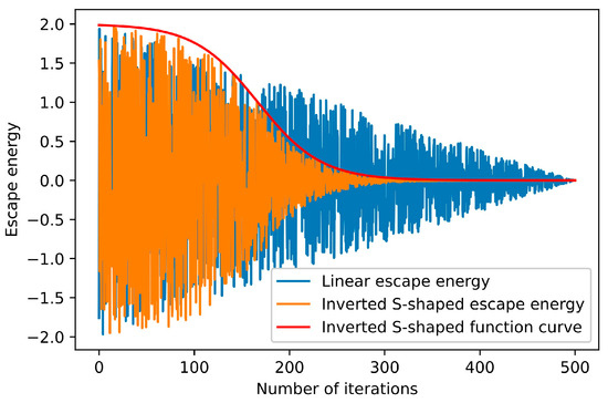
Figure 1.
The dynamics of the inverted S-shaped escape energy.
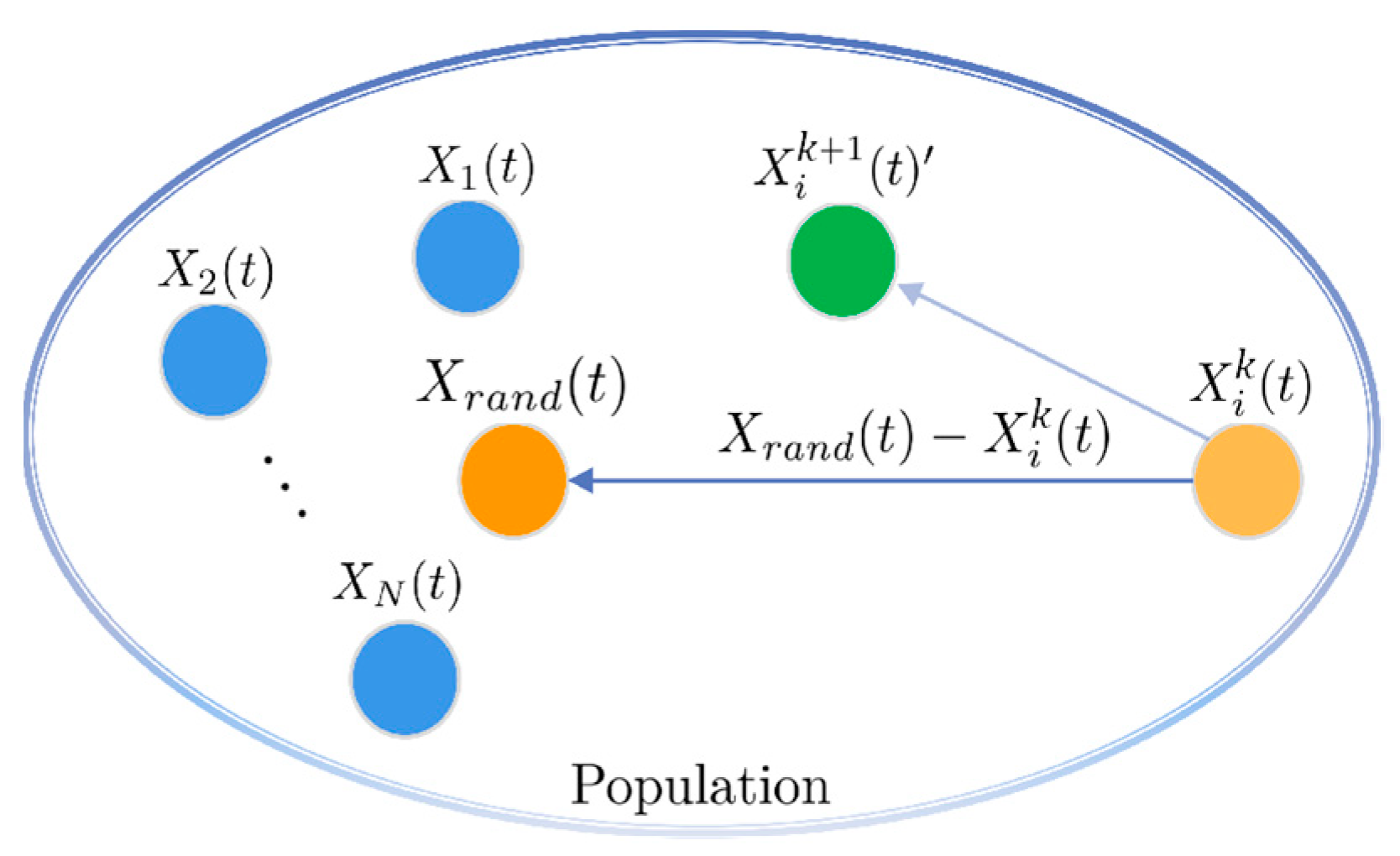
3.2. Stochastic Learning Mechanism Based on Gaussian Mutation
The HHO algorithm still faces challenges pertaining to low convergence accuracy and limited local search capabilities. In this case, we propose the stochastic learning mechanism based on Gaussian mutation to enhance the hawks’ exploitation capacities. The fundamental concept of the strategy involves applying the stochastic learning mechanism, driven by Gaussian mutation, to each hawk according to the mutation probability within each iteration. Then, a specific method, i.e., greedy selection, is utilized to determine the acceptance of the new solutions obtained. We refer to this process as “researching”. The formula of the stochastic learning mechanism based on Gaussian mutation is defined as below.
where represents the position of -th hawk after performing researchings in the -th iteration, with and . The parameter signifies the number of researchings that will be conducted. Moreover, represents the position of a hawk randomly selected from the population in the -th iteration. The term refers to a -dimensional random vector, wherein each component is a random number following a Gaussian distribution with a standard deviation of and a mean value of . Additionally, the operator ‘’, known as the Hadamard Product, signifies the element-wise multiplication of corresponding components in two vectors.
As illustrated in Figure 2, the hawk integrates the positional information of a random individual, denoted as , and the result of the Gaussian mutation to reach a new position, denoted as . Subsequently, the acceptance of this new position is determined based on the greedy selection strategy. When the objective is to minimize the optimization function, the implementation of the greedy selection strategy is as follows.

Figure 2.
The stochastic learning mechanism based on Gaussian mutation.
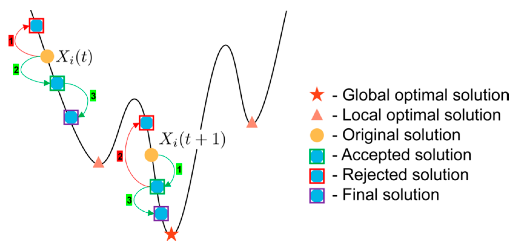
The position of the hawk will be replaced with the final result obtained by conducting researchings. For cases when , the specific process of researchings is shown in Figure 3. The arrows depict the path followed by the hawk during the researchings, with the adjacent number representing the sequential order of the researchings. Additionally, according to the greedy selection strategy, the red arrows signify the rejection of the new solution, while the green arrows indicate acceptance. Notably, the researchings enable hawks to thoroughly explore the immediate vicinity, thereby significantly enhancing the local exploitation capability of the algorithm.

Figure 3.
The specific process of the researchings.
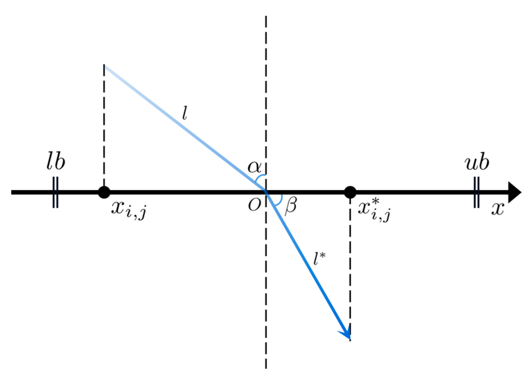
3.3. Refracted Opposition-Based Learning
Opposition-based learning (OBL) is a valuable algorithm enhancement mechanism, which extends the search space by taking the opposition solutions into account, leading to the discovery of improved solutions for the problem [27]. OBL has significantly contributed to enhancing the performance of various metaheuristic algorithms [28,29,30,31,32,33]. Building upon OBL, refracted opposition-based learning (ROBL) leverages the principles of both OBL and the refraction law of light to identify superior solutions, which has been successfully applied to improve GWO [34], WOA [35], AEFA [36], and other algorithms. We attempt to use the mechanism to improve the performance of HHO. The basic principle of ROBL is shown in Figure 4.

Figure 4.
The diagram of the refracted opposition-based learning.
In Figure 4, denotes the position of the -th individual within the population in the -th dimension. The refracted opposition solution of is represented as . The variables , , and correspond to the upper bound, lower bound, and their midpoint on this dimension, respectively. The angles and depict the angle of incidence and exit, while the lengths of the incoming and outgoing light are represented by and , respectively. Based on the definition of trigonometric functions, Equation (14) can be derived.
Based on the definition of the refractive index, i.e., , Equation (15) can be derived by combining the definition with Equation (14).
Equation (16) can be obtained by Equation (15) with making .
Referring to Equation (16), it can be observed that the opposition-based learning is actually a specific case of the refracted opposition-based learning. Specifically, when , Equation (16) reduces to the standard form of OBL as follows [27].
At the end of each iteration, the population is sorted in descending order based on their fitness values. The top individuals are selected to undergo ROBL operations, and the greedy selection strategy is employed to determine the acceptance of new solutions. Subsequently, the updated first individuals are merged with the remaining individuals to form a new population, which will be utilized in the subsequent iteration. The formula for determining is as follows.
where the operator ‘Floor’ denotes the mathematical operation of truncating the decimal portion of a numerical value, leaving only the integer part. represents the size of the population, while and denote the current and maximum iteration counts, respectively.
As evident from Equation (18), the decreases gradually from the population size to 1 as the current iteration count increases during the search process. The deliberate design enables the algorithm to explore the search space extensively during the early stages, while reducing the computation required in the later stages.
3.4. The Proposed Algorithm Combining Three Improved Strategies
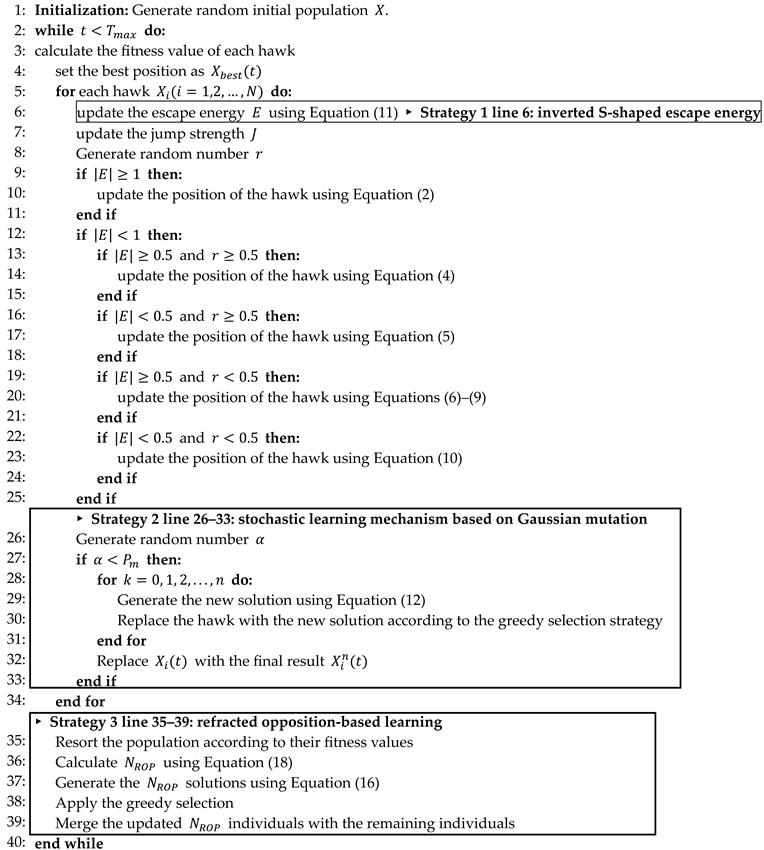
The proposed MSI-HHO algorithm is developed by integrating the above three strategies, i.e., the inverted S-shaped escape energy, the stochastic learning mechanism based on Gaussian mutation, and the refracted opposition-based learning, as well as an additional strategy called greedy selection. The specific process of the algorithm is shown in Algorithm 1.
As depicted in Algorithm 1, the three proposed improvement strategies are highlighted using bold black borderlines to indicate their respective positions and implementation processes within the MSI-HHO algorithm. Specifically, the first strategy is applied at line 6, where hawks update the escape energy of prey using the proposed Equation (11). Then, the second strategy operates on lines 26–33. After each hawk updates its position in each iteration, it continues to undergo operations defined by the second strategy, i.e., the stochastic learning mechanism based on Gaussian mutation, performing rounds of researchings. The final result is utilized for the next operations. Subsequently, the third strategy is applied at lines 35–39. Once the population completes the update for the current iteration, hawks are sorted in descending order based on their fitness values. The third strategy, i.e., the refracted opposition-based learning, is employed on the top hawks. Finally, the updated hawks are then merged with the remaining hawks, forming a new population for the next iteration. The three proposed strategies aim to improve the standard HHO algorithm from the perspectives of prey, hawks, and the population. Firstly, the inverted S-shaped escape energy strategy is introduced to optimize the utilization of limited computational resources. Secondly, the stochastic learning mechanism based on Gaussian mutation enhances the algorithm’s local exploitation capability. Lastly, the refracted opposition-based learning strategy primarily enhances the global exploration capability of the Algorithm 1.
| Algorithm 1. The multi-strategy improved HHO algorithm (MSI-HHO) | |
| Input: | Population size Maximum iterations Mutation probability Number of researchings Standard deviation and mean of Gauss distribution Refractive index |
| Output: | Global best hawk Global best fitness value |
 | |
4. Experimental Results and Discussion
To assess the efficacy of our proposed algorithm, we employ it to address the optimization problems of the 23 classical benchmark functions [12] along with the latest IEEE CEC 2020 benchmark functions [37]. These benchmark functions are elaborated in detail in Table 1 and Table 2. In Section 4.2, we conduct a comprehensive comparative analysis between our MSI-HHO algorithm and six other state-of-the-art search algorithms, namely, GSA [12], DE [9], SOA [17], WOA [18], ABC [19], and the standard HHO [20]. Furthermore, the experimental results are presented in Section 4.3, followed by non-parametric tests in Section 4.2. Section 4.4 provides graphical representations of the iterative curves for all algorithms, facilitating a more intuitive observation of their convergence.

Table 1.
The 23 classical benchmark functions.
Table 2.
The IEEE CEC 2020 benchmark functions.
All the experiments are implemented using the MATLAB 2021b development environment. The computations are performed on a 64-bit computer manufactured by Lenovo in Changsha, China, equipped with an AMD R7-4700U@2.0GH processor, 16 GB of RAM, and the Windows 10 operating system.
4.1. Benchmark Functions
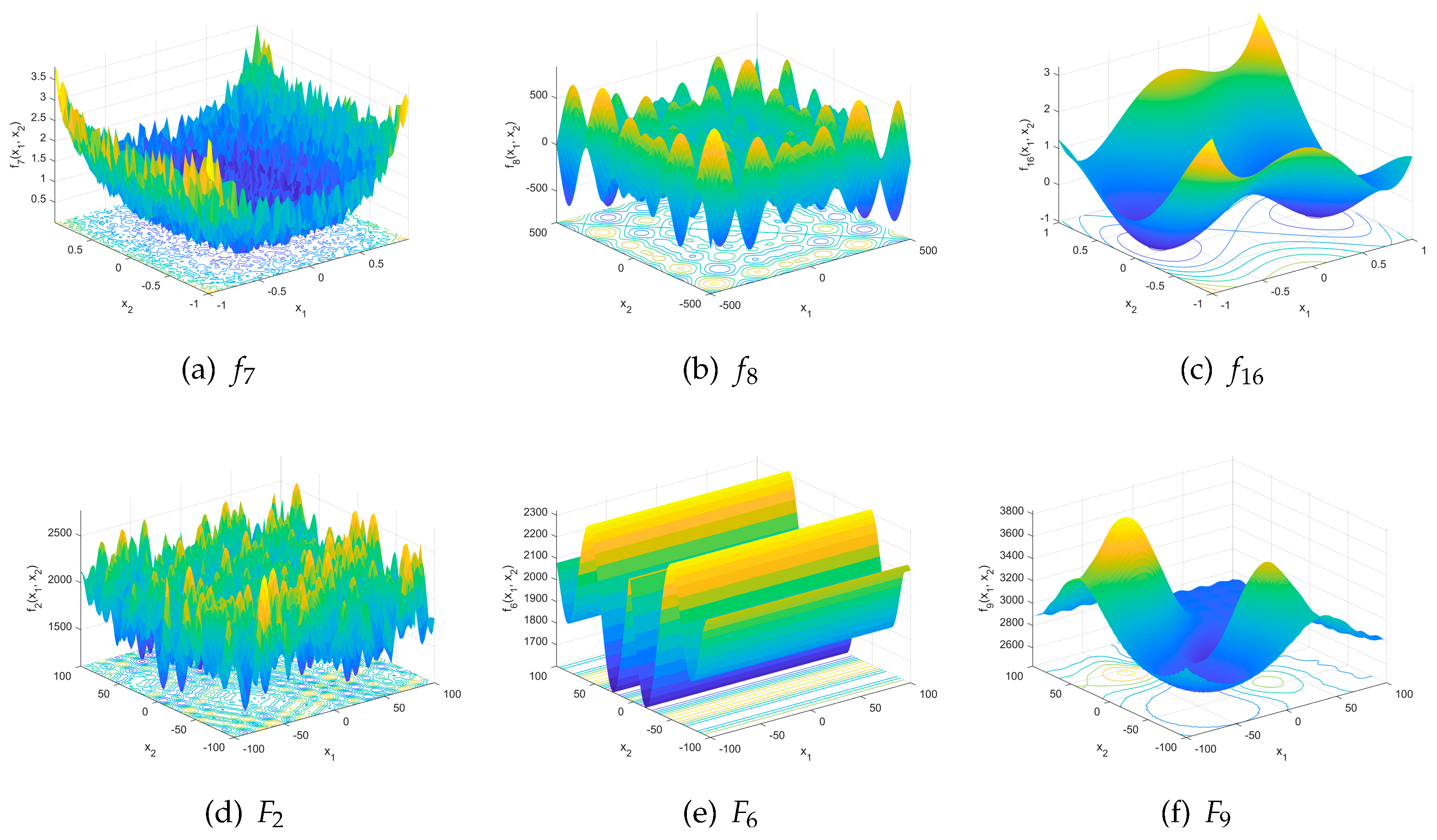
Firstly, the 23 widely used classical benchmark functions are utilized for the simulation experiments. A detailed description of these functions, including their type, definition, variable range (), dimension (), and optimal value (), is provided in Table 1. Among the functions, – represent a high-dimensional problem with . Specifically, are categorized as unimodal functions, while – are considered multimodal functions where the number of local optimal solutions increases exponentially as the problem dimension expands. The functions represent a low-dimensional problem characterized by having only a few local optimal solutions. In order to enhance the visual understanding of the characteristics of these functions, we generated three-dimensional surface graphs along with contour lines. These graphs are assigned as Figure 5a–c, representing functions , , and , respectively.
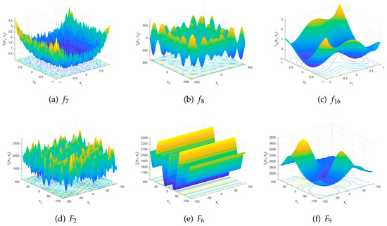
Figure 5.
The 3D surface graphs of the example test functions.
4.2. Comprehensive Comparison
The proposed MSI-HHO algorithm is compared with the standard HHO algorithm along with five other state-of-the-art algorithms, i.e., GSA, DE, SOA, WOA, and ABC. These algorithms have been extensively validated for their effectiveness and robustness in solving various engineering optimization problems. Among them, GSA is a well-known physics-based algorithm that draws inspiration from the law of universal gravitation. Furthermore, DE is also a celebrated algorithm widely recognized for its effectiveness in problem-solving, with its mechanisms mimicking evolutionary phenomena. Additionally, three widely used algorithms based on swarm intelligence, i.e., SOA, WOA, and ABC, are chosen to facilitate a comprehensive comparison with the proposed algorithm. The parameter settings for these algorithms remain consistent with those described in their respective literature. Simultaneously, Table 3 displays the parameter configurations of the MSI-HHO algorithm, used for both the 23 classical benchmark functions and the CEC 2020 benchmark functions.
Table 3.
The parameter settings of MSI-HHO.
As widely recognized, the initial state of the population significantly impacts the final results of an algorithm. Therefore, in each round of the experiment, every algorithm commences from the same pre-defined initial population state and performs 25 times. The performance of the algorithm is determined based on the average result of these runs. To ensure fairness and impartiality, a total of 10 rounds are conducted, involving 10 distinct initial population states. Regarding the parameter settings, the maximum number of iterations for each algorithm is set as , where represents the dimensionality of the optimization problem. In terms of the population size, it was set to 50 for the 23 classical benchmark functions and 60 for the IEEE CEC 2020 benchmark function.
Firstly, we conduct further analysis of the experimental results obtained from the execution of the 23 classical benchmark functions. The minimum error value (denoted as “best”) and the standard deviation of the error (denoted as “std”) are calculated for each algorithm. The results are presented in Table 4, with the best results being highlighted in bold. The symbols “”, “”, and “” are employed to indicate whether the performance of the corresponding algorithm is superior, similar, or inferior to that of the MSI-HHO algorithm.
Table 4.
The experimental results of the 23 classical benchmark functions.
As depicted in Table 4, when compared to physics-based algorithms, MSI-HHO demonstrates superiority over the GSA on twelve functions and slightly inferior performance on three functions. For algorithms based on evolutionary phenomena, MSI-HHO outperforms DE on sixteen functions and exhibits negligible differences on seven functions, showing its significant advantages. Likewise, regarding algorithms inspired by swarm intelligence, MSI-HHO outperforms SOA, WOA, and ABC on fifteen, fifteen, and twenty functions, respectively, while demonstrating a similar performance to them on eight, eight, and three functions. Additionally, it is noteworthy that MSI-HHO did not exhibit an inferior performance to them on any of the tested functions, emphasizing the superiority of MSI-HHO in terms of its solving capabilities. In comparison to the standard HHO algorithm, the MSI-HHO algorithm demonstrates superior performance on a total of 11 functions, with a slight decrement observed in only one function. Notably, MSI-HHO exhibits obvious advantages over HHO when addressing low-dimensional problems, i.e., functions –.
Subsequently, Table 5 presents the experimental results of the CEC 2020 benchmark functions, building upon the basic format displayed in Table 4. We further calculate a series of additional metrics to provide a comprehensive and detailed representation of these outcomes. Specifically, we determine the minimum error (denoted as “Best”), maximum error (denoted as “Worst”), average error (denoted as “Mean”), median error (denoted as “Median”), and standard deviation of error (denoted as “STD”). Similarly, the best results for each test function, achieved by the algorithms, are marked in bold.
Table 5.
The experimental results of the IEEE CEC 2020 benchmark functions.
As depicted in Table 5, the outcomes of our MSI-HHO algorithm demonstrate superior performance compared to those of the other six algorithms. Specifically, among these functions, MSI-HHO outperforms GSA, DE, WOA, and HHO on six, nine, eight, and nine functions, respectively. Furthermore, MSI-HHO demonstrates superiority over the SOA and ABC on all 10 test functions. Based on the aforementioned results and analysis, it can be concluded that MSI-HHO exhibits a favorable and comprehensive performance, surpassing the other six advanced optimization algorithms across the majority of functions.
The time cost of each algorithm is determined based on the average value across 25 repetitions of the experiment, denoted as the “Mean time cost”, with outcomes presented at the bottom of Table 4 and Table 5. For the 23 classical benchmark functions, the algorithms are ranked in ascending order of time cost as follows: WOA, SOA, HHO, ABC, DE, MSI-HHO, and GSA. For the IEEE CEC 2020 benchmark functions, the order is SOA, WOA, HHO, ABC, DE, MSI-HHO, and GSA. It is evident that the relative ranking of the algorithms in terms of time cost is consistent across both the datasets. Notably, SOA and WOA consistently exhibit the lowest time costs, while GSA incurs the highest. Furthermore, upon inspecting the tables, it is observed that the differences in time costs among the algorithms are relatively small, with the maximum disparity within one order of magnitude.
4.3. Statistical Test
Two widely used non-parametric test methods, i.e., the Wilcoxon signed-rank test and Friedman test, are utilized to conduct a more comprehensive analysis of the experimental results. Specifically, the Wilcoxon signed-rank test is frequently employed to determine whether there is a significant difference between two paired samples, whereas the Friedman test is commonly utilized to detect significant differences among multiple samples [38].
For the Wilcoxon signed-rank test, the experimental results of all the algorithms on the 23 classical benchmark functions in Table 4 are firstly combined in a pairwise manner. Then, the Wilcoxon signed-rank test is conducted, with the outcomes presented in Table 6. The positive rank sum, denoted as “”, signifies the cumulative sum of ranks that our proposed algorithm outperforms the second algorithm, while the negative rank sum, denoted as “”, represents the cumulative sum of ranks in the opposite scenario. By calculating the -values, it is observed that the MSI-HHO algorithm demonstrates a significant improvement compared to GSA, surpassing it at a significance level of . Moreover, the MSI-HHO algorithm also outperforms the other five algorithms at a significance level of .
Table 6.
The Wilcoxon signed-rank test results of the 23 classical benchmark functions.
For the Friedman test, we firstly rank the algorithms based on their performance on each test function, ensuring that each algorithm receives its own ranking for every test function. Subsequently, the rankings of the algorithms across all 23 test functions are integrated, and the Friedman test is conducted, with the results presented in Table 7. The sum of ranks across all test functions is denoted as the “Rank sum”, while the average rank is represented as “Friedman rank”. Additionally, we assign the general rank to each algorithm based on the Friedman rank, which represents the overall performance of all algorithms on the test functions. The performance order of the algorithms is as follows: MSI-HHO, HHO, WOA, GSA, SOA, DE, and ABC. The results indicate that MSI-HHO achieves the highest rank, further affirming its superior and comprehensive performance compared to that of other algorithms.
Table 7.
The Friedman test results of the 23 classical benchmark functions.
Similar to the process mentioned above, both of the two non-parametric statistical tests are also utilized to analyze the results of the CEC 2020 benchmark functions in Table 5, with the outcomes presented in Table 8 and Table 9, respectively. Based on the results presented in Table 8, it is evident that MSI-HHO exhibits superior performance compared to DE, SOA, ABC, and HHO, with a significance level of . Furthermore, the results of the Friedman test in Table 9 indicate that both the Friedman rank and general rank of our MSI-HHO algorithm are ranked first, illustrating its substantial superiority over the other algorithms.
Table 8.
The Wilcoxon signed-rank test results of the IEEE CEC 2020 benchmark functions.
Table 9.
The Friedman test results of the IEEE CEC 2020 benchmark functions.
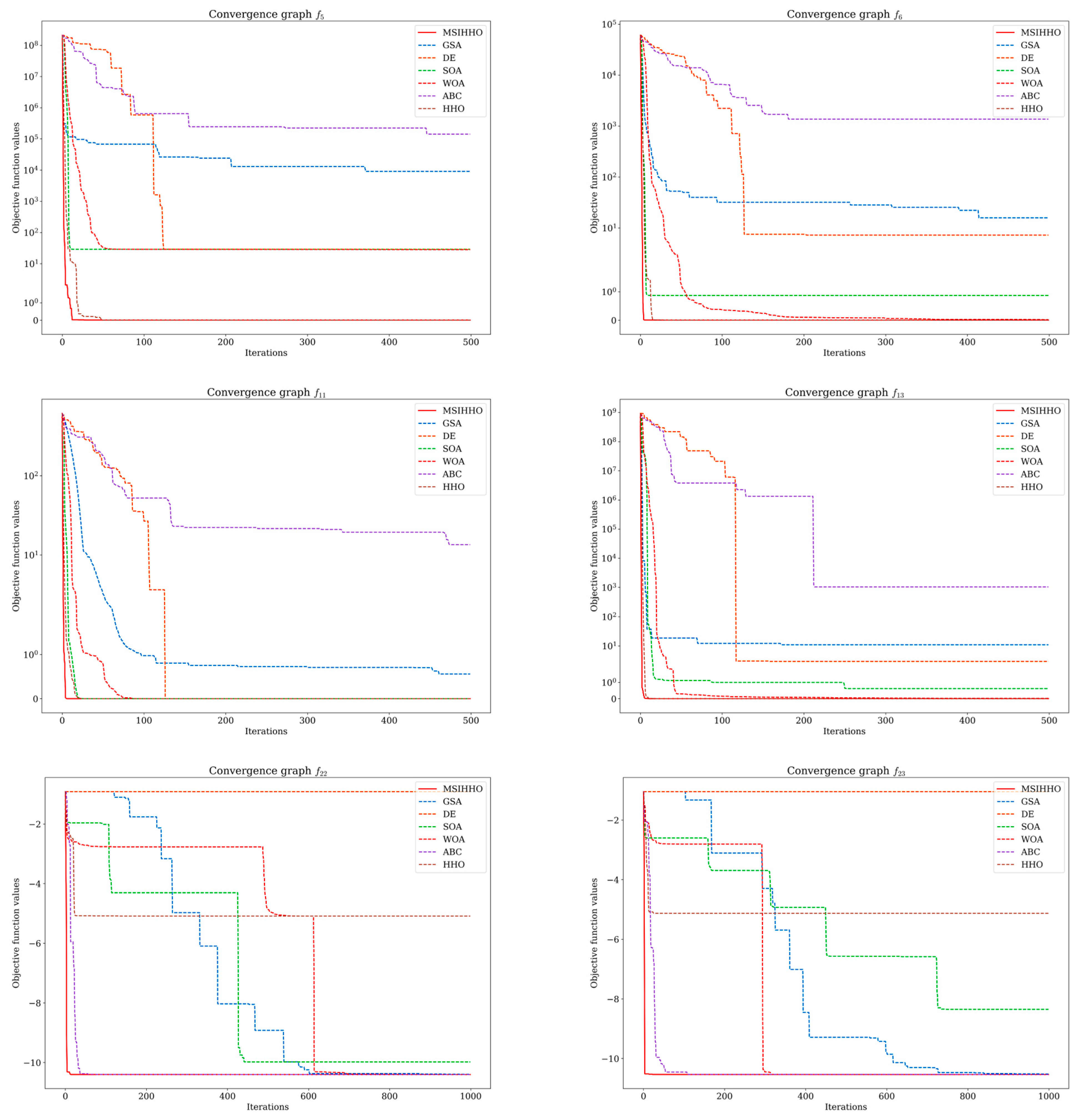
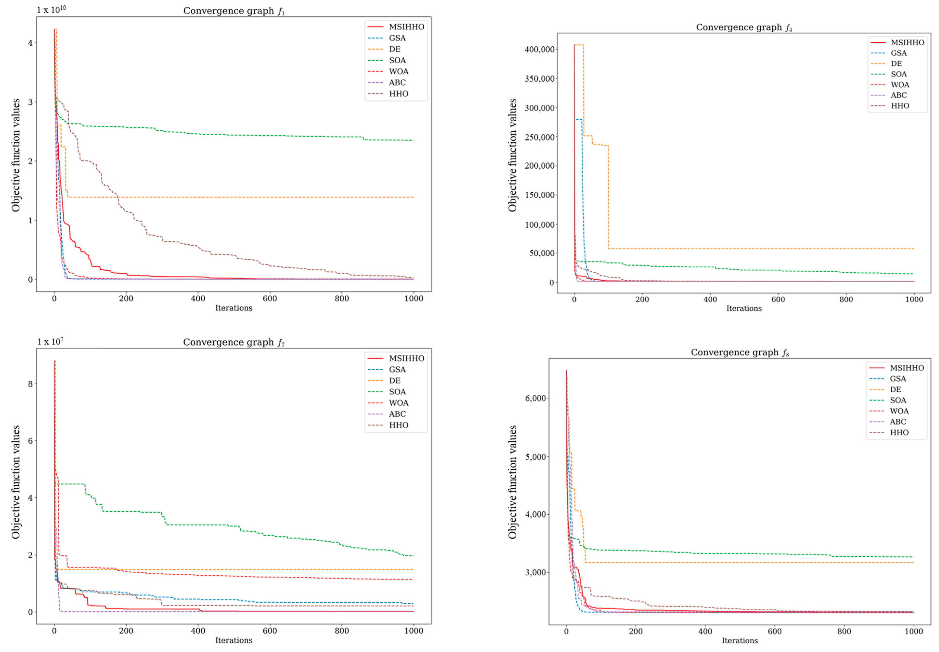
4.4. Iterative Curve
To further compare the convergence performance of MSI-HHO with that of other algorithms, we choose six and four functions from the two datasets mentioned above, respectively, to draw the convergence curves, as shown in Figure 6 and Figure 7. In consideration of the diverse types of test functions, we make selections from each type to create visualizations for analysis purposes. These selections are made to ensure a representative coverage of the different function types within each dataset.
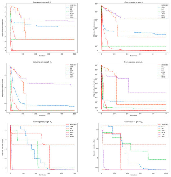
Figure 6.
The convergence graphs of the 23 classical benchmark functions.
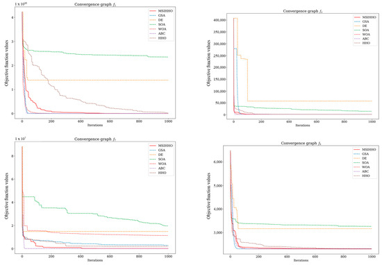
Figure 7.
The convergence graphs of the IEEE CEC 2020 benchmark functions.
As shown in Figure 6 and Figure 7, the convergence speed and search accuracy of different algorithms show significant variations. Throughout the 23 classical benchmark functions and the CEC 2020 benchmark functions, MSI-HHO consistently achieves convergence within the fewest number of iterations while successfully searching for the global optimal solution, exhibiting noteworthy exploration and exploitation capabilities. These findings provide further evidence for the effectiveness of the three enhancement strategies proposed in this study, which significantly improve the performance of HHO.
5. Conclusions
In this paper, we propose the MSI-HHO algorithm, which adopts three strategies to improve the performance of the standard HHO algorithm, i.e., inverted S-shaped escape energy, a stochastic learning mechanism based on Gaussian mutation, and refracted opposition-based learning. Furthermore, to assess the effectiveness of the proposed algorithm, a comprehensive evaluation is conducted by comparing it with the standard HHO algorithm and five other well-known search algorithms, i.e., GSA, DE, SOA, WOA, and ABC. Numerous simulation experiments are carried out on both the 23 classical benchmark functions and the IEEE CEC 2020 benchmark functions. The experimental results are analyzed by using two widely used non-parametric test methods, including the Wilcoxon signed-rank test and Friedman test. Finally, the convergence curves of the algorithms are generated to facilitate a comprehensive analysis of their convergence and optimization capabilities. Based on the aforementioned results and analysis, it is proved that our proposed MSI-HHO has a significant performance improvement over HHO and the other five algorithms.
In the future, we intend to include recently proposed advanced metaheuristic optimization algorithms in comparative experiments to further evaluate the performance of our proposed algorithm. Additionally, beyond numerical experiments, we will apply our algorithm to a wider range of real-world engineering optimization problems to comprehensively assess its effectiveness and robustness. While our method has achieved satisfactory solution accuracy, it has also resulted in relatively higher computational costs. Consequently, we will continue to explore further optimizations for the algorithm, starting from the specific procedures, in order to strike a better balance between search accuracy and computational efficiency.
Author Contributions
Conceptualization, H.W.; Funding acquisition, J.T.; Methodology, H.W. and Q.P.; Project administration, J.T.; Supervision, J.T. and Q.P.; Validation, H.W. and Q.P.; Visualization, H.W.; Writing—original draft, H.W.; Writing—review and editing, J.T. and Q.P. All authors have read and agreed to the published version of the manuscript.
Funding
This work was supported by the National Natural Science Foundation of China, grant number 62073330.
Data Availability Statement
All data generated or analyzed during this study are available from the corresponding author on reasonable request.
Conflicts of Interest
The authors declare that they have no conflicts of interest.
References
- Yaşa, E.; Aksu, D.T.; Özdamar, L. Metaheuristics for the Stochastic Post-Disaster Debris Clearance Problem. IISE Trans. 2022, 54, 1004–1017. [Google Scholar] [CrossRef]
- Simpson, A.R.; Dandy, G.C.; Murphy, L.J. Genetic Algorithms Compared to Other Techniques for Pipe Optimization. J. Water Resour. Plann. Manag. 1994, 120, 423–443. [Google Scholar] [CrossRef]
- Tang, J.; Liu, G.; Pan, Q. A Review on Representative Swarm Intelligence Algorithms for Solving Optimization Problems: Applications and Trends. IEEE/CAA J. Autom. Sin. 2021, 8, 1627–1643. [Google Scholar] [CrossRef]
- Ezugwu, A.E.; Shukla, A.K.; Nath, R.; Akinyelu, A.A.; Agushaka, J.O.; Chiroma, H.; Muhuri, P.K. Metaheuristics: A Comprehensive Overview and Classification along with Bibliometric Analysis. Artif. Intell. Rev. 2021, 54, 4237–4316. [Google Scholar] [CrossRef]
- Kirkpatrick, S.; Gelatt, C.D.; Vecchi, M.P. Optimization by Simulated Annealing. Science 1983, 220, 671–680. [Google Scholar] [CrossRef] [PubMed]
- Kennedy, J.; Eberhart, R. Particle Swarm Optimization. In Proceedings of the ICNN’95-International Conference on Neural Networks, Perth, WA, Australia, 27 November–1 December 1995; IEEE: Piscataway, NJ, USA, 1995; Volume 4, pp. 1942–1948. [Google Scholar]
- Holland, J.H. Adaptation in Natural and Artificial Systems: An Introductory Analysis with Applications to Biology, Control, and Artificial Intelligence, 1st ed.; Complex adaptive systems; MIT Press: Cambridge, MA, USA, 1992; ISBN 978-0-262-08213-6. [Google Scholar]
- Mirjalili, S.; Mirjalili, S.M.; Lewis, A. Grey Wolf Optimizer. Adv. Eng. Softw. 2014, 69, 46–61. [Google Scholar] [CrossRef]
- Storn, R.; Price, K. Differential Evolution—A Simple and Efficient Heuristic for Global Optimization over Continuous Spaces. J. Glob. Optim. 1997, 11, 341–359. [Google Scholar] [CrossRef]
- Beyer, H.-G.; Schwefel, H.-P. Evolution Strategies—A Comprehensive Introduction. Nat. Comput. 2002, 1, 3–52. [Google Scholar] [CrossRef]
- Artificial Intelligence through Simulated Evolution. In Evolutionary Computation; IEEE: Piscataway, NJ, USA, 2009; ISBN 978-0-470-54460-0.
- Rashedi, E.; Nezamabadi-pour, H.; Saryazdi, S. GSA: A Gravitational Search Algorithm. Inf. Sci. 2009, 179, 2232–2248. [Google Scholar] [CrossRef]
- Yadav, A. AEFA: Artificial Electric Field Algorithm for Global Optimization. Swarm Evol. Comput. 2019, 48, 93–108. [Google Scholar] [CrossRef]
- Geem, Z.W.; Kim, J.H.; Loganathan, G.V. A New Heuristic Optimization Algorithm: Harmony Search. Simulation 2001, 76, 60–68. [Google Scholar] [CrossRef]
- Rao, R.V.; Savsani, V.J.; Vakharia, D.P. Teaching–Learning-Based Optimization: A Novel Method for Constrained Mechanical Design Optimization Problems. Comput.-Aided Des. 2011, 43, 303–315. [Google Scholar] [CrossRef]
- Das, B.; Mukherjee, V.; Das, D. Student Psychology Based Optimization Algorithm: A New Population Based Optimization Algorithm for Solving Optimization Problems. Adv. Eng. Softw. 2020, 146, 102804. [Google Scholar] [CrossRef]
- Dhiman, G.; Kumar, V. Seagull Optimization Algorithm: Theory and Its Applications for Large-Scale Industrial Engineering Problems. Knowl.-Based Syst. 2019, 165, 169–196. [Google Scholar] [CrossRef]
- Mirjalili, S.; Lewis, A. The Whale Optimization Algorithm. Adv. Eng. Softw. 2016, 95, 51–67. [Google Scholar] [CrossRef]
- Karaboga, D.; Basturk, B. A Powerful and Efficient Algorithm for Numerical Function Optimization: Artificial Bee Colony (ABC) Algorithm. J. Glob. Optim. 2007, 39, 459–471. [Google Scholar] [CrossRef]
- Heidari, A.A.; Mirjalili, S.; Faris, H.; Aljarah, I.; Mafarja, M.; Chen, H. Harris Hawks Optimization: Algorithm and Applications. Future Gener. Comput. Syst. 2019, 97, 849–872. [Google Scholar] [CrossRef]
- Zou, T.; Wang, C. Adaptive Relative Reflection Harris Hawks Optimization for Global Optimization. Mathematics 2022, 10, 1145. [Google Scholar] [CrossRef]
- Shehabeldeen, T.A.; Elaziz, M.A.; Elsheikh, A.H.; Zhou, J. Modeling of Friction Stir Welding Process Using Adaptive Neuro-Fuzzy Inference System Integrated with Harris Hawks Optimizer. J. Mater. Res. Technol. 2019, 8, 5882–5892. [Google Scholar] [CrossRef]
- Rodríguez-Esparza, E.; Zanella-Calzada, L.A.; Oliva, D.; Heidari, A.A.; Zaldivar, D.; Pérez-Cisneros, M.; Foong, L.K. An Efficient Harris Hawks-Inspired Image Segmentation Method. Expert Syst. Appl. 2020, 155, 113428. [Google Scholar] [CrossRef]
- Chen, H.; Jiao, S.; Wang, M.; Heidari, A.A.; Zhao, X. Parameters Identification of Photovoltaic Cells and Modules Using Diversification-Enriched Harris Hawks Optimization with Chaotic Drifts. J. Clean. Prod. 2020, 244, 118778. [Google Scholar] [CrossRef]
- Amiri Golilarz, N.; Gao, H.; Demirel, H. Satellite Image De-Noising With Harris Hawks Meta Heuristic Optimization Algorithm and Improved Adaptive Generalized Gaussian Distribution Threshold Function. IEEE Access 2019, 7, 57459–57468. [Google Scholar] [CrossRef]
- Gezici, H.; Livatyalı, H. Chaotic Harris Hawks Optimization Algorithm. J. Comput. Des. Eng. 2022, 9, 216–245. [Google Scholar] [CrossRef]
- Tizhoosh, H.R. Opposition-Based Learning: A New Scheme for Machine Intelligence. In Proceedings of the International Conference on Computational Intelligence for Modelling, Control and Automation and International Conference on Intelligent Agents, Web Technologies and Internet Commerce (CIMCA-IAWTIC’06), Vienna, Austria, 28–30 November 2005; IEEE: Piscataway, NJ, USA, 2005; Volume 1, pp. 695–701. [Google Scholar]
- Sahoo, S.K.; Saha, A.K.; Nama, S.; Masdari, M. An Improved Moth Flame Optimization Algorithm Based on Modified Dynamic Opposite Learning Strategy. Artif. Intell. Rev. 2023, 56, 2811–2869. [Google Scholar] [CrossRef]
- Rahnamayan, S.; Tizhoosh, H.R.; Salama, M.M.A. Opposition-Based Differential Evolution. IEEE Trans. Evol. Computat. 2008, 12, 64–79. [Google Scholar] [CrossRef]
- Xu, Y.; Yang, Z.; Li, X.; Kang, H.; Yang, X. Dynamic Opposite Learning Enhanced Teaching–Learning-Based Optimization. Knowl.-Based Syst. 2020, 188, 104966. [Google Scholar] [CrossRef]
- Cao, D.; Xu, Y.; Yang, Z.; Dong, H.; Li, X. An Enhanced Whale Optimization Algorithm with Improved Dynamic Opposite Learning and Adaptive Inertia Weight Strategy. Complex Intell. Syst. 2023, 9, 767–795. [Google Scholar] [CrossRef]
- Wang, Y.; Jin, C.; Li, Q.; Hu, T.; Xu, Y.; Chen, C.; Zhang, Y.; Yang, Z. A Dynamic Opposite Learning-Assisted Grey Wolf Optimizer. Symmetry 2022, 14, 1871. [Google Scholar] [CrossRef]
- Wang, H.; Wu, Z.; Rahnamayan, S.; Liu, Y.; Ventresca, M. Enhancing Particle Swarm Optimization Using Generalized Opposition-Based Learning. Inf. Sci. 2011, 181, 4699–4714. [Google Scholar] [CrossRef]
- Long, W.; Wu, T.; Cai, S.; Liang, X.; Jiao, J.; Xu, M. A Novel Grey Wolf Optimizer Algorithm with Refraction Learning. IEEE Access 2019, 7, 57805–57819. [Google Scholar] [CrossRef]
- Long, W.; Wu, T.; Jiao, J.; Tang, M.; Xu, M. Refraction-Learning-Based Whale Optimization Algorithm for High-Dimensional Problems and Parameter Estimation of PV Model. Eng. Appl. Artif. Intell. 2020, 89, 103457. [Google Scholar] [CrossRef]
- Adegboye, O.R.; Deniz Ülker, E. Hybrid Artificial Electric Field Employing Cuckoo Search Algorithm with Refraction Learning for Engineering Optimization Problems. Sci. Rep. 2023, 13, 4098. [Google Scholar] [CrossRef] [PubMed]
- Pan, Q.; Tang, J.; Lao, S. EDOA: An Elastic Deformation Optimization Algorithm. Appl. Intell. 2022, 52, 17580–17599. [Google Scholar] [CrossRef]
- Derrac, J.; García, S.; Molina, D.; Herrera, F. A Practical Tutorial on the Use of Nonparametric Statistical Tests as a Methodology for Comparing Evolutionary and Swarm Intelligence Algorithms. Swarm Evol. Comput. 2011, 1, 3–18. [Google Scholar] [CrossRef]

Disclaimer/Publisher’s Note: The statements, opinions and data contained in all publications are solely those of the individual author(s) and contributor(s) and not of MDPI and/or the editor(s). MDPI and/or the editor(s) disclaim responsibility for any injury to people or property resulting from any ideas, methods, instructions or products referred to in the content. |
© 2024 by the authors. Licensee MDPI, Basel, Switzerland. This article is an open access article distributed under the terms and conditions of the Creative Commons Attribution (CC BY) license (https://creativecommons.org/licenses/by/4.0/).