CNVbd: A Method for Copy Number Variation Detection and Boundary Search

Abstract

Copy number variation (CNV) has been increasingly recognized as a type of genomic/genetic variation that plays a critical role in driving human diseases and genomic diversity. CNV detection and analysis from cancer genomes could provide crucial information for cancer diagnosis and treatment. There still remain considerable challenges in the control-free calling of CNVs accurately in cancer analysis, although advances in next-generation sequencing (NGS) technology have been inspiring the development of various computational methods. Herein, we propose a new read-depth (RD)-based approach, called CNVbd, to explore CNVs from single tumor samples of NGS data. CNVbd assembles three statistics drawn from the density peak clustering algorithm and isolation forest algorithm based on the denoised RD profile and establishes a back propagation neural network model to predict CNV bins. In addition, we designed a revision process and a boundary search algorithm to correct the false-negative predictions and refine the CNV boundaries. The performance of the proposed method is assessed on both simulation data and real sequencing datasets. The analysis shows that CNVbd is a very competitive method and can become a robust and reliable tool for analyzing CNVs in the tumor genome.

1. Introduction

Copy number variation (CNV) refers to a type of intermediate-scale structural variation with copy number changes and has been increasingly recognized as having a significant effect on human genomic diversity, tumorigenesis, and the pathogenesis of multiple inherited genetic disorders and intellectual disability [1,2,3,4]. CNVs can be insertions, deletions, duplications, inversions, translocations, transversions, or more complicated forms involving DNA segments ranging in size from hundreds of base pairs to several megabases or even beyond. It has been estimated that CNVs occur in more than 12% of the human genome as passenger mutations or covering functional genes of human cancer and other complex diseases [5]. Additionally, a large part of CNVs exist in the protein-coding regions and thus influence the concerned gene expressions [6]. Therefore, CNV detection is fundamental for the comprehensive genetic analysis of human diseases and a better understanding of genome evolution.

The read-depth (RD)-based methods for CNV detection have been proven to be the most versatile and most widely used for both whole-genome and whole-exome sequencing data [7,8] among the varieties of computational tools that emerged along with the massive and high-resolution data generated by the next-generation sequencing (NGS) technologies. Moreover, the RD-based approaches are not affected by the short read length and discontinuous targeted regions across the genome and have the potential to accurately estimate the absolute copy numbers [9]. CNVs can be divided into two groups: copy number gain and copy number loss. A gain should show higher RD intensity than expected, while a loss shows the opposite [10]. The RD strategies work under the assumption that the depth of coverage is approximately proportional to the copy number of that location [11]. The depth of coverage at a location can be represented by the read count (RC), i.e., the number of reads mapped to the location. However, there are some factors, such as low sequencing depth, GC content bias, mappability bias, experimental noise, and alignment errors, that reduce base pair resolution and distort the relationship between the RC and the copy number. This necessitates a procedure of binning along the genome and a process of GC bias correction, which have become an essential part of the RD-based approaches for CNV detection [12]. Generally, the pipeline of CNV detection based on RD includes the following major steps: quality control of raw reads, alignment of reads to the reference genome, data preprocessing (binning, RD calculation, and GC bias or other bias correction across the RDs), and CNV calling (inferring gain or loss by developing a statistical model or machine learning algorithms based on the RD profile and other alignment information). Although these general operations of the RD-based approaches enhance the possibility of detecting large CNVs and also work for complicated genomic areas, they fail to obtain accurate CNV boundaries, which increases the false-positive rate.

A large number of methods under the RD-based framework have been developed for detecting CNVs of different sizes and types from various viewpoints. Conventional detection approaches construct statistical models that usually presuppose a probability distribution followed by RDs and forecast CNVs using hypothesis-based analytical techniques. For instance, SegSeq [13] and ReadDepth [14] adopt models based on Poisson, Gaussian, and negative binomial distributions. There are also many other methods that implement a segmentation process after various bias corrections (e.g., FREEC [15], CNVnator [16], CNVkit [17], and iCopyDAV [18]) or apply different algorithms to infer the copy numbers (e.g., CopywriteR [19], GROM-RD [20], and SeqCNV [21]) in order to detect the CNVs as well as the breakpoints, i.e., the start/end boundaries of predicted CNVs. FREEC and CNVnator achieve fine performance and are therefore often used for comparison with a newly developed method. Currently, CNVs are mostly regarded as outlier events to be analyzed from the RD profile since the CNV regions only account for a small part of the genome. For example, CNV-LOF [22], CNV-KOF [23], and IhybCNV [24] adopt different outlier factors to calculate anomaly scores and determine CNVs by applying a boxplot or binary clustering model. Along with the development of machine learning, models based on classification, regression, neural networks, or clustering are adopted by CNV detection methods, including AluScanCNV2 [25], CNV_IFTV [26], CNV-RF [27], and dpCNV [28], and so on. However, most such types of methods are not able to locate the precise breakpoints of CNVs unless specific treatment is taken. Nonetheless, due to the intrinsic complexity of the genome and the existence of various systemic noises, there still remain many challenges associated with the analysis of NGS data for CNVs. Therefore, it requires more feasible and reliable strategies for the detection of CNVs from NGS data.

We present a new method called CNVbd to detect CNVs from single tumor samples of NGS data. CNVbd generates a RD profile through a binning procedure and GC content corrections. Based on the RD file, it calculates three types of outlier scores derived from the density peak clustering algorithm and the isolation forest algorithm for each genome bin. Combining RDs with the three statistics, it then trains a back propagation (BP) neural network model to predict CNV bins. In addition, CNVbd implements a revision process specifically designed for connecting the successive CNV pieces so as to improve the false negative rate, as well as a boundary search algorithm for locating the breakpoints. To validate our proposed method, we first compare its performance on simulation data to four peer methods. We also apply our proposed boundary search algorithm to the peer methods in order to compare their boundary accuracy. We further verified the CNVbd method on real tumor samples. The comparative study demonstrates the superiority of CNVbd over the other approaches, and we expect it to become a routine approach for the detection of CNVs from single tumor samples of NGS data.

2. Methods

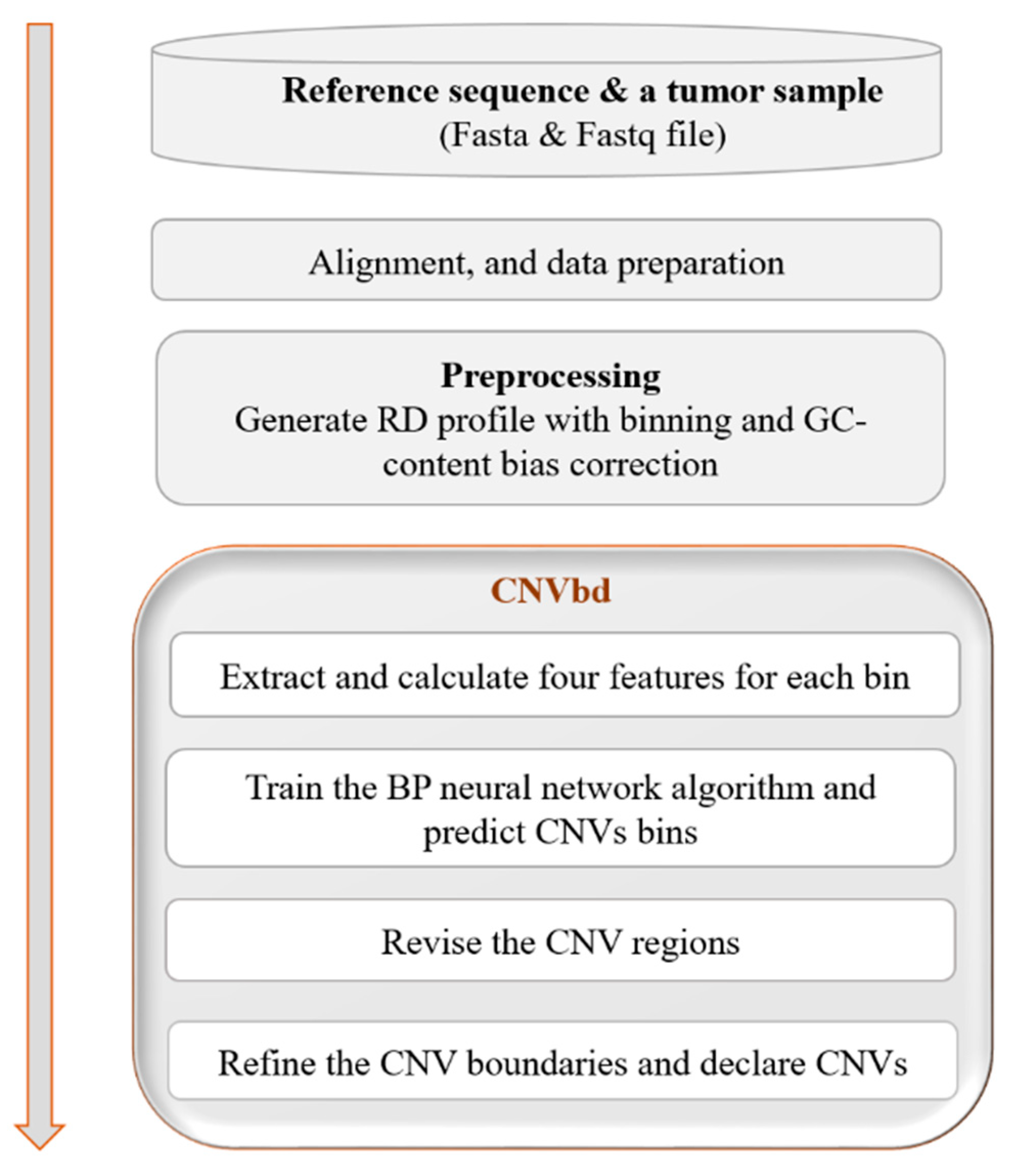
2.1. Overview of CNVbd

CNVbd is based on the RD approach, which does not require a control-matched sample. The flowchart of CNVbd is illustrated in Figure 1. Firstly, a sequenced sample (i.e., a Fastq file) is aligned to the reference sequence (i.e., an Hg38 Fasta file) by BWA [29], which is currently one of the most popular alignment tools. This process produces the SAM/BAM file, through which the RC profile is generated with SAMtools [30]. The RC values of the value-lost and “N” positions are filled with zeros to obtain a complete and workable RC profile. Then, an RD profile is generated by dividing the complete RC profile into bins and performing a GC bias correction process. With the RD profile, CNVbd begins to detect CNVs through four steps. In the first step, four CNV-related features are extracted or calculated. In the second step, the BP neural network algorithm is trained based on the four features to predict the gain or loss CNV bins. In the third step, a designed revision process is applied to certain CNV regions. In the last step, a boundary search algorithm is implemented to refine the CNV boundaries, and all CNVs are finally declared. The CNVbd program is written in Python and is freely available at https://github.com/BDanalysis/CNVbd, accessed on 8 May 2023. This software is easy to install and configure. Please refer to the above website for the specific usage and requirements of this method. The principle and implementation for each of the steps are described in detail in the following subsections.

2.2. Preprocessing

This step includes drawing up the RC profile and generating the RD profile by binning and correcting the GC content bias. The complete RC profile is divided into non-overlapping bins of a fixed size along the genome, and the reads falling into each bin are counted, which is a strategy to capture the local variation signals. The size was set to 1500 bp here in order to provide a relatively loose range for the subsequence boundary search. For each bin, a mean RC was computed to attain its RD value. The ratio of the number of bases “G” and “C” to the number of all the bases in a bin is known as the GC content. GC content bias is caused by the unequal distribution of reads during the polymerase chain reaction [31], which has an impact on the RD values.

In this paper, GC content bias was corrected for the RD profile following the method introduced in [26], as shown in Equation (1):

$$r_i=\frac{\overline{r}-r_e}{{\overline{r}}_{gc}-r_e}·{\tilde{r}}_i$$

(1)

where ${\tilde{r}}_i$ represents the raw RD of the i-th bin, $\overline{r}$ represents the average RD across all bins, ${\overline{r}}_{gc}$ represents the average RD across those bins with a similar GC fraction to the i-th bin, and $r_e$ represents the average error-mapped read count across the genome that can be estimated according to the mapping information recorded in the SAM file using SAMtools. The result $r_i$ is the corrected RD value of the i-th bin. Thus, a corrected RD profile was obtained.

2.3. Extract and Calculate CNV-Related Features

Extracting effective features that capture the signature of CNVs is one of the key steps to detect CNVs, which will directly affect the detection accuracy. For each bin, we extracted four features, i.e., read-depth (RD), local density (LD), minimum distance (MD), and IFTV deep (ID), as shown in

Table 1. Description of the extracted features.

Feature	Description
Read-depth (RD), $r_i$	The corrected RD for each bin
Local density (LD), ${\rho }_i$	The number of points that are closer than the cutoff distance to point $i$
Minimum distance (MD), ${\delta }_i$	The minimum distance between the point $i$ and any other point with higher density
IFTV deep (ID), hi	The isolation forest deep, i.e., the average depth of $r_i$ in all iTrees

, with their corresponding meanings described. The RD was prepared. The other three features were measured based on the RD.

2.3.1. Calculate the Values of the Features LD and MD

The LD and MD are two quantities introduced and mainly used in clustering by fast search and find of density peaks [32] for outlier detection. The local density ${\rho }_i$ is equal to the number of points that are within a cutoff distance of the i-th bin point, calculated using Equation (2):

$${\rho }_i=\sum _j\mathcal{X}\left(d_{ij}-d_c\right)$$

(2)

where $\mathcal{X}\left(x\right)=1$ if $x<0$ and $\mathcal{X}\left(x\right)=0$; otherwise, $d_c$ is the cutoff distance, and $d_{ij}=\sqrt{{(r_i-r_j)}^2+{(i-j)}^2}$ represents the Euclidean distance between the $i$-th and $j$-th bin points. The minimum distance ${\delta }_i$ denotes the distance from the $i$-th bin point to its nearest higher density bin point, shown as Equation (3):

$${\delta }_i=\underset{j:{\rho }_j>{\rho }_i}{\min }{d}_{ij}$$

(3)

For the point with the highest density, take ${\delta }_i=d_{ij}$. An example is shown in Figure 2, where $\mathrm{L}\mathrm{D}=5$, $d_c$ equals the length of the dashed line and MD equals the length of the brown dotted line. Both quantities only depend on the distance $d_{ij}$. An outlier is supposed to have a lower LD value and a larger MD value than normal points.

2.3.2. Calculate the Value of the Feature ID

An isolated forest is a collection of isolated trees (iTrees). Each iTree is a binary tree classifier, with every leaf being a class, which is trained by Algorithm 1 and can be referred to [26]. The deep level of a value in an iTree is defined as the path length from the root to the leaf that the value belongs to. For a clear understanding of Algorithm 1, an example of training an iTree on a set of ten values is presented in Figure 3, where the bold numbers are the randomly selected values following step (3).

Algorithm 1. Training an iTree.
(1)	$\mathrm{Take}\mathrm{a}\mathrm{subsample}\mathrm{X}\mathrm{of}{N}_n$ bins from all the bins;
(2)	Let Q be the list of RD values in X;
(3)	Randomly select a value $q\mathsf{ϵ}[\min \left(Q\right),\mathrm{m}\mathrm{a}\mathrm{x}(Q\left)\right]$ as a root or sub-root and divide X into two subsets, the left side and the right side:               $X_l=\left\{xϵX|Q\left(x\right)<q\right\}$               $X_r=\left\{xϵX|Q\left(x\right)\ge q\right\}$ where Q$\left(\mathrm{x}\right)\mathrm{is}\mathrm{the}\mathrm{RD}\mathrm{value}\mathrm{of}\mathrm{bin}x$;
(4)	$\mathrm{Let}X=X_l$$\mathrm{or}X=X_r$;
(5)	$\mathrm{Repeat}\mathrm{steps}\left(2\right)\mathrm{to}\left(4\right)\mathrm{until}\left|X\right|\le 1$.

Since outliers take fewer steps to be classified, they have smaller deep values than normal values generally. The ID value $h_i$ of the i-th bin is equal to the mean depth of $r_i$ over all the iTrees, as shown by Equation (4):

$$h_i=E\left(h\left(r_i\right)\right)$$

(4)

Considering the large number of genome bins, the subsample size $N_n$ and the number of iTrees $N_t$ were both taken as 256 to assure convergence and obtain reliable detection of anomalies in the experiments.

2.4. Predict the CNV Bins by Training the BP Neural Network Algorithm

With the four features, we predicted the CNV bins by training the BP neural network algorithm [33]. The BP neural network is a well-known method of training a multilayer feedforward neural network and is applied to many fields due to its simple topology and good learning ability. It consists of three types of layers: input, hidden, and output. The core idea of the algorithm is that it adjusts the weights between neurons through back propagation, which continuously reduces errors and thus optimizes output. Here, the BP neural network we use contains four layers: one input, two hidden, and one output, as shown in Figure 4. The input layer consists of 4 neurons corresponding to the 4 features. The two hidden layers consist of 25 neurons and 10 neurons, respectively, according to our extensive testing. The parameters of the architecture were determined by extensive testing. The number of hidden layers was tested from 1 to 5, and it turned out that two hidden layers were enough to accomplish the classification task and did not cause overfitting. All the combinations of the number of neurons in the two layers from the set {5, 10, 15, 20, 25, 30} are tested, and (25, 10) works best. For the hidden layers, we used the Rectified Linear Unit (ReLU) function [34] as their activation function (Equation (5)) for good stability and fast convergence. As for the output layer, we used the Softmax function as its activation function (Equation (6)), which can effectively display the multi-classification results in the form of probability.

$$f(W^{T}x+b)=\max (0,W^{T}x+b)$$

(5)

$$f(W^{T}x+b)=\frac{e^{W^{T}x+b}}{\sum _i({W_i}^{T}x+b_i)}$$

(6)

Here, $W$ denotes the weight matrix between two layers, $b$ denotes the corresponding biases, and $x$ denotes the neuron input vector from the previous layer. Thus $y=W^{T}x+b$ in Equation (6) is the output, and $W_i$ is the $i$-th column of $W$.

The output layer consists of three neurons corresponding to predicted normal or two types of CNV bins (i.e., gain or loss) according to their RD values. A detected CNV region is declared a loss if its RD value is lower than the mean RD over all the bins; otherwise, it is a gain. Since real samples are generally impure, the model is trained on simulated datasets incorporating multiple tumor purities for well-rounded generalization. The datasets are divided into two parts according to 4:1 for training and validation, respectively. The model can also be trained on real sequencing samples with ground-truth CNVs.

2.5. Revise the CNV Regions

In this section, we design a revision process to reduce the false negatives, trying to pick up the local signals that could not be captured by the prediction model, especially for data with low sequencing coverage. The previous step predicted each bin in the form of gain, loss, or normal. A segment of continuous gain, loss, or normal bins is called a gain, loss, or normal block, respectively. A normal block consisting of at least ten bins is regarded as big; otherwise, it is small. Now we can divide the sample sequence into CNV regions by big normal blocks. The CNV regions are classified into two categories: the continuous type, which is entirely a CNV block, and the alternate type, which consists of CNV blocks and small normal blocks, as shown in Figure 5. The revision process aims at the alternate CNV regions with a proportion of CNV bins above a certain level because false predictions exist with a higher possibility in these regions than in the continuous ones.

In the revision process, each normal bin will be compared with its nearby bins, since adjacent bins across the genome are usually positionally correlated from the perspective of copy number [5,35]. The revision process is implemented on an alternate CNV region when the proportion $P$ of CNV bins is greater than the threshold $\tau$. For each CNV block in a region, the revision process runs over normal bins, first on the left side, then on the right side, from near to far. For each CNV block, denote by $D_L$ and $D_R$ the left and right base values, respectively, calculated by Equations (7) and (8):

$$D_L=(1-P)·{\overline{RD}}_{CNV}+P·{\overline{RD}}_{LN}$$

(7)

$$D_R=(1-P)·{\overline{RD}}_{CNV}+P·{\overline{RD}}_{RN}$$

(8)

where ${\overline{RD}}_{CNV}$ is the average RD value of all the bins in the CNV block, and ${\overline{RD}}_{LN}$ (or ${\overline{RD}}_{RN}$) is the average RD value of the nearest ten normal bins contained in the left (or right) big normal block of the CNV region. Each normal bin between two consecutive CNV blocks is revised twice by comparing its RD value, respectively, to $D_R$ as the right side of the left CNV block and to $D_L$ as the left side of the right CNV block. A bin will be finally declared to be a CNV bin if it gets revised at least once, i.e., the RD value of the bin exceeds $D_L$ or $D_R$. The revision process for a normal bin on the left side of a CNV block is described in Algorithm 2. The revision process for a bin on the right side of a CNV block is similar, except that ${\overline{RD}}_{RN}$ and $D_R$ are used accordingly. Considering that the amplitudes resulting from copy number gains and losses are usually unsymmetrical [36], the threshold $\tau$ for a gain region or a loss region is set to be different, respectively, 0.2 or 0.4, which would be the best according to our extensive testing.

Algorithm 2. Revise the normal bins on the left side of a CNV block.
(1)	Calculate the CNV proportion $P$ in the region;
(2)	If $P\ge \tau$, then calculate $D_L$; otherwise, keep bin $i$ as normal and quit.
(3)	If $r_i\ge D_L$ for a gain region (or $r_i\le D_L$ for a loss region), then bin $i$ is revised to be a CNV gain (or loss); otherwise, keep bin $i$ as normal and quit.
(4)	Recalculate ${\overline{RD}}_{CNV}$ and let $i=i-1$.
(5)	Repeat steps (2) to (4) until there is no normal bin left on the left side.

To understand the revision algorithm more clearly, please see the example shown in Figure 6. The revision process of bins $i$ and $i+1$ were completed by the following two big steps:

• For the left gain block, the revision process starts at bin $i$. (1) Calculate $P=4/6\approx 0.66>0.2$. Assume that ${\overline{RD}}_{LN}=4.5$ and ${\overline{RD}}_{RN}=4.2$ have been calculated. (2) Calculate ${\overline{RD}}_{CNV}=(8+9)/2=8.5$ and $D_R\approx 0.34·8.5+0.66·4.2=5.66$. It can be seen that $r_i=5<D_R$, so the bin $i$ stays normal. In this case, the revision for the right side of the left gain block is over. Bin $i+1$ also stays normal.
• For the right gain block, the revision process starts at bin $i+1$. (1) Calculate ${\overline{RD}}_{CNV}=(8+8)/2=8$ and $D_L\approx 0.34·8+0.66·4.5=5.49$. It can be seen that $r_{i+1}=6>D_L$, so bin $i+1$ is revised to be a gain. (2) For bin i, recalculate ${\overline{RD}}_{CNV}=(8+8+6)/3\approx 7.33$ and $D_L\approx 0.34·7.33+0.66·4.5=5.46$. Since $r_i=5<D_L$, bin $i$ stays normal.

Finally, bin $i$ still stays normal, and bin $i+1$ is revised to be a gain.

2.6. Refine the CNV Boundary and Declare CNVs

Most of the existing methods of detecting CNV using bin dividing take the boundaries of end-bins as the CNV boundaries by default, which is hardly in line with reality. Therefore, we made an effort to refine the CNV boundary based on the previous predictions. After performing revisions, many normal bins become CNV bins, so that some regions of the alternate type become continuous types. However, each CNV region keeps the values of ${\overline{RD}}_{LN}$ and ${\overline{RD}}_{RN}$ unchanged. We designed a boundary search (BDS) algorithm to find the ends of every CNV block. Suppose the left (or right) boundary is inside the border region covering the left-end (or right-end) CNV bin and its adjacent normal bin. The algorithm is implemented in the region by the idea of dichotomy, i.e., splitting the search region in half every time until the scope reduces to a single base that will be considered the boundary. For example, to search the left boundary of a gain block, the process is as shown in Algorithm 3, which starts with the left-end CNV-bin and its adjacent normal bin, denoted by ${\mathrm{b}\mathrm{i}\mathrm{n}}_1$ and ${\mathrm{b}\mathrm{i}\mathrm{n}}_2$, respectively. The iteration process is driven by repeatedly subdividing two bins into four smaller bins and choosing two of them to narrow the search by comparing the RD values of the sub-bins to the base value $\mathrm{R}$.

Algorithm 3. The left boundary search for a gain block.
(1)	Divide ${\mathrm{b}\mathrm{i}\mathrm{n}}_1$ and ${\mathrm{b}\mathrm{i}\mathrm{n}}_2$ in half into four sub-bins: ${\mathrm{b}\mathrm{i}\mathrm{n}}_{\mathrm{A}}$, ${\mathrm{b}\mathrm{i}\mathrm{n}}_{\mathrm{B}}$, ${\mathrm{b}\mathrm{i}\mathrm{n}}_{\mathrm{C}}$, and ${\mathrm{b}\mathrm{i}\mathrm{n}}_{\mathrm{D}}$, from right to left.
(2)	Calculate $R=({\overline{RD}}_{LN}+{\overline{RD}}_{CNV})/2$ and the deviations ${\mathrm{d}}_{\mathrm{A}}={\mathrm{r}}_{\mathrm{A}}-\mathrm{R}$, ${\mathrm{d}}_{\mathrm{B}}={\mathrm{r}}_{\mathrm{B}}-\mathrm{R}$, ${\mathrm{d}}_{\mathrm{C}}={\mathrm{r}}_{\mathrm{C}}-\mathrm{R}$, and ${\mathrm{d}}_{\mathrm{D}}={\mathrm{r}}_{\mathrm{D}}-\mathrm{R}$ of the four sub-bins.
(3)	Choose two adjacent ones from the four sub-bins from right to left: take the first pair of sub-bins whose deviations change from non-negative to negative, if they exist; or take the leftmost two sub-bins, ${\mathrm{b}\mathrm{i}\mathrm{n}}_{\mathrm{C}}$ and ${\mathrm{b}\mathrm{i}\mathrm{n}}_{\mathrm{D}}$, if $\min \left({\mathrm{d}}_{\mathrm{A}},{\mathrm{d}}_{\mathrm{B}},{\mathrm{d}}_{\mathrm{C}},{\mathrm{d}}_{\mathrm{D}}\right)\ge 0$; otherwise, take the rightmost two bins, ${\mathrm{b}\mathrm{i}\mathrm{n}}_{\mathrm{A}}$ and ${\mathrm{b}\mathrm{i}\mathrm{n}}_{\mathrm{B}}$.
(4)	Replace ${\mathrm{b}\mathrm{i}\mathrm{n}}_1$ and ${\mathrm{b}\mathrm{i}\mathrm{n}}_2$ with the two sub-bins chosen in step (3), recalculate ${\overline{RD}}_{LN}$ and ${\overline{RD}}_{CNV}$, and repeat steps (1) to (3) until the lengths of the two sub-bins reduce to a single base.

As for searching the right boundary of a gain block, the algorithm is only different in step (3) in that the bin-choosing order is from left to right. With regard to a loss region, the BDS algorithm needs only to switch the positive and negative deviation conditions in step (3). For a better understanding of Algorithm 3, please see an example for the left boundary search of a gain block, as shown in Figure 7, where the first five iterations are presented. The values of ${\overline{RD}}_{LN}$, ${\overline{RD}}_{CNV}$, and $\mathrm{R}$ are recalculated during the third and fourth iterations. After the boundaries are refined, CNVs can be declared.

3. Results

To assess the effectiveness and reliability of our proposed method, we carried out experiments on both simulated and real datasets. CNVbd is trained on the simulation samples produced independently and is then tested on different simulation samples and applied to a collection of real sequencing samples. In the simulation study, with given ground-truth CNVs, we compared CNVbd to the two classic methods FREEC and CNVnator and to the other two methods CNV-IFTV and dpCNV that also, respectively, use features derived from isolation forest and density peak clustering algorithms in terms of precision, sensitivity, and F1 score. Here, precision is equal to the number of correct predictions divided by the total number of predictions, sensitivity is equal to the number of correct predictions divided by the total number of ground-truth CNVs, and the F1 score is the harmonic mean of sensitivity and precision. In a consistent experimental scenario, the trade-off between precision and sensitivity can explain the fairness of performance. To ensure that the comparison is as fair as possible, the default or recommended parameters of the compared methods were used during experiments. The effectiveness of the BDS algorithm was also verified on the simulated datasets. Moreover, to validate the practicability of CNVbd, we applied it to three real datasets without ground-truth CNVs obtained from the European Genome-phenome Archive (EGA) database. In this case, precision and sensitivity cannot be quantified directly. In order to evaluate the performance of CNVbd and the four peer methods on real sequencing samples, we analyzed their results by using the overlapping density score (ODS) proposed in [36].

3.1. Simulation Studies

CNVbd first needs to train a model to predict CNVs. The training datasets were generated by our previously developed simulation tool, IntSIM [37], which simulates broad and focal CNV events based on a class of statistical models with input parameters trained from real sequencing genomes. The mixed samples with coverage depths of 4× and 6× and tumor purities of 0.2~0.5 were used to train the prediction model. The testing datasets were produced by the popular simulation tool ART [38], which generates simulated sequencing reads by emulating the technology-specific sequencing process. Six scenarios were formed from various configurations of coverage depth (6× and 8×) and tumor purity (0.2, 0.4, and 0.6). Five replicated samples are produced in each configuration. Fourteen CNV regions, including six gains and four losses ranging from 10,000 to 300,000 bp, were simulated in each simulation replication. CNVbd and the four peer methods were implemented on the 30 samples for the performance comparison.

The comparative results of all five methods are illustrated in Figure 8, where the average values of precision, sensitivity, and F1 score (black curves) in different scenarios are presented. Here, one true positive is counted when it covers at least half of the region of one real CNV. We can observe that the efficiency of almost all the methods improves generally with the increase in tumor purity or coverage depth (Cov). For instance, the F1 score of the CNVbd method increases from around 0.4 to more than 0.8 when the tumor purity rises from 0.2 to 0.6. In terms of precision, the CNVbd obtains the top spot in one of the six simulation scenarios and ranks second inferior to the FREEC in three scenarios. In terms of recall, CNVbd is second only to CNVnator in all the simulation scenarios, followed by FREEC, CNV_IFTV, and dpCNV with their respective strong points. However, CNVbd yields the largest F1 score in five simulation configurations. As a summary of the above analysis and discussion, it is evident that CNVbd exhibits the best trade-off between precision and recall and shows stable performance in the detection of CNVs.

In order to verify the effectiveness of our proposed BDS algorithm, we compared the boundary deviations (from the true boundaries) of the common CNVs predicted by all five methods, as shown by the boxplots in Figure 9a,b, by taking the average value over all samples with the same coverage depth. The diagram uses the quartiles of the data as an indication of the spread, where the box lies between the upper and lower quartiles, the red solid line dividing the box into two and the blue dashed line represent the median and the mean value, respectively, the straight line extends from the ends of the box to the maximum and minimum values, and the round dots represent abnormal values. It can be seen that CNVnator performs best with both low and compact deviations, while CNVbd obtains the lowest minimum values for both coverages and the second lowest mean and median for coverages 6× and 8×, respectively. We also ran the BDS algorithm after the four peer methods and compared the boundary deviations, as shown in Figure 9c–f, including the comparison of the CNVbd methods before and after the performance of the BDS algorithm. It can be observed that the applications of the BDS algorithm indeed narrow the boundary deviations for all of the five methods in general, although here the changes are set to be limited to the length of one bin based on the previous predictions of a method. One may also choose more border bins as the searching region in the application of the BDS algorithm. Nevertheless, the above analysis shows that BDS is an effective algorithm for boundary refinement.

3.2. Application to Real Blood Samples

In view of the situation that the ground-truth CNVs provided by a database are usually incomplete (unless all CNVs are detected) and have inaccurate boundaries (unless specific treatments are taken for the precise breakpoints), this results in incorrect precision and sensitivity and thus unreliable comparisons. To evaluate the efficacy of our proposed method, CNVbd was applied to analyze three real sequencing samples without ground truth, namely EGAD00001000144_LC, EGAR00001004802_2053_1, and EGAR00001004836_2561_1, obtained from the EGA database (https://www.ebi.ac.uk/ega, accessed on 27 May 2015). These samples include a lung cancer sample and two ovarian cancer samples. We performed CNVbd on the 21st chromosome for each of the samples and made a comparison to the four peer single sample-based methods using the ODS calculated by Equation (9):

$$ODS=m_{cnv}.m_{cnv}^{\prime }$$

(9)

where $m_{cnv}$ represents the total number of overlapped events divided by the total number of compared methods, and $m_{cnv}^{\prime }$ represents the total number of overlapped events divided by the number of events predicted by itself. Considering the CNV boundaries, we calculate the ODS by counting each base in a CNV as an event. Thus, we actually count the total length instead of the number of CNVs detected by a method.

CNVnator retrieves the largest number of overlapping events in all three samples, but it also predicts the most non-overlapping events. Although CNVbd detects a slightly lower number of overlapping events than CNVnator, it detects zero non-overlapping events from two samples. FREEC detects a moderate number of overlapping events, and dpCNV obtains the least number of overlapping events in each sample. The overlapping events between the five methods performed on the lung cancer sample are described in Figure 10. The ODSs of the five methods for each sample are calculated and displayed in

Table 2. The ODSs of the five methods.

Sample	CNVbd	CNV-IFTV	FREEC	CNVnator	dpCNV
LC	294.138	239.989	33.868	19.553	206.781
2053_1	293.321	96.898	329.671	43.774	4.0
2561_1	249.202	91.875	319.158	18.718	60.295
Average	278.887	142.921	227.566	27.348	90.359

. For the purpose of controlling the ODS in order of magnitude, the length unit of CNVs is set to be kb (kilobase, i.e., 1000 bp). CNVbd obtains the top ODS on the lung cancer sample and the second largest ODS on the two ovarian cancer samples, while it wins by the average ODS over the three samples. This indicates that CNVbd shows stable performance and superior consistency with other methods.

4. Discussion and Conclusions

In the genome evaluation and research of complex human diseases, accurate identification of CNVs and precise demarcation of their boundaries are crucial to analyzing genome variations and tumorigenesis from a biological and medical perspective and further developing target drugs for cancer treatment. In this study, we present a new method called CNVbd for the detection of CNVs from NGS data of single tumor samples. CNVbd is an RD-based approach that focuses on the strategy of exploring copy number anomalies. It assembles several reasonable and effective statistics—RD, LD, MD, and ID—generated for each sequence bin to feature the outliers from a local viewpoint and constructs a global model by training a BP neural network algorithm to predict CNVs. It also establishes a revision process to control the false negative rate and improve precision and sensitivity. In addition, it provides an algorithm to refine the CNV boundaries. The CNVbd method captures both the local and global features of copy number data and presents a complete pipeline for comprehensive detection of CNVs and their boundaries.

The effectiveness and reliability of CNVbd are verified via experiments on several groups of simulation datasets and three real sequencing datasets without ground truth. In the simulation study, CNVbd is compared to four peer methods in terms of precision, sensitivity, and F1 score. The boundary deviations from the true boundaries are also compared. The results indicate that CNVbd achieves the best trade-off between precision and sensitivity and shows stable performance in different experimental scenarios. The BDS algorithm has been effectively applied to all of the five methods. In the real data experiment, the consistency of CNVbd with other methods is validated. Overall, CNVbd is expected to become a reliable and routine tool for the detection of CNVs from NGS data. The CNVbd program is written in Python and is publicly available at https://github.com/BDanalysis/CNVbd, accessed on 8 May 2023, along with the specific usage and requirements of the method. The BDS algorithm can also be independently performed by users.

With regard to the limitations of our proposed method and future improvements, let us discuss the following three aspects: On the one hand, the cutoff distance in the calculation of features LD and MD may change a lot for samples of different coverage depths, and CNVbd cannot provide a rule for taking the appropriate value of the parameter. One may need to carry out sufficient testing to obtain the best choice for samples with large sequencing coverage. On the other hand, the BDS algorithm contained in CNVbd for boundary searching largely relies on the previous prediction results, although the searching scope can be extended to more border bins by users. Additionally, the false positives also need to be rectified, especially for data with high sequencing coverage, and the normal cell contamination in the real samples impacts the detection accuracy, which we do not deal with especially. Therefore, we intend to devise a strategy for coping with the adverse effects of sample impurity and reducing false positives in future work.

References

1. Coe, B.P.; Girirajan, S.; Eichler, E.E. The genetic variability and commonality of neurodevelopmental disease. Am. J. Med. Genet. Part C Semin. Med. Genet. 2012, 160, 118–129. [Google Scholar] [CrossRef]
2. Conrad, D.F.; Pinto, D.; Redon, R.; Feuk, L.; Gokcumen, O.; Zhang, Y.; Aerts, J.; Andrews, T.D.; Barnes, C.; Campbell, P.; et al. Origins and functional impact of copy number variation in the human genome. Nature 2010, 464, 704–712. [Google Scholar] [CrossRef]
3. Yuan, X.-G.; Zhao, Y.; Guo, Y.; Ge, L.-M.; Liu, W.; Wen, S.-Y.; Li, Q.; Wan, Z.-B.; Zheng, P.-N.; Guo, T.; et al. COSINE: A web server for clonal and subclonal structure inference and evolution in cancer genomics. Zool. Res. 2022, 43, 75–77. [Google Scholar] [CrossRef]
4. Pinto, D.; Pagnamenta, A.T.; Klei, L.; Anney, R.; Merico, D.; Regan, R.; Conroy, J.; Magalhaes, T.R.; Correia, C.; Abrahams, B.S. Functional impact of global rare copy number variation in autism spectrum disorders. Nature 2010, 466, 368–372. [Google Scholar] [CrossRef]
5. Yuan, X.; Yu, G.; Hou, X.; Shih Ie, M.; Clarke, R.; Zhang, J.; Hoffman, E.P.; Wang, R.R.; Zhang, Z.; Wang, Y. Genome-wide identification of significant aberrations in cancer genome. BMC Genom. 2012, 13, 342. [Google Scholar] [CrossRef]
6. Gamazon, E.R.; Stranger, B.E. The impact of human copy number variation on gene expression. Brief. Funct. Genom. 2015, 14, 352–357. [Google Scholar] [CrossRef]
7. Zhao, M.; Wang, Q.; Wang, Q.; Jia, P.; Zhao, Z. Computational tools for copy number variation (CNV) detection using next-generation sequencing data: Features and perspectives. BMC Bioinform. 2013, 14, S1. [Google Scholar] [CrossRef]
8. Tan, R.; Wang, Y.; Kleinstein, S.E.; Liu, Y.; Zhu, X.; Guo, H.; Jiang, Q.; Allen, A.S.; Zhu, M. An evaluation of copy number variation detection tools from whole-exome sequencing data. Hum. Mutat. 2014, 35, 899–907. [Google Scholar] [CrossRef]
9. Zare, F.; Dow, M.; Monteleone, N.; Hosny, A.; Nabavi, S. An evaluation of copy number variation detection tools for cancer using whole exome sequencing data. BMC Bioinform. 2017, 18, 286. [Google Scholar] [CrossRef]
10. Teo, S.M.; Pawitan, Y.; Ku, C.S.; Chia, K.S.; Salim, A. Statistical challenges associated with detecting copy number variations with next-generation sequencing. Bioinformatics 2012, 28, 2711–2718. [Google Scholar] [CrossRef]
11. Yoon, S.; Xuan, Z.; Makarov, V.; Ye, K.; Sebat, J. Sensitive and accurate detection of copy number variants using read depth of coverage. Genome Res. 2009, 19, 1586–1592. [Google Scholar] [CrossRef]
12. Dharanipragada, P.; Parekh, N. Copy number variation detection workflow using next generation sequencing data. In Proceedings of the 2016 International Conference on Bioinformatics and Systems Biology, Allahabad, India, 4–6 March 2016; pp. 1–5. [Google Scholar]
13. Chiang, D.Y.; Getz, G.; Jaffe, D.B.; O’kelly, M.J.; Zhao, X.; Carter, S.L.; Russ, C.; Nusbaum, C.; Meyerson, M.; Lander, E.S. High-resolution mapping of copy-number alterations with massively parallel sequencing. Nat. Methods 2009, 6, 99–103. [Google Scholar] [CrossRef] [PubMed]
14. Miller, C.A.; Hampton, O.; Coarfa, C.; Milosavljevic, A. ReadDepth: A parallel R package for detecting copy number alterations from short sequencing reads. PLoS ONE 2011, 6, e16327. [Google Scholar] [CrossRef] [PubMed]
15. Boeva, V.; Zinovyev, A.; Bleakley, K.; Vert, J.-P.; Janoueix-Lerosey, I.; Delattre, O.; Barillot, E. Control-free calling of copy number alterations in deep-sequencing data using GC-content normalization. Bioinformatics 2010, 27, 268–269. [Google Scholar] [CrossRef] [PubMed]
16. Abyzov, A.; Urban, A.E.; Snyder, M.; Gerstein, M. CNVnator: An approach to discover, genotype, and characterize typical and atypical CNVs from family and population genome sequencing. Genome Res. 2011, 21, 974–984. [Google Scholar] [CrossRef] [PubMed]
17. Talevich, E.; Shain, A.H.; Botton, T.; Bastian, B.C. CNVkit: Genome-wide copy number detection and visualization from targeted DNA sequencing. PLoS Comput. Biol. 2016, 12, e1004873. [Google Scholar] [CrossRef] [PubMed]
18. Dharanipragada, P.; Vogeti, S.; Parekh, N. iCopyDAV: Integrated platform for copy number variations-Detection, annotation and visualization. PLoS ONE 2018, 13, e0195334. [Google Scholar] [CrossRef] [PubMed]
19. Kuilman, T.; Velds, A.; Kemper, K.; Ranzani, M.; Bombardelli, L.; Hoogstraat, M.; Nevedomskaya, E.; Xu, G.; de Ruiter, J.; Lolkema, M.P.; et al. CopywriteR: DNA copy number detection from off-target sequence data. Genome Biol. 2015, 16, 49. [Google Scholar] [CrossRef] [PubMed]
20. Smith, S.D.; Kawash, J.K.; Grigoriev, A. GROM-RD: Resolving genomic biases to improve read depth detection of copy number variants. PeerJ 2015, 3, e836. [Google Scholar] [CrossRef]
21. Chen, Y.; Zhao, L.; Wang, Y.; Cao, M.; Gelowani, V.; Xu, M.C.; Agrawal, S.A.; Li, Y.M.; Daiger, S.P.; Gibbs, R.; et al. SeqCNV: A novel method for identification of copy number variations in targeted next-generation sequencing data. BMC Bioinform. 2017, 18, 147. [Google Scholar] [CrossRef]
22. Yuan, X.; Li, J.; Bai, J.; Xi, J. A local outlier factor-based detection of copy number variations from NGS data. IEEE/ACM Trans. Comput. Biol. Bioinform. 2021, 18, 1811–1820. [Google Scholar] [CrossRef]
23. Haque, A.A.; Xie, K.; Liu, K.; Zhao, H.; Yang, X.; Yuan, X. Detection of copy number variations from NGS data by using an adaptive kernel density estimation-based outlier factor. Digit. Signal Process. 2022, 126, 103524. [Google Scholar] [CrossRef]
24. Xie, K.; Liu, K.; Alvi, H.A.K.; Ji, W.; Wang, S.; Chang, L.; Yuan, X. IhybCNV: An intra-hybrid approach for CNV detection from next-generation sequencing data. Digit. Signal Process. 2022, 121, 103304. [Google Scholar] [CrossRef]
25. Hu, T.; Chen, S.; Ullah, A.; Xue, H. AluScanCNV2: An R package for copy number variation calling and cancer risk prediction with next-generation sequencing data. Genes Dis. 2019, 6, 43–46. [Google Scholar] [CrossRef]
26. Yuan, X.; Yu, J.; Xi, J.; Yang, L.; Shang, J.; Li, Z.; Duan, J. CNV_IFTV: An isolation forest and total variation-based detection of CNVs from short-read sequencing data. IEEE/ACM Trans. Comput. Biol. Bioinform. 2021, 18, 539–549. [Google Scholar] [CrossRef]
27. Onsongo, G.; Baughn, L.B.; Bower, M.; Henzler, C.; Schomaker, M.; Silverstein, K.A.T.; Thyagarajan, B. CNV-RF is a random forest-based copy number variation detection method using next-generation sequencing. J. Mol. Diagn. 2016, 18, 872–881. [Google Scholar] [CrossRef] [PubMed]
28. Xie, K.; Tian, Y.; Yuan, X. A density peak-based method to detect copy number variations from next-generation sequencing data. Front. Genet. 2021, 11, 632311. [Google Scholar] [CrossRef] [PubMed]
29. Li, H.; Durbin, R. Fast and accurate long-read alignment with Burrows-Wheeler transform. Bioinformatics 2010, 26, 589–595. [Google Scholar] [CrossRef] [PubMed]
30. Li, H.; Handsaker, B.; Wysoker, A.; Fennell, T.; Ruan, J.; Homer, N.; Marth, G.; Abecasis, G.; Durbin, R.; Subgroup, G.P.D.P. The sequence alignment/map format and SAMtools. Bioinformatics 2009, 25, 2078–2079. [Google Scholar] [CrossRef] [PubMed]
31. Dohm, J.C.; Lottaz, C.; Borodina, T.; Himmelbauer, H. Substantial biases in ultra-short read data sets from high-throughput DNA sequencing. Nucleic Acids Res. 2008, 36, e105. [Google Scholar] [CrossRef] [PubMed]
32. Rodriguez, A.; Laio, A. Clustering by fast search and find of density peaks. Science 2014, 344, 1492–1496. [Google Scholar] [CrossRef] [PubMed]
33. Rumelhart, D.E.; Hinton, G.E.; Williams, R.J. Learning Internal Representations by Error Propagation; MIT Press: Cambridge, MA, USA, 1985. [Google Scholar]
34. Hahnloser, R.H.; Sarpeshkar, R.; Mahowald, M.A.; Douglas, R.J.; Seung, H.S. Digital selection and analogue amplification coexist in a cortex-inspired silicon circuit. Nature 2000, 405, 947–951. [Google Scholar] [CrossRef] [PubMed]
35. Yuan, X.; Zhang, J.; Yang, L.; Bai, J.; Fan, P. Detection of significant copy number variations from multiple samples in next-generation sequencing data. IEEE Trans. Nanobiosci. 2018, 17, 12–20. [Google Scholar] [CrossRef]
36. Yuan, X.; Bai, J.; Zhang, J.; Yang, L.; Duan, J.; Li, Y.; Gao, M. CONDEL: Detecting copy number variation and genotyping deletion Zygosity from single tumor samples using sequence data. IEEE/ACM Trans. Comput. Biol. Bioinform. 2020, 17, 1141–1153. [Google Scholar] [CrossRef]
37. Yuan, X.; Zhang, J.; Yang, L. IntSIM: An integrated simulator of next-generation sequencing data. IEEE Trans. Biomed. Eng. 2017, 64, 441–451. [Google Scholar] [CrossRef]
38. Huang, W.; Li, L.; Myers, J.R.; Marth, G.T. ART: A next-generation sequencing read simulator. Bioinformatics 2012, 28, 593–594. [Google Scholar] [CrossRef] [PubMed]
Figure 1. Flowchart of the CNVbd method. It is composed of CNV detection and boundary refinement.
Mathematics 12 00420 g001
Figure 2. An example of calculating the LD and MD.
Mathematics 12 00420 g002
Figure 3. An example of training an iTree on a subsample of ten values. The deep values are h(6.8) = h(8.2) = 2, h(2.1) = h(2.6) = 3, h(4.5) = h(4.8) = 4, and h(4.1) = h(4.3) = h(5.0) = h(5.2) = 5.
Mathematics 12 00420 g003
Figure 4. The topology of the constructed BP neural network.
Mathematics 12 00420 g004
Figure 5. A diagram of continuous and alternate CNV regions.
Mathematics 12 00420 g005
Figure 6. An example of a revision for the two normal bins marked by black triangles with r i = 5 and r i + 1 = 6 .
Mathematics 12 00420 g006
Figure 7. An example of applying the BSD algorithm to the left boundary search of a gain block.
Mathematics 12 00420 g007
Figure 8. Performance comparison between the CNVbd and the four peer methods in terms of precision, sensitivity, and F1 score on simulated datasets with a tumor purity of 0.2–0.6 and coverages 6× and 8×.
Mathematics 12 00420 g008
Figure 9. Boundary deviation comparison between the CNVbd method and the four peer methods before and after the applications of the BDS algorithm. (a,b) The boundary deviation comparison between the five methods. (cf) The boundary deviation comparison between the five methods before and after the applications of the BDS algorithm.
Mathematics 12 00420 g009
Figure 10. The overlapping results between our proposed method and the four peer methods on the lung sample. The lengths of non-overlapping and overlapping CNVs detected by the five methods are presented.
Mathematics 12 00420 g010