Abstract
This paper presents a comprehensive investigation into the applicability and performance of two prominent growth models, namely, the Verhulst model and the Montroll model, in the context of modeling tumor cell growth dynamics. Leveraging the power of Physics-Informed Neural Networks (PINNs), we aim to assess and compare the predictive capabilities of these models against experimental data obtained from the growth patterns of tumor cells. We employed a dataset comprising detailed measurements of tumor cell growth to train and evaluate the Verhulst and Montroll models. By integrating PINNs, we not only account for experimental noise but also embed physical insights into the learning process, enabling the models to capture the underlying mechanisms governing tumor cell growth. Our findings reveal the strengths and limitations of each growth model in accurately representing tumor cell proliferation dynamics. Furthermore, the study sheds light on the impact of incorporating physics-informed constraints on the model predictions. The insights gained from this comparative analysis contribute to advancing our understanding of growth models and their applications in predicting complex biological phenomena, particularly in the realm of tumor cell proliferation.
Keywords:
physics-informed neural networks (PINNs); differential equation; loss function; activation function; deep learning; cancer cells; Montroll growth model; Verhulst growth model MSC:
92-08; 92-10
1. Introduction
Physics-Informed Neural Networks (PINNs) represent a powerful and innovative approach at the intersection of physics-based modeling and machine learning. These networks seamlessly integrate physical laws or governing equations into the neural network architecture, enabling the incorporation of prior knowledge about a system’s behavior. PINNs have gained prominence in various scientific and engineering domains where traditional numerical simulations may be computationally expensive or challenging.
The key idea behind Physics-Informed Neural Networks is to train neural networks to not only learn from observed data but also adhere to the underlying physics that govern the system. This is achieved by incorporating differential equations or other relevant physical constraints as additional terms in the loss function during training. This unique combination allows PINNs to generalize well beyond the available data and offers a data-driven framework for solving complex physical problems.
PINNs also represent a powerful tool for solving complex inverse problems by integrating domain knowledge from physics-based constraints with data-driven approaches provided by neural networks. Recent advancements in PINNs have demonstrated their effectiveness in a wide range of scientific and engineering applications, including fluid dynamics, materials science, and medical imaging. In this study, we leverage the capabilities of PINNs to address the problem of accurately predicting the underlying system behavior, specifically focusing on the growth dynamics of multicellular tumor spheroids.
Recent research in the field of PINNs has highlighted their potential to overcome the limitations of traditional modeling techniques by seamlessly incorporating physical laws or constraints into the learning process. For instance, Kamyab et al. [1] developed an adaptive PINN framework capable of automatically adjusting the network architecture and hyperparameters based on the complexity of the problem, leading to improved accuracy and efficiency in solving inverse problems.
In the context of tumor growth modeling, recent studies have explored the application of PINNs to predict tumor evolution and response to treatment. For example, Chen et al. [2] employed PINNs to incorporate biomechanical constraints into tumor growth models, enabling the prediction of tumor deformation and invasion patterns with high accuracy. Furthermore, Lorenzo et al. [3] utilized PINNs to optimize treatment strategies for cancer patients by integrating patient-specific data with physiological constraints, leading to personalized treatment recommendations and improved clinical outcomes.
PINNs have demonstrated success in a diverse range of applications, including fluid dynamics, heat transfer, structural mechanics, and quantum mechanics. By leveraging the expressive power of neural networks and the interpretability of physics-based constraints, PINNs provide an efficient means to model and simulate complex physical systems [4,5].
Building upon these advancements, our study aims to leverage the combination of supervised learning and physics-based constraints offered by PINNs to accurately predict the growth behavior of multicellular tumor spheroids. By integrating experimental data with mechanistic insights from the Verhulst growth model and Montroll growth model, we seek to develop a predictive model capable of capturing the complex dynamics of tumor growth and facilitating comparisons between different growth models. Through this approach, we hope to contribute to the ongoing efforts in understanding tumor biology.
Cell growth is a fundamental process in biology, pivotal for understanding development, tissue regeneration, and disease progression. Over the years, mathematical models have played a crucial role in unraveling the complexities of cell growth dynamics. One such model that has gained prominence is the Verhulst model [6], which originates from the field of population dynamics but finds compelling applications in describing the growth patterns of individual cells.
Another important proposal was developed by Montroll [7], which consists of a general model that translates the asymptotic growth of a variable, taking into account the position of the inflection point of the curve.
Understanding the growth dynamics of tumor cells is critical for advancing the knowledge of cancer progression and developing effective treatment strategies. Mathematical models play a pivotal role in this endeavor by providing a quantitative framework to describe and predict the complex behavior of tumor cell populations. However, the accurate adjustment of these models to observed data poses significant challenges, particularly in the context of tumor cell growth.
2. Materials and Methods
The objective of this study was to investigate and compare the applicability of two prominent growth models: the Verhulst logistic growth model and the Montroll power-law growth model. The study aimed to understand how these models capture population growth dynamics and to identify scenarios in which one model may be more suitable than the other. The study utilized a combination of numerical simulations and empirical data analysis to evaluate the performance of the Verhulst and Montroll growth models. Numerical simulations allowed for the controlled exploration of model behavior, while empirical data analysis provided insights into the models’ capabilities to describe real-world growth patterns.
The Verhulst growth model and the Montroll growth model are both mathematical models used to describe population growth over time. These models are useful in understanding the dynamics of population growth, but they also have limitations. Both models assume continuous population growth, which may not always hold true in real-world populations. In reality, populations may experience discrete events such as births and deaths, which are not accounted for in these models. The values of parameters like the intrinsic growth rate and the carrying capacity are typically not constant in real-world scenarios. They may vary due to environmental factors, resource availability, competition, predation, etc. Assuming fixed values for these parameters might oversimplify the dynamics of real populations.
PINNs are a class of machine learning models that leverage neural networks to approximate solutions to partial differential equations (PDEs) while incorporating physical principles. In this study, we apply PINNs to model growth phenomena, specifically utilizing them for the Verhulst and Montroll growth models.
While it may seem unconventional to use PINNs for simple first-order differential equations, their flexibility, ability to incorporate prior knowledge, data-driven approach, robustness to noise, and generalization to higher dimensions make them a valuable tool in solving a wide range of differential equations, including those encountered in real-world applications such as tumor growth modeling.
Real-world data often contain noise, measurement errors, and uncertainties. Analytical solutions might not be robust to these perturbations. Neural networks can be trained on noisy data and learn to generalize, making them more robust in noisy environments.
2.1. Verhulst Growth Model
The Verhulst growth model, representing logistic growth, is described by the differential equation
where p is the population size, t is time, k is the growth rate, and C is the carrying capacity [6].
For this model, obtaining indicates that the population size has exceeded the carrying capacity of the environment. In the Verhulst model, this leads to a negative growth rate, as the term becomes negative. This negative growth rate implies a decrease in the population size, bringing it closer to the carrying capacity over time. However, if , the population is below the carrying capacity, and the growth rate is positive. In this scenario, the population will tend to increase until it reaches the carrying capacity. It is important to note that these models are typically designed to handle scenarios where and C are positive real numbers. Setting could lead to a situation where surpasses the carrying capacity, causing the growth rate to become negative, as mentioned earlier. This behavior does not necessarily imply a limitation of the model but rather a reflection of the dynamics specified by the model under the given parameter values.
2.2. Montroll Growth Model
The Montroll growth model, capturing power-law growth, is expressed as follows:
where the parameter indicates the position of the inflection point of the growth curve. If , we obtain the Verhulst growth model [7].
The previous discussion for the Verhulst model applies to the Montroll model as well, after appropriate adjustments are made, including the parameter .
2.3. Network Architecture
A feedforward neural network was designed to approximate the solutions of the Verhulst and Montroll growth models. The network architecture included an input layer, multiple hidden layers, and an output layer corresponding to the predicted population size.
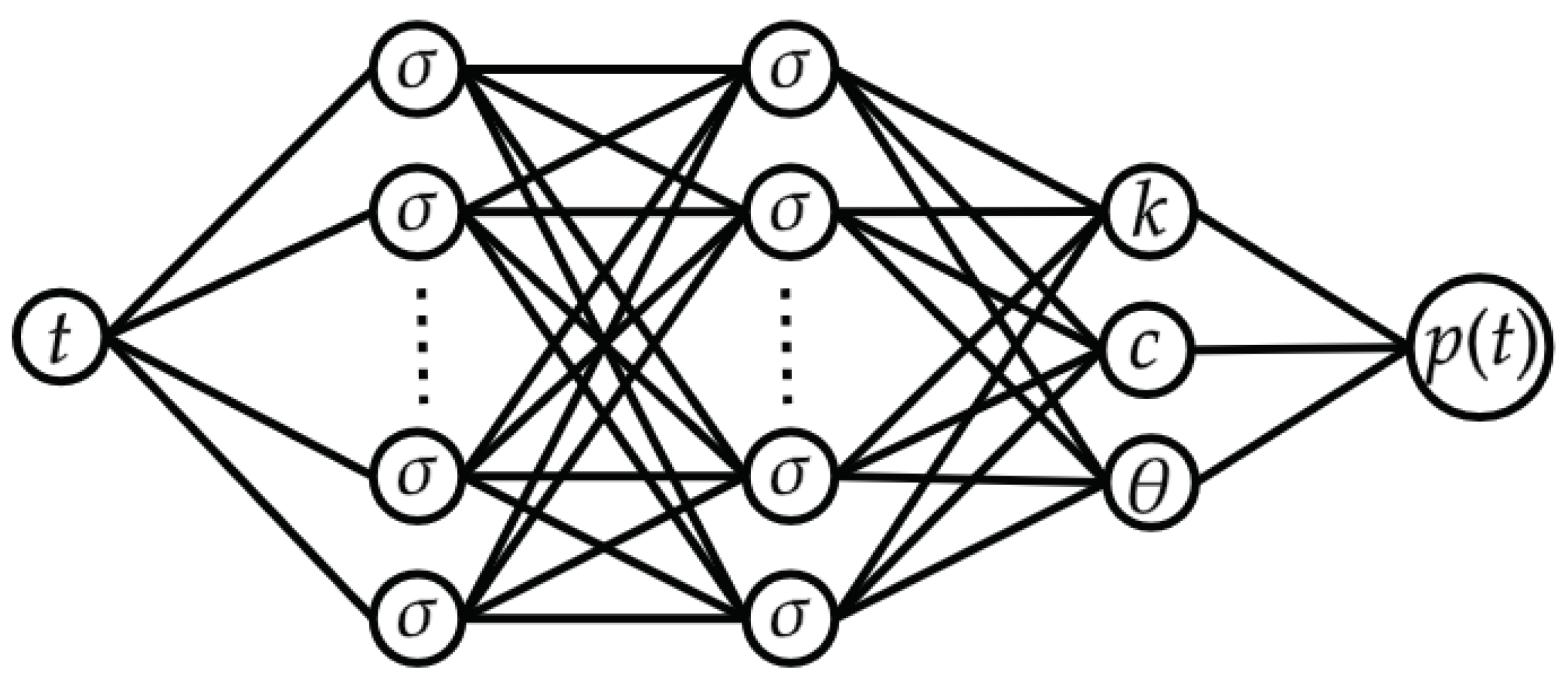
Figure 1 refers to the schematic PINN architecture with the following components:
- Multiple layers, including input, hidden, and output layers. Each layer contains neurons that perform the activation function . Common activation functions include ReLU, sigmoid, and tanh [4].
- The input layer receives input data.
- The output layer produces predictions, the solutions to the problem. This layer might output approximate solutions to the differential equations at different points in time.
- In addition to standard training data, PINNs are trained with physics-informed constraints. These constraints encode the underlying physics of the problem and are used to guide the learning process.
- The loss function measures the error between the predicted solutions and the actual solutions or data. In a PINN, the loss function typically includes terms that penalize deviations from both the observed data and the physics-informed constraints. The network is trained to minimize this combined loss (see Section 2.4).
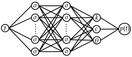
Figure 1.
The schematic PINN architecture for solving differential equations for the Montroll model.
Figure 1.
The schematic PINN architecture for solving differential equations for the Montroll model.
2.4. Loss Function
The PINN was trained by minimizing a physics-informed loss function, which combines the mean squared error between predicted and observed data with terms enforcing the satisfaction of the underlying growth model equations. The loss function was formulated as follows:
where is the data fidelity term and enforces adherence to the growth model equations, and is a regularization parameter [5].
For a set of data points , where denotes input points and corresponds to target values, the data-driven loss might look like the following:
Here, represents the output of the neural network for the model under study for input , and N is the number of data points.
The other term is defined by
Here, is the number of points where the model’s restrictions need to be satisfied, and is the residual of the model at point .
This component ensures that the solution satisfies the underlying physical laws or constraints. It is formulated based on the governing equations or other physics-related constraints.
Choosing an appropriate regularization parameter is crucial for achieving convergence and preventing divergence during training. This selection process often involves experimentation and validation techniques to find the regularization parameter that results in the best generalization performance on unseen data.
The domain of the regularization parameter depends on the specific regularization technique being used. Two common types of regularization are L1 regularization (Lasso) and L2 regularization (Ridge). For both L1 and L2 regularization, regularization typically ranges from 0 to positive infinity [8].
3. Algorithm for Calculating Mean of Residuals
Here, we introduce the algorithm for calculating the mean of residuals for the Verhulst growth model in a PINN framework:
- Initialization:
- Initialize the neural network parameters (weights and biases) randomly or using a predefined initialization scheme.
- Define the training dataset, consisting of input–output pairs representing observations of the population size at different time points from Table 1.
 Table 1. Chinese hamster V79 fibroblast tumor cells [10].
- Forward Pass:
- Perform a forward pass through the neural network to obtain predictions for each input time .
- Compute Residuals:
- Calculate the residuals for each predicted population size , , using the Verhulst model equation.
- Calculate Mean of Residuals:
- Compute the mean of the residuals .
- Update Neural Network Parameters:
- Use an optimization algorithm (in this case, ADAM) [9] to update the neural network parameters to minimize the mean of residuals.
- Repeat:
- Repeat steps 2–5 until convergence criteria are met (e.g., maximum number of iterations reached or convergence of the loss function).
Usually, a first-order differential model requires an initial condition to become a well-posed problem. Here, this condition will be inferred from the experimental data available in Table 1, and then one can use as the initial condition.
4. Results
In this section, we present the results obtained from the application of PINNs for the Verhulst and Montroll growth models to the dataset of tabulated data in Table 1. In this study, we used previously published data from Chinese hamster V79 fibroblast tumor cells [10]. The dataset consists of 45 measurements of volumes ( νm3) over a time period of 60 days.
The main objective of our study was to leverage the combination of supervised learning and physics-based constraints to accurately predict the underlying system behavior and compare the two growth models.
For each method under study, we define the respective loss function depending on the parameters to be determined. Namely, for the Verhulst model,
and for the Montroll model,
As a result of applying the algorithm outlined in Section 3 to each of the functions (6) and (7), we derive the parameters for Table 2 and Table 3 and, consequently, the solutions depicted in the graphs in Figure 2 and Figure 4, respectively. This iterative process allows us to efficiently extract the necessary parameters from the given functions, thus facilitating the generation of the corresponding graphical representations. Through this approach, we visually represent the obtained solutions (in blue) compared to the data provided (in red).
Table 2.
Predicted final parameters for the Verhulst model.
Table 3.
Predicted final parameters for the Montroll model.
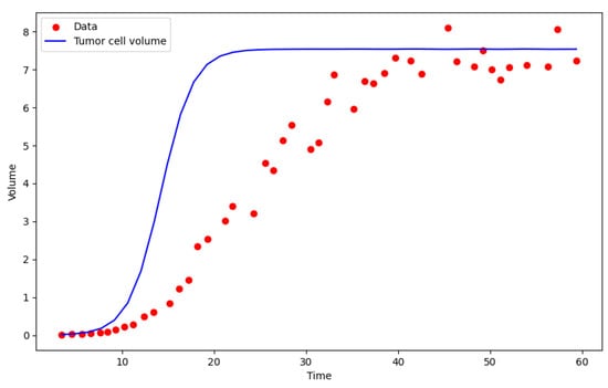
Figure 2.
The PINN solution for the Verhulst model. Volumes ( νm3) over a time period of 60 days.
In Figure 2, we see the graph of the solution predicted by the Verhulst model for the data obtained at the end of a process of 5000 epochs. The evolution of the model’s performance can be seen in Figure 3.

Figure 3.
The history of the total loss function for the Verhulst model.
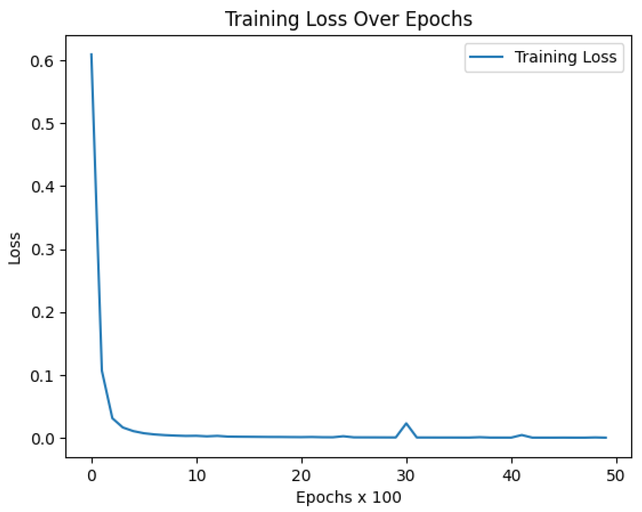
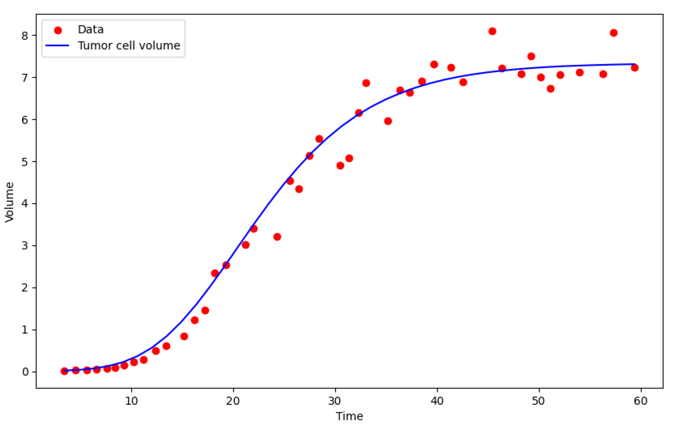
Similarly, in Figure 4, we see the graph of the solution predicted by the Montroll model for the data obtained at the end of the same process of 5000 epochs, while the evolution of the model’s performance can be seen in Figure 5.
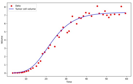
Figure 4.
The PINN solution for the Montroll model. Volumes ( νm3) over a time period of 60 days.
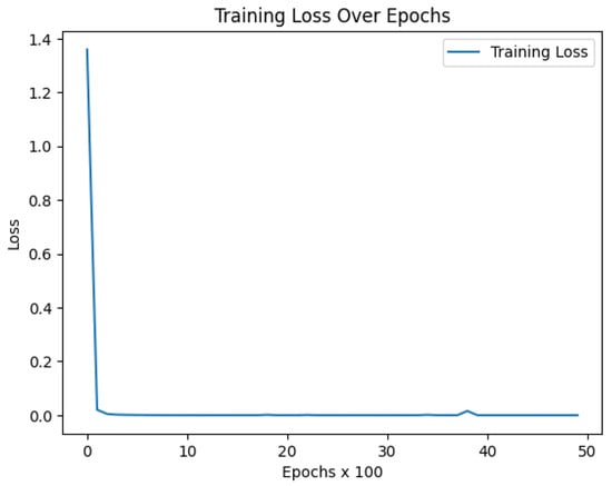
Figure 5.
The history of the total loss function for the Montroll model.
5. Discussion
For both models, we found that the PINN methodology can predict the asymptotic behavior of the saturation of tumor cell volume growth. However, the existence of the parameter of the Montroll model allows a better fit to the data and a better prediction of the location of the inflection point of the growth function graph.
6. Conclusions
This study intended to use Physics-Informed Neural Networks to choose the method that best fits the data, as in a reverse engineering procedure, determining the parameters intrinsic to each method.
The methodology presented for adjusting the growth model can be adopted for any other phenomenon that is intended to be mathematically modeled based on experimental data.
PINNs provide a means of learning robust and accurate models of systems, providing existing domain knowledge about the models that govern the data, even in situations where the equations do not exactly match the data.
Funding
This research was partially sponsored with national funds through the Fundação Nacional para a Ciência e Tecnologia, Portugal-FCT, under project UIDB/04674/2020 (CIMA), available online: https://sciproj.ptcris.pt/157598UID, accessed on 14 March 2024.
Data Availability Statement
Publicly available datasets were analyzed in this study. This data can be found in Ref. [10].
Conflicts of Interest
The author declares no conflicts of interest.
References
- Kamyab, S.; Azimifar, Z.; Sabzi, R.; Fieguth, P. Deep learning methods for inverse problems. PeerJ Comput. Sci. 2022, 8, e951. [Google Scholar] [CrossRef] [PubMed]
- Chen, Q.; Ye, Q.; Zhang, W.; Li, H.; Zheng, X. TGM-Nets: A deep learning framework for enhanced forecasting of tumor growth by integrating imaging and modeling. Eng. Appl. Artif. Intell. 2023, 126, 106867. [Google Scholar] [CrossRef]
- Lorenzo, G.; Ahmed, S.R.; Hormuth, D.; Vaughn, B.; Kalpathy-Cramer, J.; Solorio, L.; Yankeelov, T.; Gomez, H. Patient-specific, mechanistic models of tumor growth incorporating artificial intelligence and big data. arXiv 2023, arXiv:2308.14925v1. [Google Scholar] [CrossRef] [PubMed]
- Raissi, M.; Perdikaris, P.; Karniadakis, G.E. Physics-informed neural networks: A deep learning framework for solving forward and inverse problems involving nonlinear partial differential equations. J. Comput. Phys. 2017, 335, 66–97. [Google Scholar] [CrossRef]
- Sirignano, J.; Spiliopoulos, K. DGM: A deep learning algorithm for solving partial differential equations. J. Comput. Phys. 2018, 375, 1339–1364. [Google Scholar] [CrossRef]
- Bacaër, N. Verhulst and the logistic Equation (1838). In A Short History of Mathematical Population Dynamics; Springer: London, UK, 2011; pp. 35–39. [Google Scholar]
- Goel, N.S.; Maitra, S.C.; Montroll, E.W. On the Volterra and Other Nonlinear Models of Interacting Populations. Rev. Mod. Phys. 1971, 43, 231–276. [Google Scholar] [CrossRef]
- Yang, L.; Zhu, D.; Liu, X.; Cui, P. Robust Feature Selection Method Based on Joint L2,1 Norm Minimization for Sparse Regression. Electronics 2023, 12, 4450. [Google Scholar] [CrossRef]
- Azevedo, B.; Rocha, A.; Pereira, A. Hybrid approaches to optimization and machine learning methods: A systematic literature review. Mach. Learn. 2024. [Google Scholar] [CrossRef]
- Marusić, M.; Bajzer, Z.; Freyer, J.P.; Vuk-Pavlović, S. Analysis of growth of multicellular tumour spheroids by mathematical models. Cell Prolif. 1994, 27, 73–94. [Google Scholar] [CrossRef] [PubMed]


Disclaimer/Publisher’s Note: The statements, opinions and data contained in all publications are solely those of the individual author(s) and contributor(s) and not of MDPI and/or the editor(s). MDPI and/or the editor(s) disclaim responsibility for any injury to people or property resulting from any ideas, methods, instructions or products referred to in the content. |
© 2024 by the author. Licensee MDPI, Basel, Switzerland. This article is an open access article distributed under the terms and conditions of the Creative Commons Attribution (CC BY) license (https://creativecommons.org/licenses/by/4.0/).