Abstract
Legged locomotion is essential for navigating challenging terrains where conventional robotic systems encounter difficulties. This study investigates the sensitivity of the reconfigurable Klann legged mechanism (KLM) to variations in the input geometric parameters, such as joint position location, link lengths, and angles between linkages, on the continuous coupler curve, which represents the output trace of the leg movement.The continuous coupler curve’s sensitivity is explored using global sensitivity analysis based on Sobol’s sensitivity method. Furthermore, a novel reconfigurability strategy is presented for the Klann mechanism, aiming to reduce the number of required actuators and the complexity in control. In simulation, the coupler curves obtained from the reconfigurable KLM are classified as hammering, digging, jam avoidance, and step climbing using machine learning approaches. Experimental validation is presented, discussing an approach to identifying geometric parameters and the resultant coupler curve. Illustrations of the the complete assembly of the reconfigured KLM with the obtained gaits using limited experiments are also highlighted.
Keywords:
reconfigurable robot; Sobol’s method; sensitivity analysis; Klann legged mechanism; geometric parameters MSC:
70B15; 90C31; 93B51
1. Introduction
The utilization of mobile robots in various fields, such as construction, inspection, delivery, security, and monitoring, has seen a significant increase in recent years due to their reliability and efficiency. However, the deployment and application of mobile robots in outdoor environments present significant challenges due to the unstructured and unfamiliar nature of these settings. To address these challenges, research in the field of mobile robotics has focused on the development of legged locomotion drive mechanisms. Legged mobile robots possess distinct advantages over wheeled mobile robots, particularly in their ability to traverse a wide range of terrains and adapt to overcome obstacles in unpredictable environments while maintaining stability during terrain changes. This makes legged mobile robots well suited for deployment in outdoor environments and has led to increased interest in the development and deployment of legged mobile robots.
Modern legged robots are classified based on the number of legs and degrees of freedom, which determine their gait and usage scenarios. Mono-pedal robots, as discussed in [1], are restricted to saltatorial locomotion and have limited mobility. On the other hand, eight-legged robots have the potential to perform a wide range of gaits, depending on their design. Bi-pedal robots present a challenge in design and sensory input due to their requirement for maintaining stability during forward and backward motion as well as during steady state [2,3]. Quadruped robots offer stability and greater freedom for reconfigurability and multiple gait generation for different scenarios [4] but require computational resources and complex control systems to adjust to real-time sensory feedback as demonstrated in [5], which proposes a metamorphic quadruped robot using an 8-bar linkage mechanism to mimic the gait patterns of arthropods, mammals, and insects. To achieve further stability, researchers have proposed hexapod robots that imitate biological gaits [6,7]. Algorithms for gait generation for hexapods and stable locomotion have also been proposed, such as an adaptive 3D, double-layer CPG network for basic locomotion patterns, and reinforcement learning-based algorithms to regulate leg behavior [8,9]. To simplify legged robot control systems while preserving functionality, planar linkage-based mechanisms, such as the Klann Legged Mechanism (KLM) and Theo Jansen Legged Mechanism (TJLM) proposed in [10,11], offer scalability, deterministic foot trajectory, and power efficiency. These one-degree-of-freedom solutions require fewer actuators, allowing multiple legs to be controlled with just one motor, making them highly efficient for legged robots. The KLM, known for its multi-terrain capability, reduced payload, and computation load, has been utilized in [12] for a robot with dual functionality on land and water. Despite these advancements, the design of these robots which requires multiple actuators for each leg and a complex control system for cohesive and sensible locomotion, continues to impose a significant computational burden on the robot.
Reconfigurable robotics has made notable progress; its taxonomy is detailed by Tan et al. (2020) [13], and Hayat et al. (2022) [14] presented the heuristic approach to design reconfigurable robots. Reconfigurable legs in robotics have garnered attention for their capacity to improve adaptability and performance. In engineering and design, the synthesis of mechanisms often involves understanding the requirements of a system, identifying the constraints, and then designing a set of interconnected parts that can fulfill the intended purpose. Notably, Nansai et al. (2015) introduced a novel Theo Jansen linkage capable of producing diverse gait cycles, demonstrating its potential for innovative applications [15]. Sun and Zhao (2019) proposed a strategy for reconfigurable robots using shape morphing joints, enabling multiple trajectories without altering the mechanical design [16]. Kim et al. (2017) developed Snapbot, a reconfigurable legged robot with detachable magnetic legs, showcasing various styles of legged locomotion [17]. Guan et al. (2022) showcased a reconfigurable legged robot with a flexible waist, exhibiting enhanced motion performance and adaptability, while Tang et al. (2022) introduced Origaker, a multi-mimicry quadruped robot with a metamorphic mechanism, enabling transformations between reptile-, arthropod-, and mammal-like modes, emphasizing the versatility and potential of reconfigurable legs in robotics [18,19]. The reconfigure leg was studied in [20] regarding the exact link lengths and angle changes required for generating the five types of gait patterns. While achieving reconfigurability, the latter method involves seven actuators in each leg, adding complexity to the control system and design. The influence of link lengths and input angles on Klann mechanism gait patterns is only studied by varying one parameter at a time (OAT), and also in different range [21]. The sensitivity analysis with uniform range variation in the geometric parameters and capturing global sensitivity is essential.
Sensitivity analysis, particularly global sensitivity analysis (GSA), plays a crucial role in understanding and quantifying the impact of input variables on the output of complex mathematical models. Sobol proposed global sensitivity indices that efficiently assess the influence of individual or groups of variables using Monte Carlo methods [22]. It was extended in [23] by introducing new importance measures based on failure probability, enhancing the understanding of reliability-related sensitivity. In the realm of engineering applications, Nguyen et al. (2020) applied Sobol’s GSA to assess the in-plane elastic buckling of steel arches, considering random input parameters [24]. A sampling-based sensitivity analysis method for engineering products with uncertain input variables, reducing computational complexity and increasing efficiency, is discussed in [25]. This method enables assessing input factors impact on model responses without predefined probability distributions, enhancing sensitivity analysis applicability in complex engineering scenarios.
From the above discussion, the objectives and contributions of this work are listed below:
- Sensitivity analysis: Conduct a detailed analysis of the sensitivity of the reconfigurable Klann legged mechanism to variations in the geometric parameters using Sobol’s method. Towards this end, the kinematics of the KLM is also presented.
- Reconfiguration strategy: Studying the sensitivity of the Klann mechanism model makes it possible to reconfigure using a minimal number of actuators, i.e, using only two rotary actuators, five types of gait are achieved.
- Gait classification: Implement machine learning approaches, including K Nearest Neighbors (KNNs), Decision Tree, and Random Forest algorithms, for the classification of generated gaits based on altered positions of the lower rocker and the angle of the end effector.
- Experimental validation: Validate the proposed reconfigurable Klann legged mechanism through experimental assembly, ensuring practical applicability and performance verification.
The paper is structured into six sections. The introduction, i.e., Section 1, underscores the importance of reconfigurability in robotics, focusing on the Klann Legged Mechanism’s adaptability. Section 2 highlights the motion study and gait trajectories. Section 3 explores the reconfigurability principles and conducts a detailed sensitivity analysis. Section 4 discusses the gaits classification and the aspects towards achieving reconfigurability in KLM, whereas Section 5 presents the testbed with a single leg of KLM, the identification of geometric parameters using computer vision, and CAD assembly. The paper concludes by summarizing the key findings in Section 6.
2. Kinematics and Gaits of KLM
In this section, the kinematics that deals with studying the motion of the object without regarding the forces that causes it is presented for the Klann Legged Mechanism. Moreover, the output, in the form of a coupler curve or gait trajectory nature, is also highlighted.
2.1. Position Analysis
The KLM works by converting the rotational movement of the input crank into a translational movement of the end effector, which in this case is the leg assembly. As the input crank rotates, it causes the various six-bar linkages in the linkage to move in a coordinated manner, resulting in the end effector (the leg assembly) moving in a walking motion. The Klann mechanism can be considered to be made of two four-bar mechanisms as shown in Figure 1. The first four-bar mechanism is OCDA with OC as the input crank, whereas the second is made by joining the AL as the imaginary link and forming as BELA. The trajectory of the foot is constrained by the properties of these two four-bar mechanisms. Considering the four-bar mechanism as OCDA:
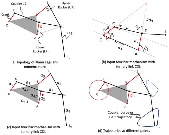
Figure 1.
Standard topology and nomenclature of the Klann linkages or KLM.
By utilizing the four quadrant atan2 operator, the four-bar mechanism can be assembled in two modes that correspond to different signs before the arccosine in the previous equation. Once the values of and (Figure 1b) are known, it is possible to uniquely define the positions of points C, D, and L with:
where
and are the constants introduced as shown in Figure 1. With the points L and B being known, the position of Point E can be found using the bilateration problem reported in [26,27]. Bilateration is a mathematical technique used to determine the position of an object using the distance measurements from that object to two or more known locations, called anchors or reference points. In two-dimensional bilateration, the location is determined by finding the intersection point of two or more circles, each centered at an anchor point with a radius equal to the distance from the object to that anchor. Geometrically, for two vectors, represent the intersection of two circles, one with the center at L and another at B with a radius as the link lengths indicated in Figure 1:
where and with
There exist two possible positions for point E, leading to a total of four solutions for Klann’s linkage in terms of its forward kinematics. By differentiating the above equation, the velocity and acceleration of the gait or link positions can be determined during the rotation of the crank.
2.2. Continuous and Discontinuous Gaits
The position kinematics of the KLM highlighted in Equations (4) and (5) are non-linear in nature. A small change in the geometric parameters can lead to significant changes in the system behavior. Figure 2a shows the continuous curve traced by the leg movement. The cyclic rotation of the crank is possible for the given geometric parameters. In the continuous gait, the legs move in a coordinated manner, producing regular and predictable stepping patterns. Figure 2c highlights the velocity and acceleration plots, indicating that the values are within the design limit and the curves are continuous. The geometric configuration obtained by changing the position of the hinged joint result in a discontinuous gait as shown in Figure 2b. The corresponding velocity and acceleration plot are shown in Figure 2d. The discontinuous gait results in more abrupt changes in acceleration. The discontinuous gait also impacts stability. It may provide advantages in specific applications, where intermittent motion is desirable. The sensitivity of the geometric parameters for the KLM is discussed in the next section.
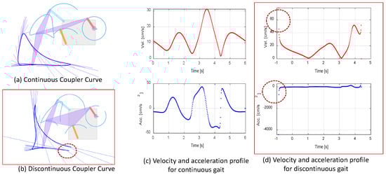
Figure 2.
Continuous and discontinuous gait patterns obtained with reconfigurable KLM.
3. Sensitivity Analysis for Reconfigurable KLM
This section emphasizes the role of reconfigurability in KLM. It provides a detailed sensitivity analysis and its computation using the Monte Carlo approach, quantifying the input variations’ impact on the output. The study focuses on evaluating the geometric parameters sensitivity of the Klann Legged Mechanism (KLM) as illustrated in Figure 3. It also outlines and illustrates the various modes of reconfigurability in the KLM by an arrow on the kinematic structure, indicating the changes in the geometric parameters.
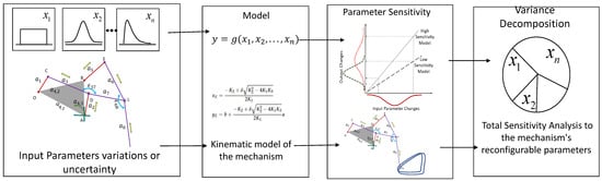
Figure 3.
Schematic diagram of the sensitivity analysis.
3.1. Parametric Sensitivity Analysis
Sensitivity analysis based on variance capitalizes on the inherent uncertainty in the input parameters. This method quantifies the importance of each factor through the calculation of a sensitivity index, whereas the partial derivative or the Jacobian methods analyze individual parameter changes one at a time by explicitly examining the influence of each parameter on the model’s output.
Given a non-linear model, , where represents the input parameters and y is the scalar output, the contribution of uncertainty (represented by the probability density function of ) to y can be quantified through
where Var denotes the variance, and is the conditional expectation of y given . This measure is referred to as the first-order sensitivity index (FSI). While it shares similarities with the partial derivative concept (), which represents local sensitivity, it does not capture the combined effect of interactions between two parameters on the output variance.
Sobol’s method, on the other hand, evaluates the contribution of each input parameter to the total output variance. It is a variance-based sensitivity analysis. For total sensitivity analysis (TSI), the variance-based sensitivity measure, which was first presented in [28], is commonly used. This method measures the primary impact of a specified parameter along with any related influences. The overall influence of parameter on the output, for example, is given by
where is the total sensitivity index (TSI) for parameter . This is based on the consideration of three input parameters, , , and . The first-order sensitivity (FoS) of parameter is represented by the term . For briefness, an extensive description of Sobol’s technique is given in the following section.
3.2. Computation of Total Sensitivity Index Using Monte Carlo Technique
The total variance and partial variances can be computed using the Monte Carlo-based technique for integration, which makes Sobol’s method relatively easy to implement. For a given sample size N, the estimates are:
where is a sampled point in the input parameters, and N is the sample size of quasi-random data points inside the hypercube. The Monte Carlo estimate of the output variance is represented as:
The total sensitivity indices were calculated using the two subsets of the variables, namely, and , where is a complimentary vector of input variables except . The sensitivity of the complimentary vector of variables can be calculated using just one integral expressed in discrete form with N-trials:
Hence, the GSI for is . As presented in Saltelli and Sobol [29], the set of input parameters can be grouped into two sub variables such that one is and the other group is complementary to as . Simply, the set of variables where s is a single variable out of the total n numbers and the complimentary to the variable is the vector of variables , which excludes . The Monte Carlo method was constructed using two sets of independent random numbers generated for each element of input vector ( has n-elements). Let and be the two sets of uniformly distributed random numbers of size (N is the number of random sample points generated, and n is the numbers of parameters for which sensitivity analysis is performed), with and . In total, three computations of the model , and are required with N-trials to obtain the Monte Carlo estimates as:
The number of trials or model calls approximately required are [30] to estimate the Sobol’s index of one input with an uncertainty of 10%. From the above expressions, it is easier to calculate the first-order sensitivity index of parameter as , and Total Sensitivity Index (TSI) as . The measure is referred to as “first-order sensitivity” by Sobol (1993) and it measures the only main contribution of the input on the output variance while neglecting the other interactions. The TSI are greater than the first-order sensitivity indices (FSI). The steps to implement the Monte Carlo scheme for the sensitivity analysis are given in Algorithm 1. Appendix A also discuss the sensitivity of the Ishigami function estimated using the algorithm listed, and the codes are also shared. In the next section, the sensitivity of KLM with its dimensions are highlighted.
| Algorithm 1 Algorithm to find the Total Sensitivity Index (TSI) of parameters. |
|
3.3. Illustration with the Reconfigurable KLM
Klann’s linkage offers a variety of walking gaits due to its six links’ topology. This reconfigurability feature for the KLM can be achieved mainly with the three modes listed below:
- Changing link lengths: This straightforward approach involves adjusting the lengths of the links, except the crank and end effector, using linear actuators. This method was studied in previous works and resulted in six useful gait patterns.
- Changing coupler link angles: The coupler is a key component that connects the input and output links. Adjusting its angle alters the foot’s trajectory.
- Changing grounded joints hinge positions: This novel approach proposes changing the position of the revolute joint connecting the crank, lower, and upper rocker to the fixed base, affecting the coupler joint’s range of motion and the end effector’s overall movement.
The dimensions selected in centimeters as shown in Figure 4 Left, are crank () = 11, lower rocker () = 13, upper rocker () = 17, coupler (a3) = 28, and () = 23, leg () = 26, and end effector () = 30. The angle deviation between coupler () is () and is 170 degrees. For the standard gait, the angle between the end effector and leg () is 160 degrees. The effect of change in each parameter one at a time (OAT) on the output, i.e., the trace of the end effector of the KLM, is discussed below.
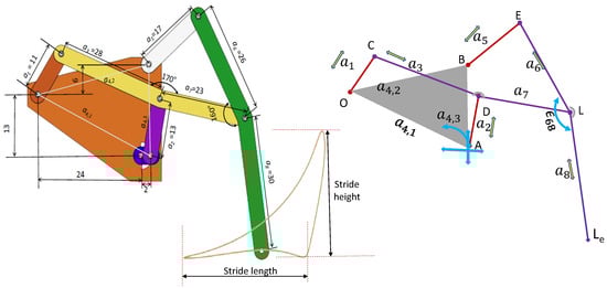
Figure 4.
Reconfiguring the Klann Legged Mechanism (KLM).
The changes in the geometric parameter, namely, are as follows.
- Crank length (): The standard crank length considered is 11 cm, and it is varied from 3 to 14 cm. The range in which the crank length can be varied is ideally from to 14, so with an interval of 14 cm. The variation observed in the gait trajectory is that of scale, where both the stride length and height are increasing with the increase in the crank length as shown in Figure 5a.
- Lower rocker length (): The standard rocker length is considered 13 cm, and it is varied from 12 to 23 cm with a step of 1 cm as shown in Figure 5b. An increase in the length of leads to an increase in the height and a decrease in stride and vice versa. The step heights remain approximately the same. The slope of the return stroke also changes considerably.
- Upper rocker length (): The standard upper rocker length is kept as 17, and the length is varied from 14 to 35 cm. The decrease in length below 14 results in a discontinuous gait while the increase in length is allowed to vary. Figure 5c shows the variation due to the change in the length of .
- Coupler length (): The effect of the change in the length parameter of CD and DL or effectively CL is that the stride height effectively remains the same, whereas the stride length increases. The variation is also allowed and checked with the increase and decrease in the length by 10%.
- Base length (): The standard length of is considered 29. An increase in its dimension leads to an elongation of the stride length and a reduction in step height and vice versa. This suggests that the changes approximately maintain the area under the curve by the generated gaits. The range to vary this length is also lesser, i.e., −28 to 30.4 as shown in Figure 5e.
- Leg angle (): The angle in between for the leg, i.e., angle ELM, is varied and the effect is a change in the orientation of the gait, which as a result leads to a decrease in the effective length of the contact point with the ground. The standard value is kept as 160 degrees, and it is varied between 140 and 170 degrees.
The approach of changing the geometric parameters one at a time to obtain different gait patterns, such as hammering, digging, jam avoidance, step climbing or others, are studied in [31] by varying the geometric parameters one at a time (OAT). Also, varying the coupler angle OAT is reported in [16]. Moreover, no comments were made on the variation range of these individual parameters. These were briefly discussed in the above paragraph. Moreover, the range of varying these parameters is different; hence, the sense of the total and normalized effects is not reflected.
The total sensitivity of the geometric parameters were calculated using the following steps:
- Select the number of input geometric parameters for sensitivity analysis.
- Define the range for perturbation values associated with these parameters. Gaussian distribution was utilized to allocate perturbations to each parameter. Intervals were specified as () and () for length parameters and angular parameters.
- Sensitivity analyses were conducted for the selected parameters, focusing on their impact on the robot’s outputs, specifically its position and orientation.
- The sensitivity indices for these parameters were subsequently determined using Algorithm 1.
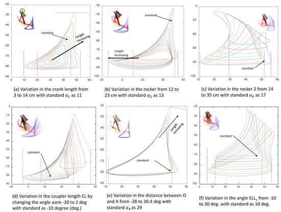
Figure 5.
Illustration of the sensitivity of parameters change one at a time (OAT) on the gait trajectory.
The bar chart in Figure 6a,b presents the Total Sensitivity Index of the geometric parameters, namely and of the reconfigurable KLM on the X and Y coordinates of the geometric center of the gaits curve. In the context of sensitivity analysis using the Sobol method, the simulation involves changing the length parameters by 1% and angle variations ( and ) by 1 degree. The Monte Carlo approach was used as discussed in Algorithm 1, while the simulation was run 10,000 times to estimate the total sensitivity indices.
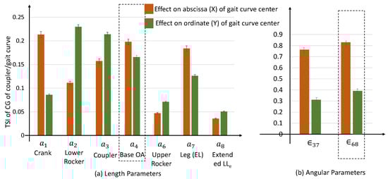
Figure 6.
Total Sensitivity Index (TSI) for the length and angular parameters using Sobol’s method.
The analysis of the sensitivity indices reveals that the parameter and angle exhibit notable sensitivity in both the abcissa and ordinate, i.e., x and y coordinates of the gait curve generated. This indicates that changing or reconfiguring parameters and using a suitable design approach will lead to the required gaits, which have the feature of different stride heights and widths as indicated in Figure 7. The Sobol total sensitivity indices for these parameters indicate a significant influence on the output of the reconfigurable KLM. This suggests that variations in the length parameter and angle contribute significantly and can be varied to obtain the required gaits just by varying these two with particular settings. The analysis is used to vary these parameters and design the reconfiguration in KLM using only these two parameters in the next sections, satisfying the condition of continuous gait as well. Algorithm 1 as presented is generic and can be extended to analyze any non-linear and differentiable functions.
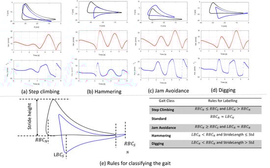
Figure 7.
Different gaits generated along with its velocity and acceleration profile. The rule for classification of the gaits under step climbing, jam avoidance, hammering, and digging w.r.t. the standard gait.
3.4. Discussion on Aspects of Sobol’s Method
Sobol’s method presents several advantages when employed for sensitivity analysis in the context of studying non-linear kinematic functions with an example of the Klann Legged Mechanism (KLM) in this work. One notable strength lies in its ability to provide a global perspective by considering the entire variation range for each input parameter, capturing intricate non-linear interactions. This comprehensive approach offers a more holistic understanding of how parameters collectively influence the output. It is especially crucial for a complex system like the KLM with diversity in the nature geometric parameters, i.e., linear and angular and also in the magnitude in which each parameter can vary. This is illustrated and studied in the above section, i.e., Section 3.3, and the interpretation results in selecting the geometric parameters for the reconfiguration purpose. Additionally, Sobol’s method quantifies sensitivity through sensitivity indices (SIs), allowing for the prioritization of parameters and identification of key drivers affecting the output variability. Its flexibility extends to accommodating the KLM non-linearities and handling a multitude of input parameters efficiently, particularly when implemented through Monte Carlo simulations.
Despite these merits, Sobol’s method has its limitations. Computational costs, while relatively efficient, can still pose challenges for models with more parameters or more intricate interactions. The black-box nature of Sobol’s method, providing numerical results without explicit functional relationships, may be a drawback. Assumptions of parameter independence may not always align with real-world scenarios, potentially leading to some inaccuracy in the sensitivity estimates. Moreover, interpreting the relative importance of parameters can be challenging, especially in the presence of complex interactions and multiple output variables. Overall, Sobol’s method offers a powerful tool for comprehensive sensitivity analysis of nonlinear functions. However, it is important to be aware of its scope and consider alternative methods if necessary.
4. Classification of Gaits Using Machine Learning Approaches
The classification of gaits in a reconfigurable mechanism is essential. The use of a machine learning prediction [32] model further enhances this classification process. Predicting the stride length and height are crucial parameters for identifying the resulting gait class among the different categories.This section emphasizes ML approaches towards classifying gaits.
Figure 7a–d visually categorize gaits into distinct classes, such as standard, step climbing, hammering, jam avoidance, and digging along with its position, velocity and acceleration diagram. To train the prediction model, an image data set consisting of over 1100 images (the data set along with code can be found in the link: https://drive.google.com/drive/folders/1U8lTBJXoNhxRnVc7QtoswXQwm1mRSVy4?usp=sharing, accessed on 25 January 2024) was generated by randomly varying the position of the lower rocker and the angle of the end effector. Since almost all gaits generated using this method fall under one of the five categories, albeit with unique stride parameters, a rule base was defined for labeling the images into classes. Each image is saved with a file name that includes the percentage change in the X and Y axes of the lower rocker, the stride length and stride height, as well as the class to which the gait belongs to. These parameters are parsed for each individual image, and a data frame is created for training. Various machine learning approaches for classification exist, such as Logistic Regression, Naive Bayes, Support Vector Mechanism, K Nearest Neighbors (KNNs), Decision Tree (DT), Random Forest (RF), etc. Since multiple classes are involved, in this work we have used KNN, Decision Tree, and Random Forest to train and evaluate the data as shown in the flow diagram in Figure 8. The data set was divided into training and testing sets, with 80% of the data used for training and the remaining 20% for testing. Standard transformation was applied to the features to ensure minimal bias, and then they were fed into the classifier.
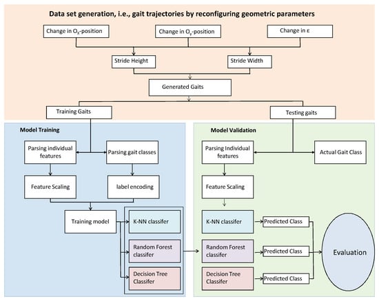
Figure 8.
Flow diagram for the classification schemes used.
KNN classification, with a total accuracy of 94%, makes the best use of the feature space and is a relatively simple machine learning algorithm. The number of nearest neighbors to be considered during classification was set to 4, as it provided a balance between the testing and training set accuracy. The model was also trained using a DT classifier, considering the hard limits during labeling based on stride parameters for the digging and hammering gait patterns. The accuracy by using this classifier was 89%, and the evaluation metrics are laid out in Table 1. Furthermore, a RF classifier was used, setting the number of trees/estimators in the forest as 100, which gave us the best results as of yet with an accuracy score of 95%. The evaluation parameters related to the random forest classifier are shown in Table 1.

Table 1.
Evaluation metrics for the classifiers towards the gaits generated. KNN (K-Nearest Neighbors), DT (Decision Tree), and RF (Random Forest) refer to three distinct classification algorithms.
The results demonstrate that both the KNN and Random Forest classifiers achieved comparable levels of accuracy and F1-Score in classifying gaits. However, in the case of an unbalanced data set, the KNN classifier outperformed the Random Forest classifier in terms of the overall F1-score. It is recommended to use the KNN classifier for classifying gaits in our proposed variation for reconfigurability, as it provides valuable insights into the types of gaits that can be generated and their corresponding stride length and height by modifying three parameters. The only limitation is that it requires users to know the changes they are making and input them to the model. However, this limitation can be addressed by using a computer vision algorithm to analyze the link parameters also discussed in the next section.
5. Experimental Studies with the Proposed Design of Reconfigurable KLM
In this section, the proposed design of the reconfigurable KLM based on changing the parameters and as shown in Figure 4 and its global sensitivity analysis indicated in Figure 6 is designed. It is also tested for the gait generation by varying the parameters and classifying the gaits based on Section 2.2. The objective of the proposed design is the use of minimal actuators that are rotary against the multiple linear actuators proposed earlier in [20]. It is important to note that, inherently, the KLM is designed with single degrees of freedom (DoFs) in actuator space, i.e., only one motor is sufficient to generate the gait. Here, for reconfigurability, additional actuators are added but are assumed to be in a locked state for a given configuration, and only the crank is rotated.
5.1. Single Reconfigurable KLM Testbed
The single-leg model of the Klann linkage with the provision to change the hinge location and the leg joint angle is shown in Figure 9a. The testbed is constructed using 5 mm thick multi-wood to showcase various gait patterns. Figure 9b shows that by adding the additional link with a given constraint to the joint position J3 (Figure 9a), it moves in a circle.Figure 9b also indicates that the continuous curves are obtained; even the joint positions subject to Grashof’s Law for planar linkages are also satisfied.The aim is to utilize this model for tracing different gait patterns resulted from changing the two parameters. We proposed the computer vision technique to estimate the link lengths as well, in order to predict the gaits generated using the classification model (Section 4) with the kinematic model detailed in Section 2. The single-leg model serves as a practical tool for testing and obtaining results, affirming the proposed approach’s validity.
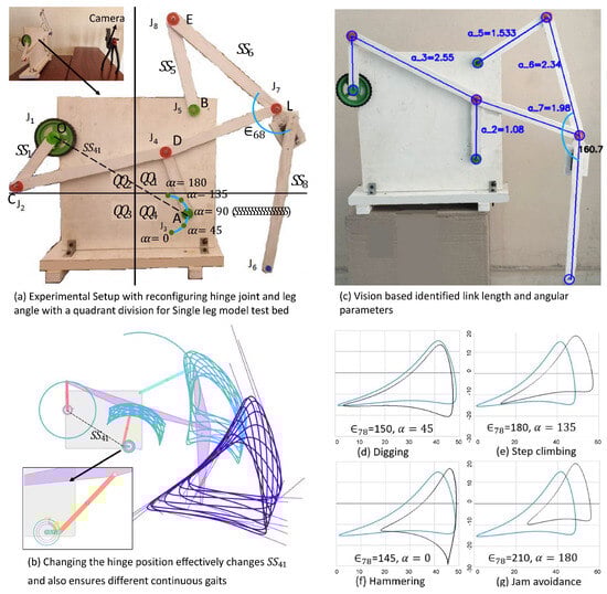
Figure 9.
(a) Experimental setup of a single reconfigurable KLM, (b) model replicated with overlaid gaits for illustration using [33,34] (c) geometric parameters estimation using machine vision, and (d–g) different gaits obtained.
5.2. Identification of the Geometric Parameters Using Computer Vision
In linkage mechanisms, the ratio between link lengths significantly influences the produced gaits. Adjusting a single link’s length, either scaling up or down, maintains the gait shape, with noticeable changes confined to the stride parameters. The identification of the geometric parameters was also proposed in order to estimate them using computer vision. The approach of using computer vision to estimate the geometric parameters of industrial robot is studied in [35] using the circle point methods detailed in [36,37]. In this paper, we used markers to simplify the estimation of the joint location and then calculated the pixel length, which can be scaled to the actual length.
The computer vision algorithm employs a masking-based detection approach to identify joint positions, link lengths, and angles in a robotic mechanism. The steps involve, namely, the following.
- Image preprocessing: converts the image to grayscale, captured using the camera as shown in the experimental setup in Figure 9a.
- Joint identification: applying masking to identify joints based on their color. Red Mask with (a) circle in the quadrant ( or ) is Joint 2 (j2), (b) circle in the quadrant ( or ) with the least X-coordinate is Joint 4 (J4), (c) circle in the quadrant () with the least Y-coordinate is Joint 8 (J8), while the remaining one is Joint 7 as in Figure 9b. Using a green mask, (a) if the circle is in quadrant (), then it is Joint 5; (b) if the circle is in quadrant (), it is Joint 1 (J1), and if the circle is in quadrant (), then it is Joint 3 (J3). The gait trace, i.e., the end of the leg movement, is traced using the blue mask. Following joint identification, the algorithm calculates the Euclidean distances between points and normalizes them based on the crank length ratio. The experiment, conducted with a physical model by varying the crank rotation angles, hinge position of joint J3 and variations, yields the results presented in Table 2. The code for machine vision estimation is also shared in the online folder with the link (Link for the codes and data set used: https://drive.google.com/drive/folders/1U8lTBJXoNhxRnVc7QtoswXQwm1mRSVy4?usp=sharing, accessed on 25 January 2024).
Table 2. Identified value of pixel ratio of link lengths () with respect to crank length () using computer vision. The average ratio is an indicator of the values identified by changing the crank positions.
The actual ratio in Table 2 refers to the calculated ratio between each of the mentioned link lengths with respect to the length of the crank. The average ratio of samples is measured by taking the mean of the predicted ratios predicted by the algorithm for a sample size of 100. Using these measures, the standard deviation for each link length is also estimated. From the results, we can observe that the standard deviation is low, and the algorithm is also predicting the angle and link lengths as shown in Figure 9 with acceptable accuracy. The gaits generated with the values indicated for the pose of the lower rocker are depicted in Figure 9d–g as digging, step climbing, hammering, and jam avoidance, respectively.
5.3. CAD Assembly and Scaled Reconfigurable KLM
Figure 10a,b show a reconfigurable single-leg model and a full-body CAD model, respectively. This model features three gears on each side, the center gear for transmission and the side gears for driving. Notably, the driver gear boasts increased thickness to handle greater force than the driven gears. For achieving a reconfigurable KLM with minimal actuation for versatile terrain maneuverability, we propose a design that modifies the position of the lower rocker. As illustrated in Figure 10a, the lower rocker’s position follows a circular locus with a radius equal to 15% of the distance between the lower rocker and the crank. This design is facilitated by a servo-driven mechanism with a 2 cm radius connected to the lower rocker. Expanding reconfigurability, a servo mount on the upper part of the end leg adjusts the leg’s angle as seen in Figure 10a. This servo connects to the lower part of the end leg via a servo hub. The entire mechanism is driven by a motor connected to a shaft, detailed in Figure 10a. This design empowers the mechanism to adapt to diverse terrains by changing the leg’s position and angle.
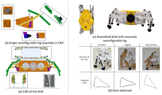
Figure 10.
Assembly of the proof of concept of the reconfigurable KLM in CAD and the experimental setup.
Moving from the CAD model to practical implementation, a reconfigurable KLM assembly scaled at 1/10 of the model shown in Figure 9 was assembled as shown in Figure 10c. Due to size limitations, manual reconfigurable legs were designed to accommodate step climbing, digging, and basic mobility. The angle between the coupler and end effector was adjusted for different locomotion types. Employing computer vision with a blue marker on the leg’s shoe facilitated tracking the end-effector gait. Results from the experiments on this robot match those from the single-leg model, confirming the efficacy and reliability of our strategy as depicted in Figure 10d.
6. Conclusions
The study presented a comprehensive investigation of the reconfigurable Klann Legged Mechanism (KLM) with a focus on its sensitivity of geometric parameters and the classification of gaits using machine learning approaches. This work proposed the reconfiguration of KLM to ahcive five gaits by using only two rotary actuators against five and more linear actuators proposed in literature. The sensitivity analysis revealed that the Klann mechanism is sensitive to changes in and apart from other parameters, and hence is used as a basis to design the reconfigurable KLM by changing them. Overall, Sobol’s method offers a powerful tool for comprehensive sensitivity analysis but it is important to be aware of its limitations highlighted in the paper. The machine learning-based gait classification approach classified four distinct gaits, hammering, digging, jam avoidance, and step climbing, with an accuracy of over 90%, though it is recommended to use KNN for the classification.
The experimental results demonstrated the feasibility of the proposed reconfigurable KLM design and the effectiveness of the gait classification approach. The single-leg testbed with the provision to change the hinge location, i.e., effectively changing length of and the leg joint angle, i.e., was constructed to showcase various gait patterns. The computer vision technique was used to estimate the link lengths and predict the gaits generated using the classification model. Overall, the study provides valuable insights into the global sensitivity analysis and reconfigurability of the Klann Legged Mechanism. The machine learning-based gait classification approach and the experimental results demonstrate the potential of the KLM for practical applications in robotics. Future work involves the assembly of a full-scale model and control approaches for reconfiguration.
Author Contributions
Conceptualization, G.R., D.V.K., A.A.H., R.K.M., M.R.E. and S.N.; methodology, A.A.H., D.V.K., G.R. and S.N.; software, D.V.K., A.A.H. and G.R.; validation, A.A.H. and G.R.; formal analysis, A.A.H., D.V.K., G.R. and S.N.; supervision, R.K.M. and M.R.E. All authors have read and agreed to the published version of the manuscript.
Funding
This research is supported by the National Robotics Programme under its National Robotics Programme (NRP) BAU, Ermine III: Deployable Reconfigurable Robots, Award No. M22NBK0054 and also supported by A*STAR under its “RIE2025 IAF-PP Advanced ROS2-native Platform Technologies for Cross sectorial Robotics Adoption (M21K1a0104)” programme. We wish to acknowledge the support of the SUTD DesignZ Center.
Institutional Review Board Statement
Not applicable.
Informed Consent Statement
Not applicable.
Data Availability Statement
The data presented in this study are available on request from the corresponding author (email: aamir_hayat[at]rediffmail.com). For the codes and data set used: https://drive.google.com/drive/folders/1U8lTBJXoNhxRnVc7QtoswXQwm1mRSVy4?usp=sharing, accessed on 25 January 2024).
Conflicts of Interest
The authors declare no conflicts of interest.
Correction Statement
This article has been republished with a minor correction to the Funding statement. This change does not affect the scientific content of the article.
Appendix A
The Ishigami function is often used as a benchmark problem in sensitivity analysis and uncertainty quantification studies. It is a mathematical function that demonstrates non-linearity and strong interaction effects among its input parameters. The function is defined as . The Ishigami function is particularly interesting for sensitivity analysis because of its nonlinear and non-monotonic behavior, making it a suitable test case for evaluating different sensitivity analysis methods. For further insight, readers are encouraged to refer to the explanation in the online source [38]. The sensitivity analysis calculated based on the algorithm listed in this paper is shown in Figure A1 below.
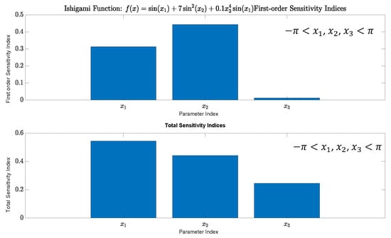
Figure A1.
Ishigami function sensitivity analysis.
References
- Yim, J.K.; Fearing, R.S. Precision jumping limits from flight-phase control in Salto-1P. In Proceedings of the 2018 IEEE/RSJ International Conference on Intelligent Robots and Systems (IROS), Madrid, Spain, 1–5 October 2018; pp. 2229–2236. [Google Scholar]
- Buss, B.G.; Ramezani, A.; Akbari Hamed, K.; Griffin, B.A.; Galloway, K.S.; Grizzle, J.W. Preliminary walking experiments with underactuated 3D bipedal robot MARLO. In Proceedings of the 2014 IEEE/RSJ International Conference on Intelligent Robots and Systems, Chicago, IL, USA, 14–18 September 2014; pp. 2529–2536. [Google Scholar]
- Ramezani, A.; Hurst, J.W.; Akbari Hamed, K.; Grizzle, J.W. Performance Analysis and Feedback Control of ATRIAS, A Three-Dimensional Bipedal Robot. J. Dyn. Syst. Meas. Control 2013, 136, 021012. [Google Scholar] [CrossRef]
- Sun, T.; Xiong, X.; Dai, Z.; Manoonpong, P. Small-sized reconfigurable quadruped robot with multiple sensory feedback for studying adaptive and versatile behaviors. Front. Neurorobotics 2020, 14, 14. [Google Scholar] [CrossRef] [PubMed]
- Tang, Z.; Qi, P.; Dai, J. Mechanism design of a biomimetic quadruped robot. Ind. Robot. Int. J. 2017, 44, 512–520. [Google Scholar] [CrossRef]
- Delcomyn, F.; Nelson, M.E. Architectures for a biomimetic hexapod robot. Robot. Auton. Syst. 2000, 30, 5–15. [Google Scholar] [CrossRef]
- Agheli, M.; Qu, L.; Nestinger, S.S. SHeRo: Scalable hexapod robot for maintenance, repair, and operations. Robot. Comput.-Integr. Manuf. 2014, 30, 478–488. [Google Scholar] [CrossRef]
- Erden, M.S.; Leblebicioğlu, K. Free gait generation with reinforcement learning for a six-legged robot. Robot. Auton. Syst. 2008, 56, 199–212. [Google Scholar] [CrossRef]
- Ouyang, W.; Chi, H.; Pang, J.; Liang, W.; Ren, Q. Adaptive locomotion control of a hexapod robot via bio-inspired learning. Front. Neurorobotics 2021, 15, 627157. [Google Scholar] [CrossRef]
- Liu, R.; Yao, Y.-a.; Li, Y. Design and analysis of a deployable tetrahedron-based mobile robot constructed by Sarrus linkages. Mech. Mach. Theory 2020, 152, 103964. [Google Scholar] [CrossRef]
- López-Martínez, J.; Blanco-Claraco, J.L.; García-Vallejo, D.; Giménez-Fernández, A. Design and analysis of a flexible linkage for robot safe operation in collaborative scenarios. Mech. Mach. Theory 2015, 92, 1–16. [Google Scholar] [CrossRef]
- Kim, H.G.; Jung, M.S.; Shin, J.K.; Seo, T. Optimal design of Klann-linkage based walking mechanism for amphibious locomotion on water and ground. J. Inst. Control Robot. Syst. 2014, 20, 936–941. [Google Scholar] [CrossRef]
- Tan, N.; Hayat, A.A.; Elara, M.R.; Wood, K.L. A framework for taxonomy and evaluation of self-reconfigurable robotic systems. IEEE Access 2020, 8, 13969–13986. [Google Scholar] [CrossRef]
- Hayat, A.A.; Yi, L.; Kalimuthu, M.; Elara, M.; Wood, K.L. Reconfigurable robotic system design with application to cleaning and maintenance. J. Mech. Des. 2022, 144, 063305. [Google Scholar] [CrossRef]
- Nansai, S.; Rojas, N.; Elara, M.R.; Sosa, R.; Iwase, M. On a Jansen leg with multiple gait patterns for reconfigurable walking platforms. Adv. Mech. Eng. 2015, 7, 1687814015573824. [Google Scholar] [CrossRef]
- Sun, J.; Zhao, J. An adaptive walking robot with reconfigurable mechanisms using shape morphing joints. IEEE Robot. Autom. Lett. 2019, 4, 724–731. [Google Scholar] [CrossRef]
- Kim, J.; Alspach, A.; Yamane, K. Snapbot: A reconfigurable legged robot. In Proceedings of the 2017 IEEE/RSJ International Conference on Intelligent Robots and Systems (IROS), Vancouver, BC, Canada, 24–28 September 2017; pp. 5861–5867. [Google Scholar]
- Guan, Y.; Zhuang, Z.; Zhang, C.; Tang, Z.; Zhang, Z.; Dai, J.S. Design and Motion Planning of a Metamorphic Flipping Robot. Actuators 2022, 11, 344. [Google Scholar] [CrossRef]
- Tang, Z.; Wang, K.; Spyrakos-Papastavridis, E.; Dai, J.S. Origaker: A novel multi-mimicry quadruped robot based on a metamorphic mechanism. J. Mech. Robot. 2022, 14, 060907. [Google Scholar] [CrossRef]
- Sheba, J.K.; Elara, M.R.; Martínez-García, E.; Tan-Phuc, L. Synthesizing reconfigurable foot traces using a Klann mechanism. Robotica 2017, 35, 189–205. [Google Scholar] [CrossRef]
- Prashanth, N.; Manoj, R.; Nikhil, B. Influence of link lengths & input angles on the foot locus trajectory of Klann mechanism. In Proceedings of the IOP Conference Series: Materials Science and Engineering, Chennai, India, 11–13 July 2019; IOP Publishing: Bristol, UK, 2019; Volume 624, p. 012014. [Google Scholar]
- Sobol, I.M. Global sensitivity indices for nonlinear mathematical models and their Monte Carlo estimates. Math. Comput. Simul. 2001, 55, 271–280. [Google Scholar] [CrossRef]
- Kala, Z. New importance measures based on failure probability in global sensitivity analysis of reliability. Mathematics 2021, 9, 2425. [Google Scholar] [CrossRef]
- Nguyen, T. Global sensitivity analysis of in-plane elastic buckling of steel arches. Eng. Technol. Appl. Sci. Res. 2020, 10, 6476–6480. [Google Scholar] [CrossRef]
- Peng, X.; Xu, X.; Li, J.; Jiang, S. A Sampling-based sensitivity analysis method considering the uncertainties of input variables and their distribution parameters. Mathematics 2021, 9, 1095. [Google Scholar] [CrossRef]
- Rojas, N. Distance-Based Formulations for the Position Analysis of Kinematic Chains. 2012. Available online: http://hdl.handle.net/2117/94613 (accessed on 25 January 2024).
- Nansai, S.; Rojas, N.; Elara, M.R.; Sosa, R. Exploration of adaptive gait patterns with a reconfigurable linkage mechanism. In Proceedings of the 2013 IEEE/RSJ International Conference on Intelligent Robots and Systems, Tokyo, Japan, 3–7 November 2013; pp. 4661–4668. [Google Scholar]
- Sobol, I.M. Sensitivity estimates for nonlinear mathematical models. Math. Model. Comput. Exp. 1993, 1, 407–414. [Google Scholar]
- Saltelli, A.; Sobol, I.M. About the use of rank transformation in sensitivity analysis of model output. Reliab. Eng. Syst. Saf. 1995, 50, 225–239. [Google Scholar] [CrossRef]
- Iooss, B.; Lemaître, P. A review on global sensitivity analysis methods. In Uncertainty Management in Simulation-Optimization of Complex Systems; Springer: Berlin/Heidelberg, Germany, 2015; pp. 101–122. [Google Scholar]
- Sheba, J.K.; Martínez-García, E.; Elara, M.R.; Tan-Phuc, L. Synchronization and stability analysis of quadruped based on reconfigurable Klann mechanism. In Proceedings of the 2014 13th International Conference on Control Automation Robotics & Vision (ICARCV), Singapore, 10–12 December 2014; pp. 663–668. [Google Scholar]
- Loya, A.; Deshpande, S.; Purwar, A. Machine learning-driven individualized gait rehabilitation: Classification, prediction, and mechanism design. J. Eng. Sci. Med. Diagn. Ther. 2020, 3, 021105. [Google Scholar] [CrossRef]
- Purwar, A.; Deshpande, S.; Ge, Q. MotionGen: Interactive design and editing of planar four-bar motions for generating pose and geometric constraints. J. Mech. Robot. 2017, 9, 024504. [Google Scholar] [CrossRef]
- MotionGen, Bring Your Robot Motions and Mechanisms to Life. 2024. Available online: https://motiongen.io/ (accessed on 25 January 2024).
- Hayat, A.A.; Boby, R.A.; Saha, S.K. A geometric approach for kinematic identification of an industrial robot using a monocular camera. Robot. Comput.-Integr. Manuf. 2019, 57, 329–346. [Google Scholar] [CrossRef]
- Chittawadigi, R.; Hayat, A.; Saha, S. Geometric model identification of a serial robot. In Proceedings of the 3rd IFToMM International Symposium on Robotics and Mechatronics, Singapore, 2–4 October 2013; Volume 3. [Google Scholar]
- Hayat, A.A.; Chittawadigi, R.G.; Udai, A.D.; Saha, S.K. Identification of Denavit-Hartenberg parameters of an industrial robot. In Proceedings of the Conference on Advances in Robotics, Ropar, India, 5–8 July 2013; pp. 1–6. [Google Scholar]
- Open Data Science Initiative. ML and the Physical World 2020: Lecture 9 Sensitivity Analysis. 2020. Available online: https://www.youtube.com/watch?v=I5ZlCLR89AU (accessed on 25 January 2024).
Disclaimer/Publisher’s Note: The statements, opinions and data contained in all publications are solely those of the individual author(s) and contributor(s) and not of MDPI and/or the editor(s). MDPI and/or the editor(s) disclaim responsibility for any injury to people or property resulting from any ideas, methods, instructions or products referred to in the content. |
© 2024 by the authors. Licensee MDPI, Basel, Switzerland. This article is an open access article distributed under the terms and conditions of the Creative Commons Attribution (CC BY) license (https://creativecommons.org/licenses/by/4.0/).