Article

Solving the Electronic Schrödinger Equation by Pairing Tensor-Network State with Neural Network Quantum State

1
Institute of Computing Technology, Chinese Academy of Sciences, Beijing 100045, China
2
School of Chemistry and Chemical Engineering, Nanjing University, Nanjing 210093, China
3
Key Laboratory of Precision and Intelligent Chemistry, University of Science and Technology of China, Hefei 230026, China
*
Author to whom correspondence should be addressed.
Mathematics 2024, 12(3), 433; https://doi.org/10.3390/math12030433
Submission received: 22 November 2023 / Revised: 19 January 2024 / Accepted: 24 January 2024 / Published: 29 January 2024
(This article belongs to the Special Issue Modeling and Numerical Analysis with Neural Networks)

Abstract

:
Neural network methods have shown promise for solving complex quantum many-body systems. In this study, we develop a novel approach through incorporating the density-matrix renormalization group (DMRG) method with the neural network quantum state method. The results demonstrate that, when tensor-network pre-training is introduced into the neural network, a high efficiency can be achieved for quantum many-body systems with strong correlations.

1. Introduction

In 1929, Dirac wrote his famous remark: “The fundamental laws necessary for the mathematical treatment of a large part of physics and the whole of chemistry are thus completely known, and the difficulty lies only in the fact that application of these laws leads to equations that are too complex to be solved”. Today Dirac’s vision has turned into one of the greatest challenges in modern electronic structure calculation. To address this, a variety of methods have been developed to tackle the many-body Schrödinger equation for realistic chemical systems. Methods like full configuration interaction (FCI) have been considered, which encompass the entirety of Hilbert space, growing exponentially and thus limiting simulation scales. More scalable alternatives exist for approximating the precise ground state, including perturbation theory and truncated configuration interaction methods (such as CISD, MCSCF) [1], as well as the coupled-cluster (CC) method [2]. However, these techniques primarily offer accuracy in analyzing weakly correlated chemical systems [3] or face challenges in dealing with very large systems.
The density matrix renormalization group (DMRG) method was initially formulated in 1992 as an innovative approach for evaluating the one-dimensional strongly correlated quantum lattices [4]. Later, this method was introduced to ab initio quantum chemistry for solving systems with strong electron correlation effect [5]. The computational complexity of the DMRG method is characterized by a polynomial order of O ( k 4 m 2 + k 3 m 3 ) , which makes it capable of manipulating a relatively large active space. Here, k is the number of orbitals, which is decided by the active space, and m is called the bond dimension, which is manually assigned to make the computational cost acceptable. When m is relatively small, DMRG can generate a cursory approximation in a very short time. Through certain transformation methods, this cursory approximation can form a good starting point for further evaluations. There are several transformation methods used to transfer the DMRG wave function into a complete active space-configuration interaction (CASCI) type wave function, including the sampling-reconstructed complete active space algorithm [6] and the entanglement-driving genetic algorithm (EDGA) [7].
In the year 2017, Carleo and Troyer introduced the neural network quantum state (NNQS) algorithm, specifically for systems with multiple spins. This approach models the wave function through a neural network and employs stochastic optimization of parameters via the variational Monte Carlo (VMC) method [8]. Specifically, their work shows that a straightforward neural network model, the restricted Boltzmann machine (RBM)—essentially a dense layer with a nonlinear activation function—can match the accuracy of current tensor network methods. So far, the effectiveness of the NNQS approach has been established across a broad range of problems involving multiple spins [8,9,10,11,12,13] and molecular systems [14,15,16,17,18,19,20].
However, in the NNQS method, learning a good representation of the wave function usually requires many iterations, since the neural network models have a large number of parameters, which are hard learn quickly. To deal with this problem, the neural network states can be further enhanced with a pre-training method. Here, in this work, we integrate the DMRG method with our NNQS model to incorporate the physics of valid wave functions into the neural networks, thereby ensuring both high expressiveness and reliable convergence, while maintaining computational efficiency, and our method achieved good performance for molecular systems with up to 38 qubits.

2. Related Work

Neural network quantum states (NNQS) represent a groundbreaking intersection of machine learning and quantum physics, offering novel approaches to modeling and understanding complex quantum systems. This field has evolved rapidly, marked by several pivotal studies.
Carleo and Troyer introduced this concept in their groundbreaking work in 2017 [8]. They utilized a neural network known as a restricted Boltzmann machine (RBM) to represent the wave function of quantum many-body systems and achieved significant success in solving problems related to many-body localization and quantum spin systems. This work demonstrated that NNQS can effectively capture the complexity of quantum systems, while also providing a new perspective for understanding quantum many-body systems. Nomura, Y. et al. [21] highlighted advancements in using RBMs to solve strongly correlated quantum systems, a significant challenge in quantum physics. The research of Huang, L. and Wang, L. utilized RBMs to accelerate quantum Monte Carlo simulations, a critical aspect of quantum computations [22]. Another study conducted in 2017 [23] by Deng and colleagues explored how to enhance the accuracy of wave function representations in quantum many-body systems using deep neural networks. They discovered that deep learning can effectively capture quantum entanglement and interactions, which are crucial for understanding phenomena such as quantum phase transitions and quantum entanglement. In 2018, Cai, Z. and Liu, J. provided insights into the potential of NNQS for approximating wave functions for quantum many-body systems [24]. Choo, K. et al. expanded NNQS applications to include many-body excitations and symmetry considerations, integral for understanding quantum phenomena [25].
The largest CI calculation has been carried out for a molecule with about 24 electrons (24 orbitals) [26], since C 2 H 4 O contains 24 electrons (qubits = 38), it is not possible to calculate this with the full CI method. For scalability, the scaling of our method is O ( N u N o 4 ) , where N u refers to the number of unique samples and N o 4 accounts for the computation involved in assessing the local energy. For huge molecules such as proteins, a multiscale method [27] can be adapted, in which the protein systems are first divided into a molecule and a molecular environment, whereby the environment can be treated using a force field method or even DFT method, the central region is divided into many fragments, and the energy of each fragment is described using the method in this work. We employ DMRG for pre-training NNQS, which can accelerate the convergence rate of NNQS. For systems with more than 30 qubits, NNQS can rapidly provide reference energies using this method. Compared to previous works, our approach offers significant advantages in terms of operational speed and system size.

3. Methods

3.1. Quantum Chemistry Hamiltonians

The main task in ab initio quantum chemistry calculation is to solve the static Schrödinger equation H | Ψ = E | Ψ to obtain the ground state | Ψ and the ground-state energy E of the many-body interacting Hamiltonian:
H ^ = i = 1 N 1 2 i 2 i = 1 N A = 1 M Z A | r i R A | + i = 1 N j > i N 1 | r i r j |
In this context, N represents the aggregate count of electrons, M stands for the total number of nuclei present. The term i refers to the kinetic operator for a single particle, specifically for the i-th electron. The notation r i is used to denote the coordinates of electrons. R A and Z A are used to signify the respective coordinates and charges of the A-th nucleus within the molecular structure. As shown in Ref. [20], we transform the Hamiltonian in Equation (1) into a many-spin Hamiltonian H = i = 1 N h c i P i , where each P i represents a Pauli string, which is essentially the tensor product of the Pauli spin operators { I , X , Y , Z } over N elements, paired with a real coefficient c i . The total count of such Pauli strings is denoted by N h . In quantum chemistry Hamiltonians, the scaling of N h is typically proportional to O ( N 4 ) . This implies that for a given input bitstring x, there could be a polynomial number of x bitstrings, specifically on the order of O ( N 4 ) , that have a non-zero interaction H xx with it. Consequently, for larger values of N, the computation of local energy becomes increasingly resource-intensive, and storing every x that significantly interacts with x demands substantial memory. To address these challenges, we have developed an effective method for computing local energy. This approach uses a compactly structured Hamiltonian and a combined process for both assessing non-zero Hamiltonian entries and performing local energy computation [19].

3.2. NNQS-RNN: The NNQS Method Based on RNN Architecture

Using an RNN neural network as a representation for the ground state, expressed as | ψ θ , where θ signifies the parameters undergoing optimization, the system’s energy can be articulated as a function dependent on θ . In the second quantized formalism, with a basis set (single-electron quantum states or spin-orbitals) introduced, the many-electron wave function can be written as a linear combination of configurations
| ψ θ = x x | ψ θ | x = x ψ θ ( x ) | x
where each configuration is represented by an occupation number vector (‘configuration string’) | x = { x 1 , x 2 , x N } with x i { 0 , 1 } denoting whether the i-th spin orbital is occupied or not, then we have [8]
E ( θ ) = ψ θ | H | ψ θ ψ θ | ψ θ = x , x ψ θ | x x | H | x x | ψ θ y ψ θ | y y | ψ θ = x E l o c ( x ) p θ ( x ) y p θ ( y ) = E p [ E l o c ( x ) ]
Here, x, x , and y represent distinct bitstrings. In the second line of Equation (3), the concept of local energy, denoted as E l o c ( x ) , is established as
E l o c ( x ) = x H x x ψ θ ( x ) / ψ θ ( x )
In this context, H x x = x | H | x signifies the matrix element, and ψ θ ( x ) = x | ψ θ represents the probability amplitude for the wave function hypothesis | ψ θ in the | x basis. Additionally, the expression p θ ( x ) = | ψ θ ( x ) | 2 is used to denote the probability.
Accurately calculating Equation (3) is typically unfeasible, due to the vast, exponentially large set of varying bitstrings. Nevertheless, an approximate assessment of Equation (3) can be achieved by drawing samples from the probability distribution p θ ( x ) , thereby acquiring a collection of N s samples, labeled as { x 1 , x 2 , , x N s } , followed by their subsequent averaging:
E ˜ ( θ ) = 1 N s i = 1 N s E l o c ( x i )
In this instance, E ˜ ( θ ) is employed rather than E ( θ ) , to underscore that it is merely an estimation of the actual value. Consequently, if one can effectively draw samples from p θ ( x ) (feasible when ψ θ ( x ) can be efficiently calculated for each x) and identify those significant H x x values along with corresponding x , then a more efficient evaluation of Equation (3) is achievable. Employing a gradient-based optimizer can expedite these calculations compared to methods that do not use gradients. Using the gathered samples, it is possible to estimate the gradient of Equation (3) through automatic differentiation, as suggested in [17]:
θ E ˜ = 2 E p E l o c ( x ) E p E l o c ( x ) θ ln Ψ θ * ( x )
In a comparable manner, θ E ˜ serves as an approximation for the precise gradient θ E . Subsequently to this, the parameters θ are updated using θ E ˜ in conjunction with the optimizer, culminating in the completion of a single cycle of the variational Monte Carlo algorithm(VMC).

3.3. DMRG Method

Training the NNQS model with completely random initial parameters can suffer from optimization problems, similarly to a variational quantum algorithm. Refs. [28,29] Specifically, a proper initial state will significantly influence the convergence and accuracy of NNQS. In the context of chemical applications, it can be assumed that a chemically-motivated pre-training would be beneficial. In conventional quantum chemistry approaches, the initial step involves simplifying the electronic wave function to a single Slater determinant, for ease of computation. Subsequently, to capture electron correlation, additional determinants are incorporated into the analysis. Commonly used methods such as configuration interaction (CI) and coupled-clusters (CC) theory can generate a approximated ground-state wave function; however, its high-order complexity is excessively expensive for serving as an initial guess.
Recently, the DMRG algorithm, which implements a matrix product state (MPS) wave function, has been widely applied in quantum chemistry calculations. Refs. [30,31,32,33,34] expressed the electronic wave function in a CI-expansion form:
Ψ = i 1 i 2 i N c i 1 i 2 i N | i 1 i 2 i N ,
where N is the number of spin orbitals, | i 1 i 2 i N is the computational basis, and the MPS ansatz factorizes this rank-N coefficient tensor { c i 1 i 2 i N } into lower-rank tensors { k T } , which can be written as
c i 1 i 2 i N = u 0 u N T u 0 u 1 i 1 1 T u 1 u 2 i 2 2 T u N 1 u N i N N
where { k T u k 1 u k i k } represents elements of the rank-3 tensor T k at the k-th site (orbital), with i k called the physical index and u k called the auxiliary index. The singular value decomposition (SVD) procedure could be a good choice to generate these MPSs.In addition, the MPSs can be truncated according to the singular value, so that the maximum size of the auxiliary indices, which is defined as the bond dimension of the MPS, denoted as M = max 0 k N { u k } , is constrained. This tensor decomposition procedure can also be applied to the operators to generate the matrix product operator (MPO) and develop a tensor network formula, as presented in Figure 1. The ground-state energy E 0 is the lowest energy of the system, defined as
E 0 = min | Ψ Ψ | H ^ | Ψ Ψ | Ψ
The Lagrangian multiplier method is applied to evaluate this ground-state energy, which derives a eigenvalue problem:
Ψ | H ^ | Ψ = E Ψ | Ψ
It is difficult to solve this problem directly, so the DMRG adopts a divide-and-conquer strategy, which is to adjust the MPS tensor one at a time, forward and backward, until the energy converges. This is referred to as the one-site DMRG method. In quantum chemistry, to avoid the local minimum, the two-site DMRG method is used, which entails adjusting two adjacent MPSs simultaneously. On each pair of sites, the corresponding MPSs are updated according to the effective operator H ^ eff i , which is developed by contracting the current MPOs and the left and right part of the tensor network. Thus, the new MPSs are derived through this eigenvalue problem:
H ^ eff i | ψ i = λ | ψ i
This formula is resolved using a method of iterative diagonalization, employing techniques like the Lanczos, Davidson, or Jacobi–Davidson methods.
The DMRG algorithm performs variational optimization for the MPSs to search for an approximation of the ground state. An important feature of DMRG is its linear scaling with respect to the system size (number of sites, or orbitals) if the bond dimension is fixed, which makes it particularly appealing as a lightweight pre-training algorithm for chemical significance for NNQS. Although, the MPSs generated from the DMRG procedure can be used directly as the initial guess to train the NNQS, a more efficient method is to generate a CASCI-type wavefunction that contains the most important configurations. There are several methods sued to accomplish this task through Monte-Carlo-based sampling. In this work, we adopt the entanglement-driving genetic algorithm (EDGA) to perform the wave function transformation.
Here, the EDGA method can develop the significant terms of Equation (7) from the pretrained MPS as a initial guess for the subsequent NNQS optimization. The EDGA method treats the Slater determinate (SD) as a pair of DNA sequences consisting of the alpha spin (spin-up) configurations and beta spin (spin-down) configurations, respectively. Based on the genetic algorithm, these configurations will evolve based on two steps, “crossover” and “mutation”, as illustrated in Figure 2.
The EDGA method introduces quantum entanglement into these two steps, to make the evolution more reasonable and efficient. In the crossover step, two SDs are randomly selected, and the alpha spin configuration of the first SD and the beta spin configuration of the second SD are combined, to generate a new SD. The possibility of accepting this new SD is generated using
ρ = c ˜ i i N c ˜ i
where c ˜ i is determined by a segmentation function of the CI coefficient c i :
c ˜ i = sin ( | c i | ) , for   the   first   15 %   evolution   steps ; | c i | , for   the   middle   40 %   evolution   steps ; c i 2 , for   the   rest   evolution   steps ;
In the mutation step, the determinants obtained from the “crossover” step are randomly changed. The occupation status of orbitals i and j are exchanged according to the probability defined as
ρ i j = I i j i N I i j
where I i j is the mutual information of the corresponding orbital pair. This EDGA procedure can be easily conducted using the Kylin quantum chemistry package [35], to develop a satisfying initial guess.

3.4. Pre-Training NNQS with DMRG Method

As shown in Figure 3, first, we transfer the data generated by DMRG into many {state, psi} pairs and load these data into our NNQS model. The model extracts the state part from the DMRG data, serving as a supervised learning dataset for training. Initially, the model starts with random parameters and computes the psi for each state. Then, it uses the absolute error between this psi value and the corresponding DMRG state’s psi value as the loss, undergoing backward and parameter updates to reduce the loss. Through multiple iterations, the model’s parameters gradually stabilize, and the psi values it trains for each state closely approximate those of the corresponding DMRG states. At this point, we consider the model’s wave function fit as having a high similarity with the DMRG-fitted wave function, achieving comparable computational results to DMRG. Then, our NNQS generates numerous checkpoint files, each associated with specific steps and loss values. The step value records at which step of our NNQS pre-training the checkpoint was created, while the loss value records the loss at the time of checkpoint generation in comparison to the DMRG pre-training data.
During the gradient update process, we use weight decay to prevent overfitting of the model. This is essentially a regularization method that applies additional constraints to the weight parameters in the network. Weight decay is usually implemented by adding a term proportional to the weight magnitude to the loss function. When using weight decay, the loss function includes not only the original loss (like cross-entropy loss or mean squared error loss) but also an additional term proportional to the square of the weights, usually a coefficient multiplied by the sum of the squares of all weights. This coefficient is often referred to as the weight decay coefficient or regularization parameter. In the construction of the loss function, weight decay serves as a factor applied to the regularization term. This term typically reflects the complexity of the model; thus, the weight decay functions to modulate how much the model’s complexity influences the overall loss function. We use the gradient descent optimizer AdamW [36], which is an optimization algorithm used in deep learning and that is a variant of the Adam [37] optimization algorithm. AdamW introduces direct control over weight decay, rather than indirectly implementing it through L2 regularization, as in the traditional Adam algorithm. This modification makes AdamW more effective than the standard Adam in dealing with certain types of problems, especially those requiring a substantial weight decay. During model training, the learning rate schedule we use is l r = d m o d e l 0.5 × min ( i 0.5 , i × S w a r m u p 1.5 ) , where l r is the learning rate of the i-th training epoch, and we set the warm up steps as S w a r m u p = 4000 [38].
To ascertain whether pre-training with DMRG can expedite the convergence speed of the energy inference system of our NNQS, we initiated a test without pre-training, operating within the same system. We identified a set of NNQS model parameters that showcased superior convergence results. These parameters included n_hidden, nip, and layer based on the RNN model. Leveraging this combination of parameters, we conducted DMRG pre-training experiments. Our tests on small molecular systems (qubits < 30) such as H 2 O (14 qubits) and strongly correlated systems like H 10 STO-6G (20 qubits) indicated that DMRG pre-training accelerated the convergence speed of the our NNQS model. Upon evaluating larger molecular systems (qubits > 30), we found that the convergence speed of the NNQS fluctuated based on the different loss values of the pre-training checkpoints. The experimental outcomes revealed that utilizing checkpoints with reduced loss values for continued computations led to a swifter convergence. Moreover, after DMRG pre-training, our NNQS was capable of achieving a lower energy for certain larger molecular systems (qubits > 30), like C 2 H 4 O (38 quibts), a feat unattainable when relying solely on direct NNQS inference without any pre-training.

4. Results

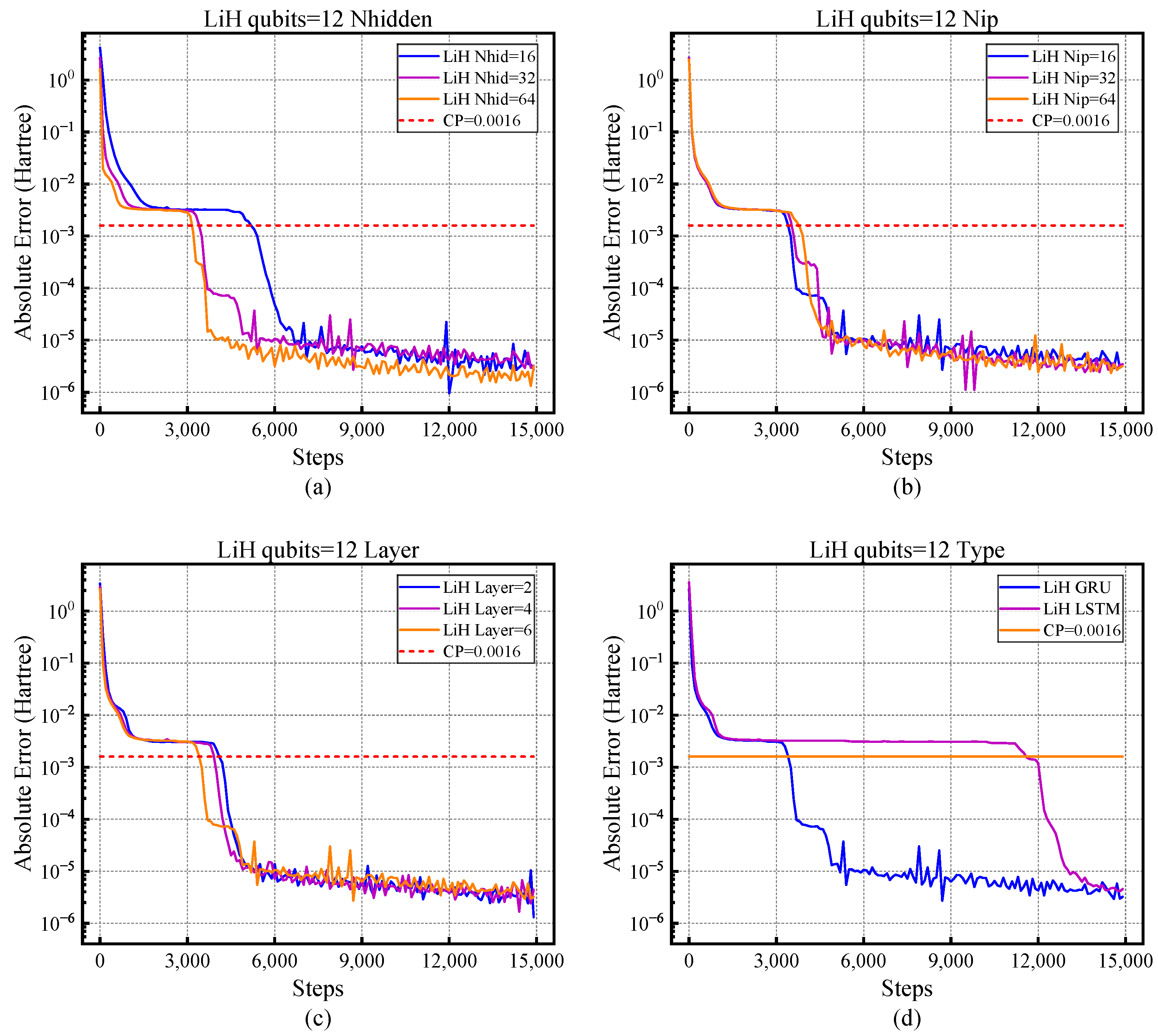
4.1. The Influence of Different Hyper-Parameters on NNQS

After a neural network model is built, it is typically fine-tuned through hyper-parameter tuning to enhance its expressive capability. In our study, we introduce the NNQS model, which possesses the following hyper-parameters: n_hidden, indicating the number of neurons in each hidden layer of the NNQS network; nip, representing the number of features in the input data; and in the context of NNQS, this denotes the representation of each qubit using a nip-dimensional vector; layer, signifying the number of layers in the NNQS network. The network-type parameter is employed to select between the gated recurrent unit (GRU) [39] and long short-term memory (LSTM) [40] is used for training. LSTM, a specialized form of recurrent neural network(RNN), is designed to address the long-term dependency issues encountered by a standard RNN in processing long sequences. Conversely, GRU, a variant of LSTM, combines the forget and input gates of LSTM into a single “update gate”, and it also merges the cell state with the hidden state, alongside other modifications. Due to its relatively simpler structure, GRU offers a higher computational efficiency. When testing the NNQS, we found that for molecular systems with more than 30 orbitals (qubits), the NNQS converged slowly and had difficulty converging to chemical precision (CP = 0.0016). Our goal was to choose a set of parameters that enabled better convergence for most systems. On an Nvidia A100 GPU with 40G of GPU memory, we meticulously tuned hyper-parameters such as n_hidden, nip, layer, and network-type. In addition, we used Pytorch 1.13.1 + cu116, Julia 1.8.0 to build our NNQS model.
Initially, we chose a small molecule system, LiH (qubit = 12), with less than 20 qubits for the hyper-parameter testing of our NNQS model. We selected LiH as the subject for our hyper-parameter testing due to its rapid computational efficiency, limited number of configurations, and suitability for streamlined parameter optimization and debugging processes. In Figure 4, the x-axis represents the iteration count of the NNQS model, while the y-axis shows the absolute error in energy at each step for LiH compared to FCI. When the absolute error diverged from the chemical precision (CP = 0.0016, denoted by the red dashed line in Figure 4), we considered the model to have converged.
Figure 4a demonstrates that the convergence performance for n_hidden = 64 was similar to that for n_hidden = 32, but the computational time per step was longer than n_hidden = 32. When n_hidden = 16, the model exhibited inferior convergence performance (indicated by the blue solid line in Figure 4a). In the second set of tests, it is shown that for nip = 16, 32, 64, the convergence curves are similar, but nip = 16 required a shorter computation time per step. Figure 4c reveals that at layer = 6, the model achieved chemical precision earlier (below the red dashed line), indicating a better convergence performance. Figure 4d illustrates that for the NNQS model, employing GRU resulted in a superior fit compared to LSTM. In summary, considering both the convergence performance and operational speed, we used n_hidden = 32, nip = 16, layer = 6, and GRU for subsequent testing
We compare our test results with the NAQS [17], RBM, and FCI in Table 1. The results show that our tested approach achieved a better convergence in certain systems and the data with a dark underline indicate the best values.

4.2. The Influence of DMRG Pre-Training on NNQS

In this section, we demonstrate the use of DMRG configuration coefficients as pre-training data for the NNQS. This approach enables supervised learning for the NNQS model, aiming to closely approximate the wave function predicted by DMRG before proceeding to inference. The checkpoints generated at different steps during the pre-training process have varying impacts on the model. A lower number of pre-training steps might result in suboptimal model fitting, leading to slower convergence and a higher initial inference energy during inference. Conversely, an excessive number of pre-training steps may lead to overfitting, where the model accurately fits the DMRG pre-training data’s wave function but may struggle to generate new samples or may exhibit stagnant energy levels during the subsequent inference. In such cases, we describe the NNQS as converging to a local minimum. We use the configuration coefficients generated using DMRG data to pre-train the NNQS. At first, we verify the convergence effect of this method with two smaller systems H 2 O (14 qubits) and H 10 STO-6G(20 qubits), as shown in Figure 5.
We selected the H 2 O and H 10 STO-6G systems to test the effectiveness of pre-training. Figure 5a,b represent the convergence of the H 10 STO-6G system, while (c,d) depict the convergence of H 2 O . The y-axis in Figure 5a,c shows the absolute error between the energy values inferred by the NNQS and those of the FCI, with the red dashed line representing the chemical precision. When the curve converged below this red dashed line, we considered the model to have inferred the energy of the molecular system with an accuracy acceptable by FCI standards. The y-axis in Figure 5b,d displays the actual energy values inferred by our NNQS model. We compare the energy values at the 1000-th (purple solid line), 2000-th (yellow solid line), and 3000-th (green solid line) pre-training steps checkpoints with those obtained from inference without pre-training (blue solid line). The experiment showed that for H 10 STO-6G, the energy in the first step of pre-training was lower than that of starting from scratch, as shown in Table 2. However, for the strongly correlated H 10 STO-6G system, the opposite was observed; the first step energy from scratch was erroneous, and the energy became accurate only after pre-training. For the 1000-th step checkpoints, the H 10 STO-6G system exhibited an abnormal convergence curve (purple solid line in Figure 5a,b), where the energy after pre-training was higher than that without pre-training (blue solid line), indicating overfitting of the model. Both H 10 STO-6G and H 2 O converged more quickly to chemical precision (below the red dashed line) after pre-training, demonstrating that using DMRG as a pre-training method for NNQS can accelerate its convergence.
As shown in Table 3 and Table 4, we compiled the number of iterations required for H 10 STO-6G and H 2 O to converge to chemical precision. For the unpretrained tests, we calculated the total runtime from scratch inference to convergence to chemical precision as the convergence time. For the pretrained tests, we recorded the time from the beginning of pretraining to the generation of the corresponding step’s checkpoint, and the time from loading the checkpoint to convergence to chemical precision as the convergence time. The results indicate that the convergence time and the number of iterations for the NNQS after pretraining were generally less than those for the unpretrained versions.
As depicted in Figure 6, DMRG data were employed for the pre-training of the NNQS. This pre-training notably enhanced the convergence trajectory for C 2 H 4 O , as evidenced by a marked decline. The convergence curve without pre-training is illustrated by the blue solid line in Figure 6. Evaluations were conducted utilizing DMRG checkpoints at the 20,000-th, 40,000-th, and 80,000-th steps. As delineated in Figure 6b , the unpretrained curve exhibits a discrepancy exceeding 0.02 relative to DMRG at the 29,000-th step (as indicated by the blue solid line). Furthermore, the energy extrapolated from the 20,000-th step checkpoint surpasses that derived from the 40,000-th and 80,000-th iteration checkpoints. The convergence curves of energy for the 40,000-th and 80,000-th iterations demonstrate similarity, suggesting a negligible variation in model parameters between these iterations in the pre-training phase. Figure 6a reveals that the initial energy inferred without pre-training (−134.756129) significantly exceeded the initial energies with pre-training (20,000-th checkpoint: −149.3210498, 40,000-th checkpoint: −149.337339, 80,000-th checkpoint: −149.344904).

4.3. The Influence of the Optimizer on NNQS

Numerous experiments have been conducted to investigate the effects of different optimizers on the calculation of wave functions using neural networks. Traditional first-order optimization algorithms, commonly used in these calculations, such as Adam [37], and AdamW [36], depend on the loss function’s first-order derivatives to minimize the loss. In contrast, second-order optimization algorithms, including Newton’s method and the LBFGS [41] optimizer, incorporate a Hessian matrix of the loss function. However, the computational challenges associated with computing and storing the Hessian matrix have impeded their widespread use.
At present, the Kronecker-factored approximate curvature (KFAC) optimizer has proven its efficiency in accelerating neural network convergence by leveraging approximations of the Hessian matrix, without imposing substantial computational overheads [42]. This method has been well tested and has shown great results in quantum chemistry computations [43,44]. However, when interfacing with certain complex network layers in PyTorch, the KFAC implementation requires specific layer formatting, which can pose challenges in its applicability. This has driven us to explore simpler second-order optimization algorithms that better fit with these network designs and can improve training speed.
We chose AdamW as the optimizer for NNQS for the following reasons: (1) it employs a more intuitive weight decay strategy compared to the standard Adam optimizer, making it easier to fine-tune the weight decay hyper-parameters. This aids in mitigating the risk of overfitting during model training and enhances generalization performance; (2) it also typically exhibits a more stable convergence performance during training, particularly in deep neural networks. This contributes to reducing the training instability and overall training time; (3) the Adam optimizer may introduce biases in parameter updates during the initial stages of training, leading to training instability. AdamW, through its improved weight decay method, mitigates such biases, thereby accelerating model convergence.
Weight decay is a regularization technique employed in deep learning models to mitigate the risk of overfitting. Its function entails the addition of an extra penalty term to the loss function, penalizing the model’s weight parameters, thereby encouraging them to tend towards smaller values. This aids in preventing the model from overfitting the training data during the training process, ultimately enhancing its generalization performance. In our study, we selected four quantum systems with qubits less than or equal to 30 and investigated the impact of different weight decay values on the performance of the AdamW optimizer within the NNQS-model. As shown in Figure 7, when the weight decay was set to 0.003, all four molecular systems exhibited favorable convergence curves.

4.4. Application: Ferrocene

For the application, we studied the transition barrier energy between two structures of ferrocene (Fe(C5H5)2), as shown in Figure 8. Ferrocene is an important organometallic compound, and it has stimulated an explosion of interest in compounds of d-block metals with hydrocarbons. The 1973 Chemistry Nobel Prize was bestowed upon Ernst Otto Fischer and Geoffrey Wilkinson “for their pioneering work, performed independently, on the chemistry of the organometallic, so called sandwich compounds”. The “sandwich” structure of ferrocene consists of two cyclopentadienyl (Cp) rings bound to a central iron atom. There are two kinds of structures with a small energy difference, called eclipsed ferrocene with D5h symmetry and staggered conformer with D5d symmetry, and the staggered structure has a lower energy than the eclipsed structure [45]. The ground state of ferrocene is dominated by a single configurations, including the coupling of Fe and C orbitals [46]. We used cc-pVTZ-DK basis set and used the automated valence active space (AVAS) [47] method to generate the desired active orbitals by projecting the canonical molecule into the Fe d and C pz atomic orbitals (30 spin-orbitals). Using our method, we obtained the energy barrier between the two structures as 9.16 × 10 3 Hartree, while the best estimates from the CASCI method predicted 9.30 × 10 3 Hartree. We can see that chemical accuracy (1 kcal/mol = 0.0016 Hatree) was achieved with our method. These results gave us confidence in our method’s ability to deal with complex system with transition metals, and even strongly correlated materials.
We compiled the NNQS in hybrid single-precision and double-precision on a new generation Sunway supercomputer, Julia 1.6.5 and Pytorch 1.13 was used, which had been integrated with the underlying runtime and computing libraries; for example, the MPI communication library (3.2b2) customized for the interconnection network topology of the new-generation Sunway supercomputer, deeply optimized BLAS and LAPACK libraries (3.8), etc. We also used an AMD EPYC 7742 CPU and NVIDIA A100 PCIe 80GB for the CPU and GPU computation environments, respectively.

5. Conclusions

This study represents a significant advancement in the field of quantum many-body physics, addressing the critical challenge of the complexity of equations in physics and chemistry. By integrating the density-matrix renormalization group (DMRG) method with transformer-based neural networks, we introduced a novel approach that efficiently tackles the computational difficulties in solving complex quantum systems, especially those with strong correlations. Future work will focus on further refining these methods, extending their applicability to even more complex systems, and exploring the integration of emerging machine learning and quantum computing techniques, to continue advancing our understanding of the quantum world.

Author Contributions

Methodology, B.K., Y.T. and D.X.; software, Y.W.; validation, B.K., Y.F. and H.S.; resources, Y.F. and H.S.; data curation, B.K.; conceptualization, H.S.; writing—original draft, B.K. and D.X.; writing—review & editing, B.K., Y.T. and H.S. All authors have read and agreed to the published version of the manuscript.

Funding

This research was funded by National Natural Science Foundation of China grant numbers T2222026 and 22003073.

Data Availability Statement

The data that support the findings of this study are available from the corresponding author upon request.

Acknowledgments

The authors would like to thank the National Natural Science Foundation of China (T2222026 and 22003073) for supporting this work.

Conflicts of Interest

The authors declare no conflict of interest.

References

  1. Shepard, R. The Multiconfiguration Self-Consistent Field Method. In Advances in Chemical Physics; John Wiley & Sons, Ltd.: Hoboken, NJ, USA, 1987; pp. 63–200. [Google Scholar] [CrossRef]
  2. Bartlett, R.J.; Musiał, M. Coupled-cluster theory in quantum chemistry. Rev. Mod. Phys. 2007, 79, 291–352. [Google Scholar] [CrossRef]
  3. Coester, F.; Kümmel, H. Short-range correlations in nuclear wave functions. Nucl. Phys. 1960, 17, 477–485. [Google Scholar] [CrossRef]
  4. White, S.R. Density matrix formulation for quantum renormalization groups. Phys. Rev. Lett. 1992, 69, 2863–2866. [Google Scholar] [CrossRef] [PubMed]
  5. White, S.R.; Martin, R.L. Ab initio quantum chemistry using the density matrix renormalization group. J. Chem. Phys. 1999, 110, 4127–4130. [Google Scholar] [CrossRef]
  6. Boguslawski, K.; Marti, K.H.; Reiher, M. Construction of CASCI-type wave functions for very large active spaces. J. Chem. Phys. 2011, 134, 224101. [Google Scholar] [CrossRef]
  7. Luo, Z.; Ma, Y.; Liu, C.; Ma, H. Efficient Reconstruction of CAS-CI-Type Wave Functions for a DMRG State Using Quantum Information Theory and a Genetic Algorithm. J. Chem. Theory Comput. 2017, 13, 4699–4710. [Google Scholar] [CrossRef] [PubMed]
  8. Carleo, G.; Troyer, M. Solving the quantum many-body problem with artificial neural networks. Science 2017, 355, 602–606. [Google Scholar] [CrossRef] [PubMed]
  9. Choo, K.; Neupert, T.; Carleo, G. Two-dimensional frustrated J1J2 model studied with neural network quantum states. Phys. Rev. B 2019, 100, 125124. [Google Scholar] [CrossRef]
  10. Sharir, O.; Levine, Y.; Wies, N.; Carleo, G.; Shashua, A. Deep Autoregressive Models for the Efficient Variational Simulation of Many-Body Quantum Systems. Phys. Rev. Lett. 2020, 124, 020503. [Google Scholar] [CrossRef] [PubMed]
  11. Schmitt, M.; Heyl, M. Quantum Many-Body Dynamics in Two Dimensions with Artificial Neural Networks. Phys. Rev. Lett. 2020, 125, 100503. [Google Scholar] [CrossRef]
  12. Yuan, D.; Wang, H.R.; Wang, Z.; Deng, D.L. Solving the Liouvillian Gap with Artificial Neural Networks. Phys. Rev. Lett. 2021, 126, 160401. [Google Scholar] [CrossRef] [PubMed]
  13. Zhao, X.; Li, M.; Xiao, Q.; Chen, J.; Wang, F.; Shen, L.; Zhao, M.; Wu, W.; An, H.; He, L.; et al. AI for Quantum Mechanics: High Performance Quantum Many-Body Simulations via Deep Learning. In Proceedings of the SC22: International Conference for High Performance Computing, Networking, Storage and Analysis, Dallas, TX, USA, 13–18 November 2022; pp. 1–15. [Google Scholar] [CrossRef]
  14. Pfau, D.; Spencer, J.S.; Matthews, A.G.D.G.; Foulkes, W.M.C. Ab initio solution of the many-electron Schrödinger equation with deep neural networks. Phys. Rev. Res. 2020, 2, 033429. [Google Scholar] [CrossRef]
  15. Hermann, J.; Schätzle, Z.; Noé, F. Deep-neural-network solution of the electronic Schrödinger equation. Nat. Chem. 2020, 12, 891–897. [Google Scholar] [CrossRef] [PubMed]
  16. Choo, K.; Mezzacapo, A.; Carleo, G. Fermionic neural-network states for ab-initio electronic structure. Nat. Commun. 2020, 11, 2368. [Google Scholar] [CrossRef] [PubMed]
  17. Barrett, T.D.; Malyshev, A.; Lvovsky, A. Autoregressive neural-network wavefunctions for ab initio quantum chemistry. Nat. Mach. Intell. 2022, 4, 351–358. [Google Scholar] [CrossRef]
  18. Wu, Y.; Xu, X.; Poletti, D.; Fan, Y.; Guo, C.; Shang, H. A Real Neural Network State for Quantum Chemistry. Mathematics 2023, 11, 1417. [Google Scholar] [CrossRef]
  19. Wu, Y.; Guo, C.; Fan, Y.; Zhou, P.; Shang, H. NNQS-Transformer: An Efficient and Scalable Neural Network Quantum States Approach for Ab Initio Quantum Chemistry. In Proceedings of the International Conference for High Performance Computing, Networking, Storage and Analysis, Denver, CO, USA, 12–17 November 2023; Association for Computing Machinery: New York, NY, USA, 2023. [Google Scholar] [CrossRef]
  20. Shang, H.; Guo, C.; Wu, Y.; Li, Z.; Yang, J. Solving Schrödinger Equation with a Language Model. arXiv 2023, arXiv:2307.09343. [Google Scholar]
  21. Nomura, Y.; Darmawan, A.S.; Yamaji, Y.; Imada, M. Restricted Boltzmann machine learning for solving strongly correlated quantum systems. Phys. Rev. B 2017, 96, 205152. [Google Scholar] [CrossRef]
  22. Huang, L.; Wang, L. Accelerated Monte Carlo simulations with restricted Boltzmann machines. Phys. Rev. B 2017, 95, 035105. [Google Scholar] [CrossRef]
  23. Deng, D.L.; Li, X.; Das Sarma, S. Quantum Entanglement in Neural Network States. Phys. Rev. X 2017, 7, 021021. [Google Scholar] [CrossRef]
  24. Cai, Z.; Liu, J. Approximating quantum many-body wave functions using artificial neural networks. Phys. Rev. B 2018, 97, 035116. [Google Scholar] [CrossRef]
  25. Choo, K.; Carleo, G.; Regnault, N.; Neupert, T. Symmetries and Many-Body Excitations with Neural-Network Quantum States. Phys. Rev. Lett. 2018, 121, 167204. [Google Scholar] [CrossRef]
  26. Vogiatzis, K.D.; Ma, D.; Olsen, J.; Gagliardi, L.; de Jong, W.A. Pushing configuration-interaction to the limit: Towards massively parallel MCSCF calculations. J. Chem. Phys. 2017, 147, 184111. [Google Scholar] [CrossRef]
  27. Ma, H.; Liu, J.; Shang, H.; Fan, Y.; Li, Z.; Yang, J. Multiscale quantum algorithms for quantum chemistry. Chem. Sci. 2023, 14, 3190–3205. [Google Scholar] [CrossRef]
  28. McClean, J.R.; Boixo, S.; Smelyanskiy, V.N.; Babbush, R.; Neven, H. Barren plateaus in quantum neural network training landscapes. Nat. Commun. 2018, 9, 4812. [Google Scholar] [CrossRef]
  29. Anschuetz, E.R.; Kiani, B.T. Beyond Barren Plateaus: Quantum Variational Algorithms Are Swamped with Traps. arXiv 2022, arXiv:2205.05786. [Google Scholar]
  30. Schollwöck, U. The density-matrix renormalization group in the age of matrix product states. Ann. Phys. 2011, 326, 96–192. [Google Scholar] [CrossRef]
  31. Mitrushchenkov, A.O.; Fano, G.; Linguerri, R.; Palmieri, P. On the importance of orbital localization in QC-DMRG calculations. Int. J. Quantum Chem. 2012, 112, 1606–1619. [Google Scholar] [CrossRef]
  32. Li, Z.; Chan, G.K.L. Spin-Projected Matrix Product States: Versatile Tool for Strongly Correlated Systems. J. Chem. Theory Comput. 2017, 13, 2681–2695. [Google Scholar] [CrossRef] [PubMed]
  33. Wouters, S.; Van Neck, D. The density matrix renormalization group for ab initio quantum chemistry. Eur. Phys. J. D 2014, 68, 272. [Google Scholar] [CrossRef]
  34. Chan, G.K.L.; Sharma, S. The Density Matrix Renormalization Group in Quantum Chemistry. Annu. Rev. Phys. Chem. 2011, 62, 465–481. [Google Scholar] [CrossRef] [PubMed]
  35. Xie, Z.; Song, Y.; Peng, F.; Li, J.; Cheng, Y.; Zhang, L.; Ma, Y.; Tian, Y.; Luo, Z.; Ma, H. Kylin 1.0: An ab-initio density matrix renormalization group quantum chemistry program. J. Comput. Chem. 2023, 44, 1316–1328. [Google Scholar] [CrossRef]
  36. Loshchilov, I.; Hutter, F. Decoupled Weight Decay Regularization. In Proceedings of the International Conference on Learning Representations, New Orleans, LA, USA, 6–9 May 2019. [Google Scholar]
  37. Kingma, D.P.; Ba, J. Adam: A Method for Stochastic Optimization. arXiv 2017, arXiv:1412.6980. [Google Scholar]
  38. Vaswani, A.; Shazeer, N.; Parmar, N.; Uszkoreit, J.; Jones, L.; Gomez, A.N.; Kaiser, L.; Polosukhin, I. Attention Is All You Need. arXiv 2017, arXiv:1706.03762. [Google Scholar]
  39. Cho, K.; van Merrienboer, B.; Gulcehre, C.; Bougares, F.; Schwenk, H.; Bengio, Y. Learning phrase representations using RNN encoder-decoder for statistical machine translation. In Proceedings of the Conference on Empirical Methods in Natural Language Processing (EMNLP 2014), Doha, Qatar, 25–29 October 2014. [Google Scholar]
  40. Graves, A. Long Short-Term Memory. In Supervised Sequence Labelling with Recurrent Neural Networks; Springer: Berlin/Heidelberg, Germany, 2012; pp. 37–45. [Google Scholar] [CrossRef]
  41. Liu, D.C.; Nocedal, J. On the limited memory BFGS method for large scale optimization. Math. Program. 1989, 45, 503–528. [Google Scholar] [CrossRef]
  42. Martens, J.; Grosse, R.B. Optimizing Neural Networks with Kronecker-factored Approximate Curvature. arXiv 2015, arXiv:1503.05671. [Google Scholar]
  43. von Glehn, I.; Spencer, J.S.; Pfau, D. A Self-Attention Ansatz for Ab-initio Quantum Chemistry. In Proceedings of the Eleventh International Conference on Learning Representations, Kigali, Rwanda, 1–5 May 2023. [Google Scholar]
  44. Schätzle, Z.; Szabó, P.B.; Mezera, M.; Hermann, J.; Noé, F. DeepQMC: An open-source software suite for variational optimization of deep-learning molecular wave functions. J. Chem. Phys. 2023, 159, 094108. [Google Scholar] [CrossRef]
  45. Harding, M.E.; Metzroth, T.; Gauss, J.; Auer, A.A. Parallel calculation of CCSD and CCSD (T) analytic first and second derivatives. J. Chem. Theory Comput. 2008, 4, 64–74. [Google Scholar] [CrossRef]
  46. Ishimura, K.; Hada, M.; Nakatsuji, H. Ionized and excited states of ferrocene: Symmetry adapted cluster—Configuration—Interaction study. J. Chem. Phys. 2002, 117, 6533–6537. [Google Scholar] [CrossRef]
  47. Sayfutyarova, E.R.; Sun, Q.; Chan, G.K.L.; Knizia, G. Automated construction of molecular active spaces from atomic valence orbitals. J. Chem. Theory Comput. 2017, 13, 4063–4078. [Google Scholar] [CrossRef]
Figure 1. Tensor network illustrating the evaluation of Ψ | H ^ | Ψ = E Ψ | Ψ (shown as (a)) and H ^ eff i | ψ i = λ | ψ i (shown as (b)). The green dots represent the MPSs, and the blue blocks represent the MPOs. The bonds linking certain tensors represent the tensor contraction operations between linked tensors over the corresponding dimension.
Mathematics 12 00433 g001
Figure 2. A brief illustration of the crossover (shown as (a)) and mutation (shown as (b)) operation. (a): the crossover step will combine the alpha spin configuration of a selected SD and the beta spin configuration of another selected SD to construct a new SD. (b): the mutation step will randomly choose an occupied spin orbital and excite to a randomly chosen unoccupied orbital.
Mathematics 12 00433 g002
Figure 3. The NNQS initially loads the state information from the DMRG pre-trained data. Then, it infers the psi values through model inference and computes the loss by comparing with the psi of DMRG. Parameter updates are conducted via the model’s optimizer. This process iterates, yielding step information at the time of checkpoint creation, loss value information at checkpoint generation, and the checkpoint files.
Mathematics 12 00433 g003
Figure 4. LiH hyper-parameter testing. The red dashed line represents chemical precision(CP), which is 0.0016. (a) the impact of different n _ h i d d e n on NNQS convergence. (b) the impact of different nips. (c) l a y e r indicates the number of layers in the NNQS model. (d) the impact of different network types on convergence performance.
Mathematics 12 00433 g004
Figure 5. (a,c) The absolute error between the NNQS network inference of H 2 O and H 10 STO-6G and FCI, with the red dashed line indicating the chemical precision (CP = 0.0016), (b,d) show the energy of NNQS network inference of H 2 O and H 10 STO-6G, with the red solid line indicating the corresponding FCI values.
Mathematics 12 00433 g005
Figure 6. Comparison of the convergence speed with and without pre-training for C 2 H 4 O . (a) The red dashed line represents chemical precision (CP = 0.0016) and the y-axis represents the absolute error between the inferred energy value and DMRG. (b) The red solid line represents the value of DMRG; the x-axis represents the number of training steps, and the y-axis represents the energy value.
Mathematics 12 00433 g006
Figure 7. Comparison of convergence rates for weight decay across the four systems (ad). The x-axis represents the number of training steps, and the y-axis represents the absolute energy comparison with FCI. The red dashed line indicates chemical precision (CP = 0.0016).
Mathematics 12 00433 g007
Figure 8. The eclipsed and staggered Ferrocene.
Mathematics 12 00433 g008
Table 1. Comparison of the energy (in Hartree) between this work, NAQS, RBM, and FCI.
Molecular SystemsThis WorkNAQSRBMFCI
LiH −7.7845−7.7845−7.7777−7.7845
H 2 O −75.0155−75.0155−74.9493−75.0155
N 2 −107.6599−107.6595−107.5440−107.6602
CH 4 −39.8062−39.8062−39.7571−39.8063
C 2 −74.6904−74.6899−74.5147−74.6908
LiF −105.1661−105.1662−105.1414−105.1662
PH 3 −338.6979−338.6984−338.6472−338.6984
Li 2 O −87.8916−87.8909−87.3660−87.8927
Table 2. Comparison of the first step energy between H 10 STO-6G and H 2 O with different pre-training steps.
Molecular Systems H 10 STO-6G H 2 O
no ckpt5.104793−69.437209
1000-th step ckpt−2.485850−73.123730
2000-th step ckpt−2.384864−73.343999
3000-th step ckpt−2.202542−73.386116
Table 3. Comparison of the elapse time between H 10 STO-6G and H 2 O with different pre-training steps.
Molecular Systems H 10 STO-6G H 2 O
no ckpt103.79351524.3876
1000-th step ckpt65.65471580.0200
2000-th step ckpt76.3441944.5145
3000-th step ckpt113.55181032.1916
Table 4. Comparison of the convergence step between H 10 STO-6G and H 2 O with different pre-training Steps.
Molecular Systems H 10 STO-6G H 2 O
no ckpt27327376
1000-th step ckpt8906925
2000-th step ckpt3472871
3000-th step ckpt5072358
Disclaimer/Publisher’s Note: The statements, opinions and data contained in all publications are solely those of the individual author(s) and contributor(s) and not of MDPI and/or the editor(s). MDPI and/or the editor(s) disclaim responsibility for any injury to people or property resulting from any ideas, methods, instructions or products referred to in the content.

