Article

Dynamically Meaningful Latent Representations of Dynamical Systems

by
Imran Nasim
1,2,* and
Michael E. Henderson
3
1
IBM Research Europe, Winchester SO21 2JN, UK
2
Department of Mathematics, University of Surrey, Guildford GU2 7XH, UK
3
IBM Research—Thomas J. Watson Research Center, New York, NY 10598, USA
*
Author to whom correspondence should be addressed.
Mathematics 2024, 12(3), 476; https://doi.org/10.3390/math12030476
Submission received: 18 December 2023 / Revised: 24 January 2024 / Accepted: 26 January 2024 / Published: 2 February 2024
(This article belongs to the Special Issue Applied Mathematics and Machine Learning)

Abstract

:
Dynamical systems are ubiquitous in the physical world and are often well-described by partial differential equations (PDEs). Despite their formally infinite-dimensional solution space, a number of systems have long time dynamics that live on a low-dimensional manifold. However, current methods to probe the long time dynamics require prerequisite knowledge about the underlying dynamics of the system. In this study, we present a data-driven hybrid modeling approach to help tackle this problem by combining numerically derived representations and latent representations obtained from an autoencoder. We validate our latent representations and show they are dynamically interpretable, capturing the dynamical characteristics of qualitatively distinct solution types. Furthermore, we probe the topological preservation of the latent representation with respect to the raw dynamical data using methods from persistent homology. Finally, we show that our framework is generalizable, having been successfully applied to both integrable and non-integrable systems that capture a rich and diverse array of solution types. Our method does not require any prior dynamical knowledge of the system and can be used to discover the intrinsic dynamical behavior in a purely data-driven way.

1. Introduction

Nonlinear partial differential equations (PDEs) are prevalent in physics and engineering, serving as powerful tools for describing complex phenomena that exhibit nonlinear behaviors and spatiotemporal chaos. These equations are often very difficult to probe due to the formally infinite dimensional solution space. Practically, this high dimensionality often obscures the underlying behavior of a dynamical system, leading to the model being both difficult to analyze and prohibitively expensive to use for predictions. However, learning a faithful lower-dimensional representation of the high-dimensional data is not a trivial task.
Due to the rapid progress in the field of deep learning, the construction of neural network-based models such as autoencoders has become a popular and powerful technique for non-linear manifold-based dimensionality reduction of PDEs [1,2]. Consequently, such progress has spurred significant endeavors to develop techniques that directly learn low-dimensional dynamical models from time series data [3,4,5,6,7]. Very recently, there has been some effort to use autoencoder-based architectures to estimate the intrinsic dimensionality of a dynamical system [8,9,10]. The motivation for this is largely based on the so-called Manifold Hypothesis, which posits that high-dimensional data often lie on or near low-dimensional manifolds [11]. The rigorous analysis of a number of physical systems seems to support this hypothesis [12,13]. Despite the formal infinite dimensionality of the PDE state space, dissipative systems are hypothesized to exhibit long-term behavior that converges to a finite-dimensional invariant manifold [14,15]. Clearly, understanding this invariant manifold is of critical importance as it plays a crucial role in determining the system’s overall dynamics over time. However, studying and classifying the long time dynamics of a dynamical system is a challenging task. In the case of comparatively simple and deterministic ordinary differential equations (ODEs), the dynamics may exhibit complicated behavior with strong random features commonly referred to as deterministic chaos [16,17,18]. This has prompted the development of many methods to investigate the cause of such behavior including, but not limited to, hyperbolic theory, bifurcation, and attractor theory [19,20,21]. PDEs are even more complex due to the presence of infinite-dimensional dynamics and require careful and sophisticated analysis methods [15,22,23]. This has led to the production of advanced analysis tools to probe the behavior of dynamical systems [24,25,26]. Although these tools offer great utility, they necessitate a prerequisite understanding of the underlying dynamics in order to effectively achieve the objective of ‘finding what you are looking for’. In this study, we aim to provide a hybrid approach using the autoencoder architecture and validating the inherent latent representations using mathematical representations derived from the numerical simulations of the system. We show that our approach captures the nature of the underlying dynamics for a variety of solution types. Additionally, we probe the question of what topological features are preserved in the latent representation with respect to the raw data using methods from persistent homology. A key part of our framework is that it is purely data-driven, enabling the technique to be used to discover the intrinsic dynamical behavior of systems without the need to have prerequisite knowledge about the underlying dynamics.
The structure of the paper is as follows. In Section 2, we introduce the mathematical models we consider in this study. In Section 3, we probe the long time dynamics of these models using numerical experiments. In Section 4, we introduce the autoencoder model architecture and present our results. Finally, in Section 6, we present our discussion.

2. Models

2.1. fKdV Equation

The forced Korteweg–de Vries (fKdV) is used, for example, to model weakly non-linear flow in a channel with a bump or disturbance in the channel depth [27]. There exists a number of possible solutions for a given type of disturbance. For simplicity, we will assume here no disturbance, which is equivalent to setting the forcing term to zero. Under this assumption, the fKdV can be written as [28]:
6 u t + u x x x + ( 9 u 6 ( F 1 ) ) u x = 0 ,
where F is the depth-based Froude number.
Let us assume an initial condition that takes the form u ( x , 0 ) = A cos k x + ϕ . Here, A, k, and ϕ are amplitude, wavenumber, and phase shift parameters, respectively.
Consider a transformation where v ( X , T ) = A u ( x , t ) and where X = k x and T = k t . We can now re-write the original fKdV in terms of our function v using the chain rule. This results in:
6 v T + k 2 v X X X + ( 9 A v 6 ( F 1 ) ) v X = 0 ,
where v ( X , 0 ) = cos ( X + ϕ ) . From Equation (2), we can see that the amplitude parameter A acts as a direct measure of the strength of the non-linear operator ( v v X ), whereas the wavenumber parameter squared ( k 2 ) is a measure with the strength of the third-order linear dispersive term ( v X X X ). We can define a relative non-linearity term κ where κ = A / k 2 from the reformulation given in Equation (2). We expect to be in a dispersive regime for small values of κ < 1 and to be in a nonlinear regime for κ 1 . The importance of this reformulation is that it allows us to consider a physically motivated set of initial conditions rather than some generic functional form. Note that Equation (2) is invariant to phase shifts. If v ( x , t ) is a trajectory, so is v ( x + ϕ , t ) .

2.2. Kuramoto–Sivashinksy Equation

The Kuramoto–Sivashinsky (KS hereafter) equation is a non-integrable, nonlinear PDE that can be used to model the evolution of surface waves and pattern formation for a number of physical systems [29]. The equation can be written as:
u t + u u x + u x x + ν u x x x x = 0 ,
where ν is a coefficient of viscosity. The KS equation captures the dynamics of spatio-temporal instabilities, such as those seen in flame fronts and fluid flows, and, due to non-integrability, gives rise to a rich array of long time dynamics for different values of ν . For example, in the case where ν = 16 71 , the KS equation exhibits bursting dynamics [30], whereas for ν = 16 337 , the KS equation exhibits beating traveling wave dynamics [31].

3. Long Time Dynamics

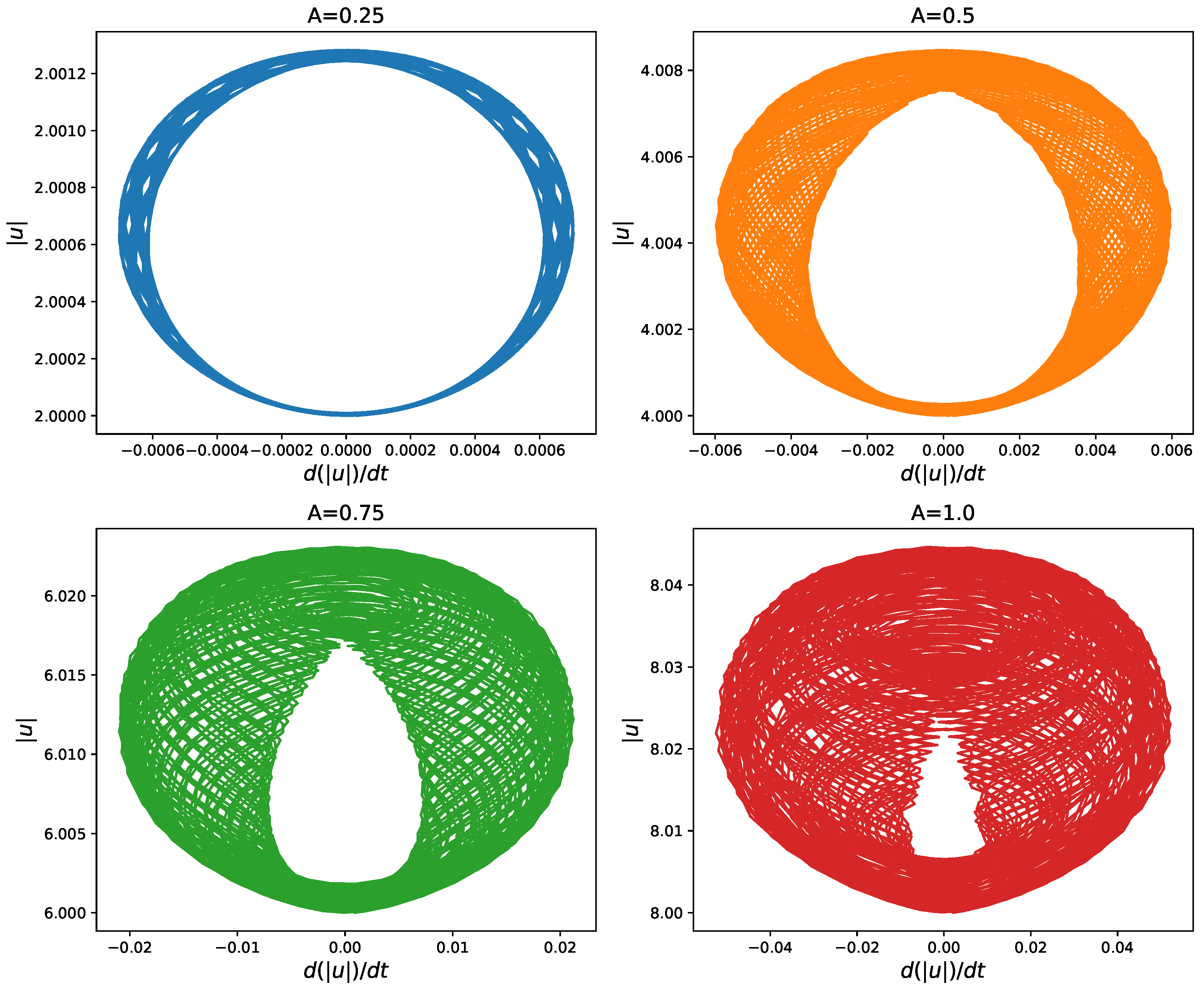
3.1. fKdV: Effects of Amplitude and Wavenumber

To investigate the nature of the long-term dynamics, we considered the fKdV under periodic boundary conditions with the domain of 2 π x 2 π ( L = 4 π ), and we considered an initial condition of the form u ( x , 0 ) = A cos k x + ϕ , where we fixed A = 0.5 , k = 1.0 and ϕ = 1.0 . We fixed the value of the Froude number F = 1.5 . All integrations were performed on a grid of 128 points using an explicit RK finite-difference scheme with a tolerance of 10 6 , which was compared to a pseudo-spectral method to ensure accuracy. To assess the effects of the amplitude and wavenumber, we chose two setups: (i) varying the amplitude and keeping the wavenumber and phase fixed (varying the phase under periodic conditions corresponds to a phase shift of the periodic domain and hence does not affect the dynamics; we also observed this within our simulations); and (ii) varying the wavenumber and keeping the amplitude and phase fixed. The integrations were performed for T = 400 units for amplitudes A ( 0 , 1 ] .
To visualize the trajectories, we consider the evolution of both the speed and distance as plotted in Figure 1. Interestingly, we observe that, for smallest amplitude case A = 0.25 , the evolution closely resembles a closed orbit, which is expected for a purely periodic motion (this was verified by running numerical integrations with smaller amplitudes). However, this characteristic changes significantly with increasing amplitude, where we observe quasi-periodic motion in speed–distance space. This behavior appears to correlate with the strength of the amplitude parameter, with larger amplitude initial conditions leading to non-periodicity. The quasi-periodic motion arises where two or more soliton frequencies are incommensurate [32]. We note that, for the transformed equation in Equation (2), the strength of this characteristic appears to correlate with the relative non-linearity term κ .
To further investigate this behavior, we proceeded to fix the amplitude and phase, then vary the value of the wavenumber k. The results for those numerical simulations are presented in Figure 2. Here, we observe that, when we increase the wavenumber by a factor of two, the initial quasi-periodic behavior quickly forms into a more pure periodic motion resembling circular motion in distance–speed space. This characteristic further supports the observation that the relative non-linearity essentially measures the strength of the quasi-periodicity, with weak relative non-linearity leading to pure periodic motion.

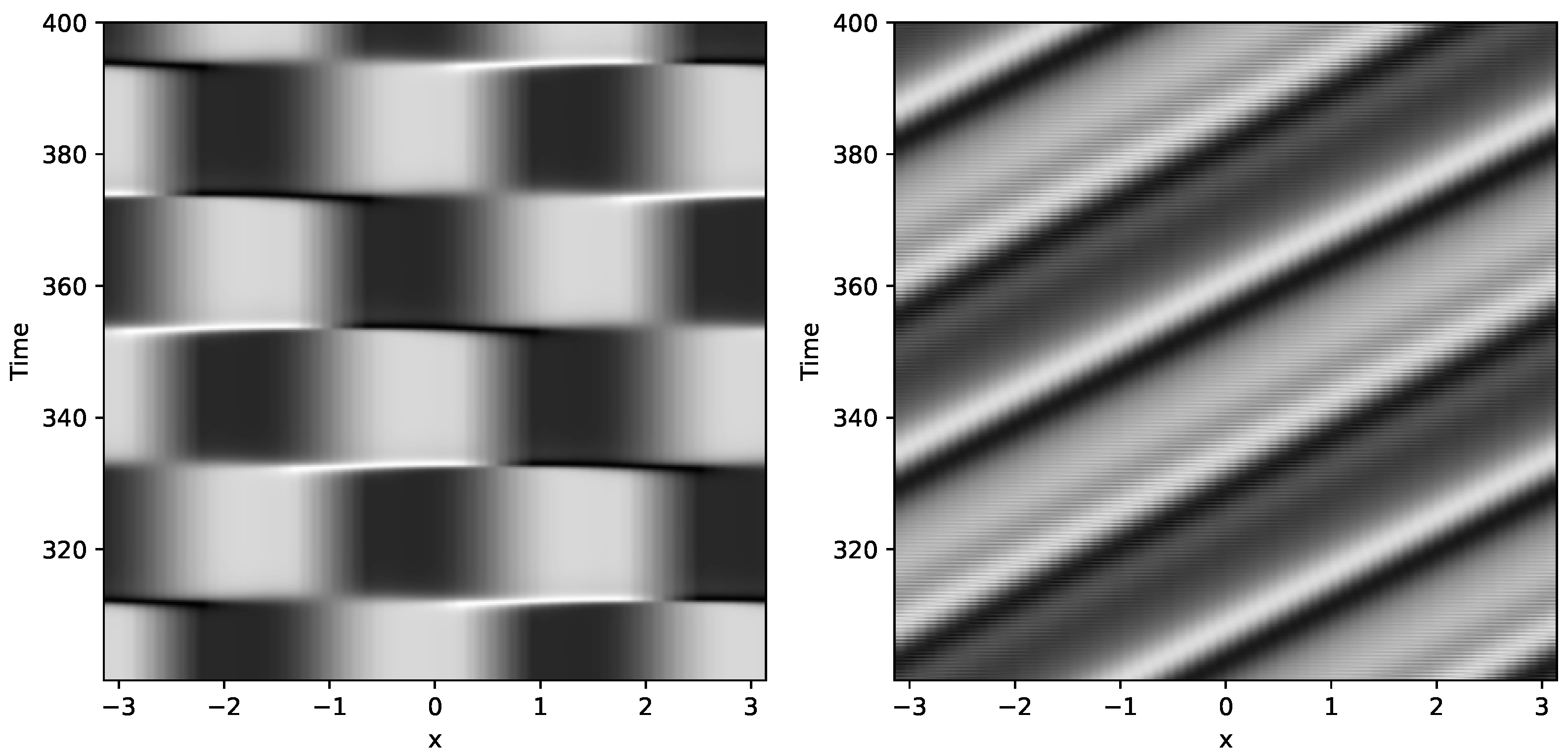
3.2. KS: Long Time Dynamics

We simulate the KS equation on a discretized grid with 64 grid points on a periodic domain π x π ( L = 2 π ). As with the fKdV setup, we considered an initial condition of the form u ( x , 0 ) = A cos k x + ϕ , where we fixed A = 0.5 , k = 1.0 , and ϕ = 1.0 . As we are interested in the long time dynamics, we evolved all models for T = 400 units to ensure all of the transients have died out. We consider two setups to reproduce the bursting dynamics and the beating traveling dynamics of the KS equation, setting ν = 16 71 and ν = 16 337 , respectively. We plot the long time evolution of the wave profiles in Figure 3.
From dynamical systems theory, we know that the bursting dynamics in the KS equation arise as the state appears to switch between two saddle points that are connected by four heteroclinic orbits [33]. This can be observed if we project the trajectory onto the two dominant Fourier modes, which is shown in the left panel of Figure 4. Here, we observe that this representation indeed captures the two saddle points and four heteroclinic connections. We observe that the trajectories tend to spend a majority of the time around the saddle points and appear to travel quickly on the heteroclinic connections pseudo-randomly, which supports the sudden bursting transitions seen in the wave profiles in Figure 3.
In the case of the beating traveling wave dynamics exhibited by the KS equation, we know that this dynamical behavior arises as the traveling period and beating period are out of phase [31]. This causes the orbit to follow quasi-periodic motion. To see if we are able to extract a low-dimensional representation that captures this characteristic, we project the trajectory into the two dominant Fourier modes, as shown in right panel of Figure 4. We clearly observe a quasi-periodic structure within this Fourier representation, which is supportive of the fact that the periodic orbit and beating period are incommensurate.

4. Interpretable Deep Learning-Based Reduced Order Model

Autoencoders have become a popular method for dimensionality reduction within the scientific community as a technique to obtain reduced order models. Autoencoders are incredibly versatile architectures. A single-layer autoencoder with a linear activation function is equivalent to Principal Component Analysis (PCA); however, multi-layered architectures with non-linear activations can perform complex non-linear dimensionality reduction. Fundamentally, autoencoders are composed of two deep neural networks, called the encoder and decoder, which are connected by a latent layer commonly referred to as the latent space. A schematic of a classical autoencoder is given in Figure 5.
This latent space is a bottleneck that sets the number of dimensions available to represent the input data. The encoder maps the inputs to the smaller latent space d z < d i ,
Φ E ( u ; θ E ) : R d i R d z ,
where θ E represents the parameters defining the encoder. The decoder maps the latent space back to: R d i
Φ D ( z ; θ D ) : R d z R d i .
The encoder reduces the dimension, and if the composition of these two mappings is the identity mapping, the decoder is the inverse of the encoder, and the encoding is one-to-one. For PCA, θ E is an orthonormal d z × ( d i + 1 ) matrix, Φ E ( u ) = θ E [ u 1 ] T , and Φ D ( u ) = [ u 1 ] θ E T . The extra dimension and the vector [ u 1 ] center the fit by adding a shift. Training the autoencoder on input/output pairs ( u , u ) minimizes the loss function in Equation (6) and forces Φ E and Φ D to be approximate inverses:
L ( u ; θ E ; θ D ) = u Φ D ( Φ E ( u ; θ E ) ; θ D ) 2 2 ,
where · 2 is the l 2 norm.
While autoencoders have obtained many impressive results, they are inherently data-driven, often leading to poor interpretability of the latent space. To probe the latent representation, we adopt a classical autoencoder architecture where the input data are the wave profile from our numerical simulation at each time interval t i . In the case of the fKdV models, this corresponds to input data u R 128 , where we consider a latent dimension d z = 3 that can be used to visualize the representation. For further details about the autoencoder model architecture and network parameters, please refer to Appendix A.

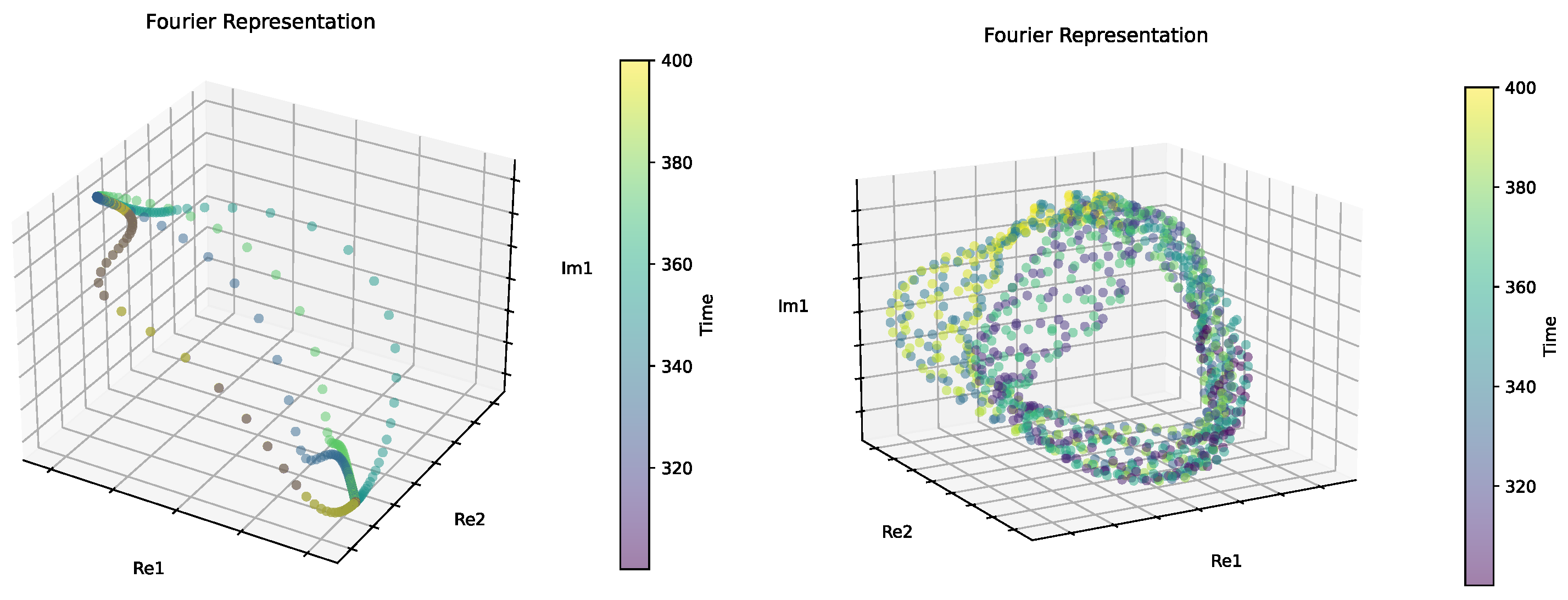
4.1. fKdV Latent Representation

A clear characteristic we inferred from the numerical simulations of the fKdV models presented in Section 3.1 was that the relative non-linearity term κ significantly influenced the type of long time dynamics, from purely periodic to strongly quasi-periodic. An important open question we aim to answer is whether the latent space of the autoencoder is able to capture and hence represent such qualitatively different dynamics. To this end, we construct the latent representation obtained from the suite of numerical simulations for the fKdV models with varying amplitudes. To focus on the representation of the long time dynamics, we train the autoencoder on the simulation data between T = 300 and T = 400 . We plot the original wave profile data with the corresponding latent representations in Figure 6. To our surprise, the representations obtained from the autoencoder appear to capture the qualitatively different dynamics, with the representations showing periodic motion for small amplitude models and quasi-periodic tori for larger amplitude cases (we confirmed this characteristic was present for the entire suite of numerical simulations we performed). This result is in direct agreement with the results obtained from analyzing the numerical simulations directly using the representation in distance–speed space. It is important to state that our autoencoder model is completely data-driven and has no prior information about the model being considered, yet it is able to extract representations that are dynamically meaningful.

4.2. KS Latent Representation

In Section 3.2, we described two dynamically distinct solution types to the KS equation, namely, the bursting dynamics and beating traveling dynamics. Using a projection onto the first few Fourier modes, we were able to obtain a low-dimensional representation that captured the dynamical characteristics of the full order numerical simulation in a dynamically interpretable way. A natural question we aim to answer in this section is whether we are able to extract an interpretable latent representation of these more complex dynamics using our autoencoder architecture. To tackle this question, we consider a similar approach to that which we used in the case of the fKdV. As we are focused on the long time dynamics, we train the autoencoder on the simulation data between T = 300 and T = 400 . The wave profiles from the numerical simulation with the corresponding latent space representations for the bursting and beating traveling dynamics are presented in Figure 7. Strikingly, we observe that the latent representation from the autoencoder trained on the bursting dynamics data almost perfectly resembles that of the Fourier representation we showed in Figure 4. This latent representation obtained from the autoencoder has captured the characteristics of the two saddle points in addition to the four heteroclinic connections, which is in direct agreement with the results obtained from the full numerical simulation. For the case of the beating traveling wave dynamics, the latent representation obtained from the autoencoder extracts a quasi-periodic representation in the latent space, which can be observed in the lower right panel of Figure 7. This quasi-periodic latent representation is in agreement with the dynamical theory and the numerically derived results in Section 3.2. It is important to note that, although the autoencoder is purely data-driven, the representation is clearly dynamically interpretable.

5. Topology Preservation

In the previous section, we have shown how we can use an autoencoder to obtain dynamically interpretable latent space embeddings, motivating the use of this architecture as a tool to probe the intrinsic dynamics in a purely data-driven way. However, while we have demonstrated the interpretability, we have not investigated the qualitative properties captured in the latent space with respect to the raw high-dimensional data. To address this question, we probe the nature of the topological features in both the raw data and latent representations using persistent homology. In the following subsection, we provide a very brief overview of the concepts used in this section to probe the topological features. For a deeper overview, we refer the reader to [34].

5.1. Persistent Homology

Topological data analysis gives away of classifying point clouds by connecting points across a range of scales and studying how the topology of the result changes. We give a broad overview of the technique below. A more detailed overview may be found in [35].
A classical way to represent the topology of discrete structures such as point clouds P is via simplicial complexes, which are a collection of smaller components called simplices. A 0-simplex is a single point, a 1-simplex an edge, and a 2-simplex a triangle with higher-order simplices having well-defined structures. Homology provides topologists with a formalized method for quantifying the presence of n-dimensional holes within a space [36]. The ith homology group H i ( P ) of P contains topological features of dimension i which, for the cases of d = 0 and d = 1 , are connected components and cycles/tunnels, respectively.
Persistent homology is a computational technique used in topological data analysis that takes in an input of increasing sequences of spaces ( P : P 0 P 1 P L ) referred to as a filtration. The idea behind persistent homology is that it extends the homology of simplicial complexes by considering the changes in homology groups over multiple scales of the distance metric, specifically connectivity-based features like connected components [34,37]. The common way this is done is via the construction of the Vietoris–Rips (VR) complex [38], which contains all the simplices of the point cloud at a given scale ϵ whose elements satisfy d i j < ϵ , where d i j is the distance metric between two points in the point cloud ( x i , x j P ). As the construction of the VR complex only requires the distances between points, it enables us to track changes in the homology groups for different ϵ values, up to a maximum value ϵ m , in which the connectivity remains the same. This enables us to obtain a measure of what homology groups are formed and destroyed at different ϵ values. A common way to visualize these features is via a persistence diagram. The i-dimensional persistence diagram of a VR complex contains coordinates of the form ( b , d ) , where b refers to the value at which a topological feature of dimension i is ‘birthed’ in the VR complex, and d refers to the value at which it has ‘died’. The intuition is that relevant topological characteristics, including connected components and voids associated with the Betti numbers for each simplex in the selected filtration, are monitored. It becomes possible to observe the duration of persistence of these topological features in the diagram as the parameter ϵ increases. Naturally, as the radius ϵ becomes sufficiently large, all pairs of points will fall within this radius, resulting in a single connected component and the absence of voids. To interpret the persistence diagram, each coordinate ( b , d ) denotes a topological feature being born at radius b and “dying” at radius d, where the death can be thought of as a homological feature getting filled in with a lower-dimensional simplex. From the diagram, one can measure the persistence of a feature that can be defined as d b . This value describes how “long”, with respect to radius, a topological feature exists before it is filled in.
A common way to measure the similarity between persistence diagrams is using the Wasserstein distance, which is a form of an optimal transport metric. The basic idea is that we can consider all possible transportation mechanisms for moving the points within one persistence diagram to the other one, a process called matching. A cost is associated with each transportation mechanism, where the distance is the infimum of these cost values [39]. Mathematically, it can be expressed as [40]:
W p ( d 1 , d 2 ) = inf γ ( x , y ) γ x y p 1 p ,
where γ ranges over all bijective mappings from persistence diagram d 1 to d 2 .

5.2. Persistence Diagrams

To compute and compare the persistence diagrams of both the raw higher-dimensional dynamical data and the latent representation obtained from the autoencoder, we restrict the analysis to homology groups up to the dimension of the latent space ( d = 3 ). We note that, while we expect higher-dimensional topological features to be present in the raw higher-dimensional data, these are not captured in the latent representation due to the reduced dimensionality. Hence, for comparative purposes, we do not consider this analysis. Figure 8 shows the persistence diagrams for the different dynamical models considered in this study, in which the left column represents the diagrams obtained from the raw data and the right column from the latent representation obtained via the autoencoder. In the case of the traveling wave fKdV data (upper panels), we observe the similarity in the grouping of distinct homology groups. There appears to be larger number of H 1 points from the latent data, but as these lie close to the Birth equals Death line, these are likely artifacts. More importantly, however, in both the raw and latent diagrams, there appears to be a single long persistent H 1 point showing a topological consistency. (The long persistent H 0 point on all diagrams is just an artifact of the algorithm and has no topological significance.) For the case of the KS bursting dynamics model, we observe a qualitatively identical persistence diagram between the raw and latent data. The distinct homology groupings match exceedingly well and clearly show the two persistent H 1 points in both diagrams. In the bottom panel of Figure 8, we observe the persistence diagrams of the KS beating dynamics. These diagrams appear slightly more complex compared to the other models, where the consistency between the raw and latent representations appears to be less well-defined. Upon closer inspection, we see the vast majority of points for both cases lie close to the Birth equals Death line and hence arise from noise. In the case of both the raw and latent representations, we see two long-persisting H 1 points, which shows topological agreement; however, we do notice a short time persistence H 2 point in the latent persistence diagram, which we do not observe in the profile of the raw data. Due to the short persistence, this feature is likely due to noise.
We then compute the Wasserstein distance between each pair of persistence diagrams for the different dynamical models. From this, we obtain W f K d V = 113.4 , W K S t = 260.6 , and W K S b = 5.3 , where the subscripts correspond to the models being considered, namely the fKdV, KS beating traveling wave, and KS bursting dynamics. These quantitative metrics support the qualitative features we observe in the persistence diagrams seen in Figure 8.
We acknowledge here that work has been done to include topology-preserving methodologies within the autoencoder architecture using the idea of persistence homology, perhaps most prominently by [41]. However, while this work proposes a topological loss term based on the topological differences between persistence diagrams of the input and latent data, the persistent homology of the vanilla autoencoder was not investigated. Additionally, it was found in this study that the MSE of the vanilla autoencoder generally outperformed the topological autoencoder. To our knowledge, the topological properties of the vanilla autoencoder architecture have not been investigated using persistent homology, and we believe we are the first to give empirical evidence in this area.

6. Discussion

In this study, we have developed a hybrid framework to probe the long time dynamics of dynamical systems using a combination of mathematical representations directly obtained from the numerical simulation data and the latent representation captured within the latent space of an autoencoder. The autoencoder architecture implemented in this study is purely data-driven and contains no prior information about the dynamics. In order to determine whether this framework can be generalized to arbitrary dynamical systems, we applied our methodology to both integrable and non-integrable systems that capture a rich and diverse array of solution types. Using the results from dynamical systems theory and mathematically motivated representations of the numerical simulation data, we validated that the latent representations from the autoencoder are in fact dynamically interpretable for qualitatively distinct dynamics. We show that the latent representations capture all of the qualitative dynamical characteristics present within the full order numerical simulation data though having a dimension significantly less than the full order data. We used this framework to help classify the long time dynamics of the fKdV equation using a physically motivated reformulation which, to our knowledge, is the first time this has been done. Additionally, we investigated the topological features in the latent representation of the autoencoder with respect to the raw data both qualitatively and quantitatively using persistent homology which, to our knowledge, is a novel contribution. It is important to note that this framework is generic in nature and provides clear and interpretable insights into the long time dynamics of PDE-based models without the need for vigorous mathematics. Additionally, a key part of our framework is that it does not require prior dynamical knowledge of the system being considered and hence can be used to discover the underlying dynamical behavior in a purely data-driven way. We hope to extend this framework to incorporate naturally derived geometrical information from PDE-based models, which we will present in a subsequent study.

Author Contributions

I.N. (Conceptualization: Lead; Data curation: Lead; Formal analysis: Lead; Funding acquisition: Lead; Investigation: Lead; Methodology: Lead; Project administration: Equal; Resources: Lead; Software: Lead; Supervision: Equal; Validation: Lead; Visualization: Lead; Writing—original draft: Lead; Writing—review & editing: Lead). M.E.H. (Methodology: Supporting; Supervision: Supporting; Validation: Supporting; Writing—review & editing: Supporting). All authors have read and agreed to the published version of the manuscript.

Funding

Imran Nasim acknowledges a UKRI Future Leaders Fellowship for support through the grant MR/T041862/1. The authors declare that no other funds, grants, or support were received during the preparation of this manuscript.

Data Availability Statement

The datasets generated during and/or analysed during the current study are available in the ‘Numerical Data for fkdv and KS equations’ repository, https://zenodo.org/records/10309413, accessed on 8 December 2023.

Conflicts of Interest

The authors declare no conflicts of interest.

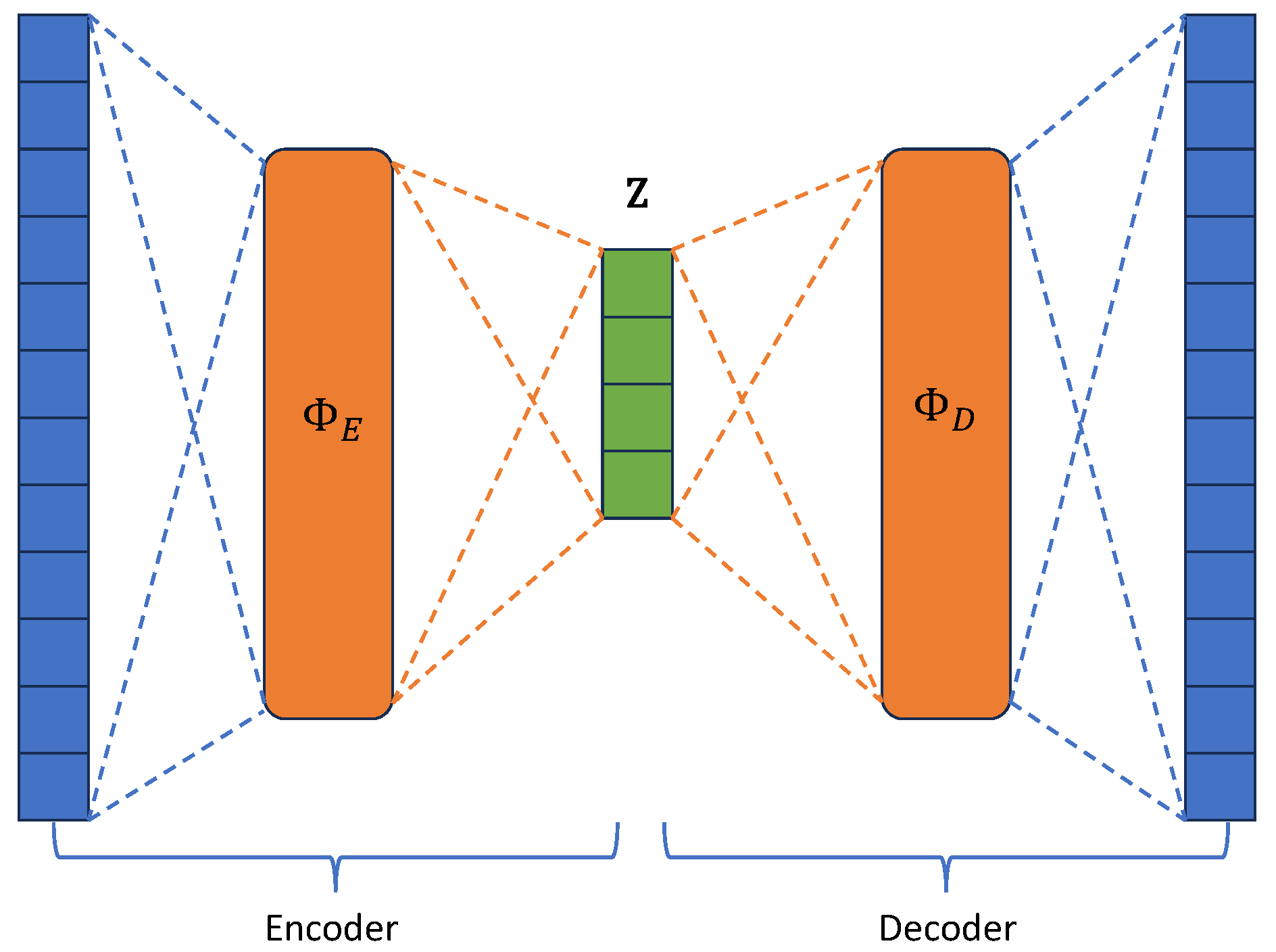
Appendix A. Autoencoder Model Architecture and Parameters

The parameters used in the autoencoder architecture are listed in Table A1. The autoencoders are trained using the Adam optimizer with a learning rate of 10 3 . All input data are MinMax scaled, which is why we use a Sigmoid activation function in the final layer of the decoder. The MSE of the training loss for all of the models presented in this study was on the order of magnitude of 10 4 .
Table A1. Parameters used in neural networks for the autoencoder where d i is the input dimension and d z is the latent dimension. The “Dimension” column describes the dimension of each layer, and the “Activation” column describes the activation functions between layers. The “Epochs” column describes the number of epochs used for training.
ComponentDimensionActivationsEpochs
Encoder d i :32:64:32: d z Linear:ReLU:Linear:ReLU:Linear1000
Decoder d z :32:64:32: d i Linear:ReLU:Linear:ReLU:Linear:Sigmoid1000

Appendix B. Bifurcation Classification of the fKdV

Here, we classify the bifurcation for the fKdV equation given in Equation (1) under the steady state assumption which, to our knowledge, has not been explicitly stated.
Let us consider the standard form of the fKdV given in Equation (1). In the case of traveling waves u ( x , t ) = u ( ϵ ) with ϵ = x c t and under the assumption of natural boundary conditions, we can turn this into a two-dimensional system that can be written as:
u = v v = 6 u ( c + F 1 ) 9 2 u 2 = h ( u ) .
To find the equilibrium points, we can solve v ( u ) = 0 , which leads to u 0 = 0 and u 1 = 4 3 ( c + F 1 ) . To classify these equilibrium points, we can solve the linearized equation J v = λ v . This results in det ( J λ ) , which can be expressed as:
det λ 1 h ( u ) λ .
Hence, the resulting characteristic equation is λ 2 h ( u ) = 0 .
This results in the eigenvalues λ 0 = ± 6 ( c + F 1 ) and λ 1 = ± ( 6 ( c + F 1 ) ) . The first eigenvalue λ 0 is purely imaginary if c + F < 1 and purely real if c + F > 1 , which is converse to the second eigenvalue λ 1 , which is purely imaginary if c + F > 1 and purely real if c + F < 1 . For the case of the two-equilibrium points u = 0 and u = 4 3 ( c + F 1 ) , the Jacobian has a double eigenvalue, which implies a Bogdanov–Takens bifurcation [42].

References

  1. Champion, K.; Lusch, B.; Kutz, J.N.; Brunton, S.L. Data-driven discovery of coordinates and governing equations. Proc. Natl. Acad. Sci. USA 2019, 116, 22445–22451. [Google Scholar] [CrossRef]
  2. Maulik, R.; Lusch, B.; Balaprakash, P. Reduced-order modeling of advection-dominated systems with recurrent neural networks and convolutional autoencoders. Phys. Fluids 2021, 33, 037106. [Google Scholar] [CrossRef]
  3. Brunton, S.L.; Proctor, J.L.; Kutz, J.N. Discovering governing equations from data by sparse identification of nonlinear dynamical systems. Proc. Natl. Acad. Sci. USA 2016, 113, 3932–3937. [Google Scholar] [CrossRef] [PubMed]
  4. Lusch, B.; Kutz, J.N.; Brunton, S.L. Deep learning for universal linear embeddings of nonlinear dynamics. Nat. Commun. 2018, 9, 4950. [Google Scholar] [CrossRef]
  5. Raissi, M.; Perdikaris, P.; Karniadakis, G. Physics-informed neural networks: A deep learning framework for solving forward and inverse problems involving nonlinear partial differential equations. J. Comput. Phys. 2019, 378, 686–707. [Google Scholar] [CrossRef]
  6. Lee, K.; Carlberg, K.T. Model reduction of dynamical systems on nonlinear manifolds using deep convolutional autoencoders. J. Comput. Phys. 2020, 404, 108973. [Google Scholar] [CrossRef]
  7. Linot, A.J.; Graham, M.D. Deep learning to discover and predict dynamics on an inertial manifold. Phys. Rev. E 2020, 101, 062209. [Google Scholar] [CrossRef] [PubMed]
  8. Schonsheck, S.; Chen, J.; Lai, R. Chart auto-encoders for manifold structured data. arXiv 2019, arXiv:1912.10094. [Google Scholar]
  9. Floryan, D.; Graham, M.D. Data-driven discovery of intrinsic dynamics. Nat. Mach. Intell. 2022, 4, 1113–1120. [Google Scholar] [CrossRef]
  10. Zeng, K.; Graham, M.D. Autoencoders for discovering manifold dimension and coordinates in data from complex dynamical systems. arXiv 2023, arXiv:2305.01090. [Google Scholar]
  11. Fefferman, C.; Mitter, S.; Narayanan, H. Testing the manifold hypothesis. J. Am. Math. Soc. 2016, 29, 983–1049. [Google Scholar] [CrossRef]
  12. Foias, C.; Sell, G.R.; Temam, R. Inertial manifolds for nonlinear evolutionary equations. J. Differ. Equ. 1988, 73, 309–353. [Google Scholar] [CrossRef]
  13. Temam, R.; Wang, X. Estimates On The Lowest Dimension Of Inertial Manifolds For The Kuramoto-Sivasbinsky Equation in The General Case. Differ. Integral Equ. 1994, 7, 1095–1108. [Google Scholar]
  14. Chepyzhov, V.V.; Višik, M.I. Attractors for Equations of Mathematical Physics; Number 49 in Colloquium Publications; American Mathematical Society: Providence, RI, USA, 2002. [Google Scholar]
  15. Zelik, S. Attractors. Then and now. arXiv 2022, arXiv:2208.12101. [Google Scholar]
  16. Tutueva, A.; Nepomuceno, E.G.; Moysis, L.; Volos, C.; Butusov, D. Adaptive Chaotic Maps in Cryptography Applications. In Cybersecurity: A New Approach Using Chaotic Systems; Abd El-Latif, A.A., Volos, C., Eds.; Springer International Publishing: Cham, Switzerland, 2022; pp. 193–205. [Google Scholar]
  17. Neamah, A.A.; Shukur, A.A. A Novel Conservative Chaotic System Involved in Hyperbolic Functions and Its Application to Design an Efficient Colour Image Encryption Scheme. Symmetry 2023, 15, 1511. [Google Scholar] [CrossRef]
  18. Li, R.; Lu, T.; Wang, H.; Zhou, J.; Ding, X.; Li, Y. The Ergodicity and Sensitivity of Nonautonomous Discrete Dynamical Systems. Mathematics 2023, 11, 1384. [Google Scholar] [CrossRef]
  19. Ruelle, D. Small random perturbations of dynamical systems and the definition of attractors. Commun. Math. Phys. 1981, 82, 137–151. [Google Scholar] [CrossRef]
  20. Katok, A.; Hasselblatt, B. Introduction to the Modern Theory of Dynamical Systems; Number 54; Cambridge University Press: Cambridge, MA, USA, 1995. [Google Scholar]
  21. Guckenheimer, J.; Holmes, P. Nonlinear Oscillations, Dynamical Systems, and Bifurcations of Vector Fields; Springer: Berlin/Heidelberg, Germany, 2013; Volume 42. [Google Scholar]
  22. Raugel, G. Global Attractors in Partial Diffenrential Equations; Département de Mathématique, Université de Paris-Sud: Orsay, France, 2001. [Google Scholar]
  23. Mielke, A.; Zelik, S.V. Infinite-Dimensional Hyperbolic Sets and Spatio-Temporal Chaos in Reaction Diffusion Systems in. J. Dyn. Differ. Equ. 2007, 19, 333–389. [Google Scholar] [CrossRef]
  24. Doedel, E.J.; Champneys, A.R.; Fairgrieve, T.; Kuznetsov, Y.; Oldeman, B.; Paffenroth, R.; Sandstede, B.; Wang, X.; Zhang, C. Auto-07p: Continuation and Bifurcation Software for Ordinary Differential Equations. 2007. Available online: http://indy.cs.concordia.ca/auto (accessed on 10 September 2023).
  25. Dhooge, A.; Govaerts, W.; Kuznetsov, Y.A.; Meijer, H.G.E.; Sautois, B. New features of the software MatCont for bifurcation analysis of dynamical systems. Math. Comput. Model. Dyn. Syst. 2008, 14, 147–175. [Google Scholar] [CrossRef]
  26. Dankowicz, H.; Schilder, F. Recipes for Continuation; SIAM: Philadelphia, PA, USA, 2013. [Google Scholar]
  27. Binder, B.; Vanden-Broeck, J.M. Free surface flows past surfboards and sluice gates. Eur. J. Appl. Math. 2005, 16, 601–619. [Google Scholar] [CrossRef]
  28. Binder, B.J. Steady Two-Dimensional Free-Surface Flow Past Disturbances in an Open Channel: Solutions of the Korteweg–De Vries Equation and Analysis of the Weakly Nonlinear Phase Space. Fluids 2019, 4, 24. [Google Scholar] [CrossRef]
  29. Kuramoto, Y. Diffusion-Induced Chaos in Reaction Systems. Prog. Theor. Phys. Suppl. 1978, 64, 346–367. [Google Scholar] [CrossRef]
  30. Kirby, M.; Armbruster, D. Reconstructing phase space from PDE simulations. Z. Angew. Math. Phys. 1992, 43, 999–1022. [Google Scholar] [CrossRef]
  31. Rowley, C.W.; Marsden, J.E. Reconstruction equations and the Karhunen–Loève expansion for systems with symmetry. Phys. D Nonlinear Phenom. 2000, 142, 1–19. [Google Scholar] [CrossRef]
  32. Lax, P.D. Almost periodic solutions of the KdV equation. SIAM Rev. 1976, 18, 351–375. [Google Scholar] [CrossRef]
  33. Kevrekidis, I.G.; Nicolaenko, B.; Scovel, J.C. Back in the saddle again: A computer assisted study of the Kuramoto–Sivashinsky equation. SIAM J. Appl. Math. 1990, 50, 760–790. [Google Scholar] [CrossRef]
  34. Otter, N.; Porter, M.A.; Tillmann, U.; Grindrod, P.; Harrington, H.A. A roadmap for the computation of persistent homology. EPJ Data Sci. 2017, 6, 1–38. [Google Scholar] [CrossRef]
  35. Chazal, F.; Michel, B. An Introduction to Topological Data Analysis: Fundamental and Practical Aspects for Data Scientists. Front. Artif. Intell. 2021, 4. [Google Scholar] [CrossRef]
  36. Rubio, J.; Sergeraert, F. Constructive algebraic topology. Bull. Des Sci. Math. 2002, 126, 389–412. [Google Scholar] [CrossRef]
  37. Edelsbrunner, H.; Letscher, D.; Zomorodian, A. Topological persistence and simplification. Discret. Comput. Geom. 2002, 28, 511–533. [Google Scholar] [CrossRef]
  38. Vietoris, L. Über den höheren Zusammenhang kompakter Räume und eine Klasse von zusammenhangstreuen Abbildungen. Math. Ann. 1927, 97, 454–472. [Google Scholar] [CrossRef]
  39. Skraba, P.; Turner, K. Wasserstein stability for persistence diagrams. arXiv 2020, arXiv:2006.16824. [Google Scholar]
  40. Mileyko, Y.; Mukherjee, S.; Harer, J. Probability measures on the space of persistence diagrams. Inverse Probl. 2011, 27, 124007. [Google Scholar] [CrossRef]
  41. Moor, M.; Horn, M.; Rieck, B.; Borgwardt, K. Topological autoencoders. Proc. Mach. Learn. Res. 2020, 119, 7045–7054. [Google Scholar]
  42. Kuznetsov, Y.A.; Kuznetsov, I.A.; Kuznetsov, Y. Elements of Applied Bifurcation Theory; Springer: New York, NY, USA, 1998; Volume 112. [Google Scholar]
Figure 1. Evolutions of trajectories in distance–speed space for initial conditions evolved under the fKdV equation for different initial amplitude values. A = 0.25 (upper left panel), A = 0.50 (upper right panel), A = 0.75 (lower left panel), A = 1.00 (lower right panel).
Mathematics 12 00476 g001
Figure 2. Evolutions of trajectories in distance–speed space for initial conditions evolved under the fKdV equation for different initial wavenumber values. k = 1.0 (left panel), k = 2.0 (right panel).
Mathematics 12 00476 g002
Figure 3. Long time wave profiles for the KS equation. Bursting dynamics (left panel) where ν = 16 71 , and beating traveling wave dynamics (right panel) where ν = 16 337 .
Mathematics 12 00476 g003
Figure 4. Fourier representation of the long time dynamics on the two leading spatial modes. Bursting dynamics (left panel) where ν = 16 71 , and beating traveling wave dynamics (right panel) where ν = 16 337 . Re1 and Re2 represent the real component of the first and second most dominant Fourier modes, respectively, while Im1 represents the imaginary component of the first dominant mode.
Mathematics 12 00476 g004
Figure 5. Schematic of the classical autoencoder architecture highlighting the encoder, decoder, and latent space (green) components.
Mathematics 12 00476 g005
Figure 6. Original wave profiles (left column) obtained from the numerical simulations of the fKdV and their corresponding latent space representations (right column) obtained using the autoencoder. Upper to lower plot: A = 0.11 , A = 0.26 , A = 0.47 .
Mathematics 12 00476 g006
Figure 7. Original wave profiles from the numerical simulation (left panels) and their corresponding latent representations obtained from the autoencoder. Bursting dynamics (upper panels) where ν = 16 71 and beating traveling wave dynamics (lower panels) where ν = 16 337 .
Mathematics 12 00476 g007
Figure 8. Persistence diagrams for the point cloud data from different dynamical models: (i) fkdv (upper panels); (ii) KS bursting dynamics (middle panels); (iii) KS beating traveling waves (lower panels). Results for the raw high-dimensional dynamical data (left column) and the latent representation obtained from the autoencoder (right column).
Mathematics 12 00476 g008
Disclaimer/Publisher’s Note: The statements, opinions and data contained in all publications are solely those of the individual author(s) and contributor(s) and not of MDPI and/or the editor(s). MDPI and/or the editor(s) disclaim responsibility for any injury to people or property resulting from any ideas, methods, instructions or products referred to in the content.

