Abstract
In this paper, two randomized block Kaczmarz methods to compute inner inverses of any rectangular matrix A are presented. These are iterative methods without matrix multiplications and their convergence is proved. The numerical results show that the proposed methods are more efficient than iterative methods involving matrix multiplications for the high-dimensional matrix.
MSC:
65F10; 65F45; 65H10
1. Introduction
Consider the linear matrix equation
where and . The solution X of (1) is called the inner inverse of A. For arbitrary , all the inner inverses of A can be expressed as
where is the Moore–Penrose generalized inverse of A.
Inner inverses play a role in solving systems of linear equations, finding solutions to least squares problems, and characterizing the properties of linear transformations [1]. They are also useful in various areas of engineering, such as robotics, big data analysis, network learning, sensory fusion, and so on [2,3,4,5,6].
To calculate the inner inverse of a matrix, various methods can be used, such as the Moore–Penrose pseudoinverse, singular value decomposition (SVD), or the method of partitioned matrices [1]. To our knowledge, few people discuss numerical methods for solving all the inner inverses of a matrix. In [7], the authors designed an iterative method based on gradient (GBMC) to solve the matrix Equation (1), which has the following iterative formula:
Here, is called the convergence factor. If the initial matrix , then the sequence converges to . Recently, various nonlinear and linear recurrent neural network (RNN) models have been developed for computing the pseudoinverse of any rectangular matrices (for more details, see [8,9,10,11]). The gradient-based neural network (GNN), whose derivation is based on the gradient of an nonnegative energy function, is an alternative for calculating the Moore–Penrose generalized inverses [12,13,14,15]. These methods for solving the inner inverses and for other generalized inverses of a matrix frequently use the matrix–matrix product operation, and consume a lot of computing time. In this paper, we aimed to explore two block Kaczmarz methods to solve (1) by the product of the matrix and vector.
In this paper, we denote , , , , and as the conjugate transpose, the Moore–Penrose pseudoinverse, the inner inverse, the 2-norm, the Frobenius norm of A and the inner product of two matrices A and B, respectively. In addition, for a given matrix , , , , and , are used to denote its ith row, jth column, the column space of A, the maximum singular value and the smallest nonzero singular value of A, respectively. Recall that and . For an integer , let . Let denote the expected value conditional on the first k iterations; that is,
where is the column chosen at the sth iteration.
The rest of this paper is organized as follows. In Section 2, we derive the projected randomized block Kaczmarz method (MII-PRBK) for finding the inner inverses of a matrix and give its theoretical analysis. In Section 3, we discuss the randomized average block Kaczmarz method (MII-RABK) and its convergence results. In Section 4, some numerical examples are provided to illustrate the effectiveness of the proposed methods. Finally, some brief concluding remarks are described in Section 5.
2. Projected Randomized Block Kaczmarz Method for Inner Inverses of a Matrix
The classical Kaczmarz method is a row iterative scheme for solving the linear consistent system that requires only cost per iteration and storage and has a linear rate of convergence [16]. At each step, the method projects the current iteration onto the solution space of a single constraint. In this section, we are concerned with the randomized Kaczmarz method to solve the matrix Equation (1). At the kth iteration, we find the next iterate that is closest to the current iteration in the Frobenius norm under the ith condition . Hence, is the optimal solution of the following constrained optimization problem:
Using the Lagrange multiplier method, turn (2) into the unconstrained optimization problem
Differentiating Lagrangian function with respect to X and setting to zero gives . Substituting into (3) and differentiating with respect to Y, we can obtain . So, the projected randomized block Kaczmarz for solving iterates as
where is selected with probability . We describe this method as Algorithm 1, which is called the MII-PRBK algorithm.
| Algorithm 1 Projected randomized block Kaczmarz method for matrix inner inverses (MII-PRBK) |
Input: ,
|
The following lemmas will be used extensively in this paper. Their proofs are straightforward.
Lemma 1.
Let be given. For any vector , it holds that
Lemma 2
([17]). Let be given. For any matrix , if , it holds that
Using Lemma 2 twice, and the fact , we can obtain Lemma 3.
Lemma 3.
Let be given. For any matrix , if and , it holds that
Remark 1.
Lemma 3 can be seen as a special case of Lemma 1 in [18]. That is, let For any matrix , it holds Notice that is well defined because and .
Theorem 1.
The sequence generated by the MII-PRBK method starting from any initial matrix converges linearly to in the mean square form. Moreover, the solution error in expectation for the iteration sequence obeys
where .
3. Randomized Average Block Kaczmarz Method for Inner Inverses of a Matrix
In practice, the main drawback of (4) is that each iteration is expensive and difficult to parallelize, since the Moore–Penrose inverse is needed to compute. In addition, is unknown or too large to store in some practical problem. It is necessary to develop the pseudoinverse-free methods to compute the inner inverses of large-scale matrices. In this section, we exploit the average block Kaczmarz method [16,19] for solving linear equations to matrix equations.
At each iteration, the PRBK method (4) does an orthogonal projection of the current estimate matrix onto the corresponding hyperplane . Next, instead of projecting on the hyperplane , we consider the approximate solution by projecting the current estimate onto the hyperplane . That is,
Then, we take a convex combination of all directions (the weight is ) with some stepsize , and obtain the following average block Kaczmarz method:
Setting , we obtain the following randomized block Kaczmarz iteration
where is selected with probability . The cost of each iteration of this method is if the square of the row norm of A has been calculated in advance. We describe this method as Algorithm 2, which is called the MII-RABK algorithm.
| Algorithm 2 Randomized average block Kaczmarz method for matrix inner inverses (MII-RABK) |
Input: , and
|
In the following theorem, with the idea of the RK method [20], we show that the iteration (11) converges linearly to the matrix for any initial matrix .
Theorem 2.
Assume . The sequence generated by the MII-RABK method starting from any initial matrix converges linearly to in mean square form. Moreover, the solution error in expectation for the iteration sequence obeys
where .
Proof.
It follows from
and
that
By taking the conditional expectation, we have
Noting that and , we have by induction. Then, by Lemma 3 and , we can obtain
Remark 2.
If or , then , which is the unique minimum norm least squares solution of (2). Theorems 1 and 2 imply that the sequence generated by the MII-PRBK or MII-RABK method with or converges linearly to .
Remark 3.
Noting that
this means that the convergence factor of the MII-PRBK method is smaller than that of MII-RABK method. However, in practice, it is very expensive to calculate the pseudoinverse of large-scale matrices.
Remark 4.
Replacing in (11) with , we obtain the following relaxed projected randomized block Kaczmarz method (MII-PRBKr)
where is the step size, and i is selected with probability . By the similar approach as used in the proof of Theorem 2, we can prove that the iteration satisfies the following estimate
where . It is obvious that when , the MII-PRBKr iteration (14) is actually the MII-PRBK iteration (4).
4. Numerical Experiments
In this section, we will present some experiment results of the proposed algorithms for solving the inner inverse, and compare them with GBMC [7] for rectangular matrices. All experiments are carried out by using MATLAB (version R2020a) in a personal computer with Intel(R) Core(TM) i7-4712MQ CPU @2.30 GHz, RAM 8 GB and Windows 10.
All computations are started with the random matrices , and terminated once the relative error (RE) of the solution, defined by
at the current iteration , satisfies or exceeds the maximum iteration . We report the average number of iterations (denoted as “IT”) and the average computing time in seconds (denoted as“CPU”) for 10 trials repeated runs of the MII-PRBK and MII-RABK methods. For clarity, we restate three methods as follows.
- GBMC ([7])
- MII-PRBK (Algorithm 1)
- MII-RABK (Algorithm 2)
We underscore once again the difference between the two algorithms; that is, Algorithm 1 needs the Moore–Penrose generalized inverse , whereas Algorithm 2 replaces with (which is easier to implement) and adds a stepsize parameter .
Example 1.
For given , the entries of A are generated from a standard normal distribution by a Matlab built-in function, i.e., or .
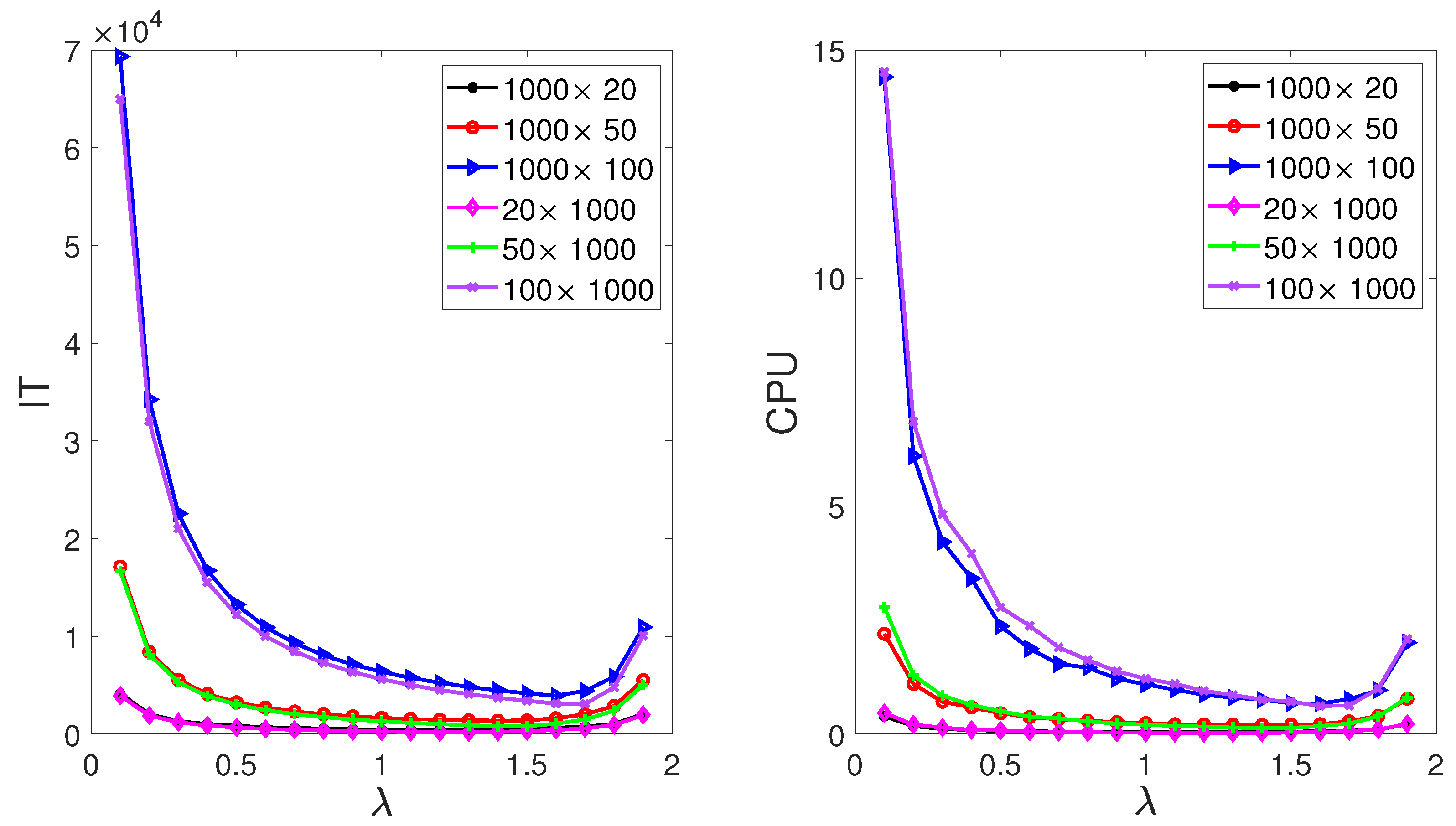
Firstly, we test the impact of in the MII-RABK method on the experimental results. To do this, we vary from to by step , where satisfies in Theorem 2. Figure 1 plots the IT and CPU versus different with different matrices in Table 1. From Figure 1, it can be seen that the number of iteration steps and the running time first decrease and then increase with the increase in , and almost achieve the minimum value when for all matrices. Therefore, we set in this example.
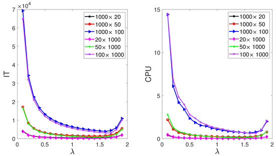
Figure 1.
IT (left) and CPU (right) of different of the RABK method for from Example 1.

Table 1.
The numerical results of IT and CPU for from Example 1.
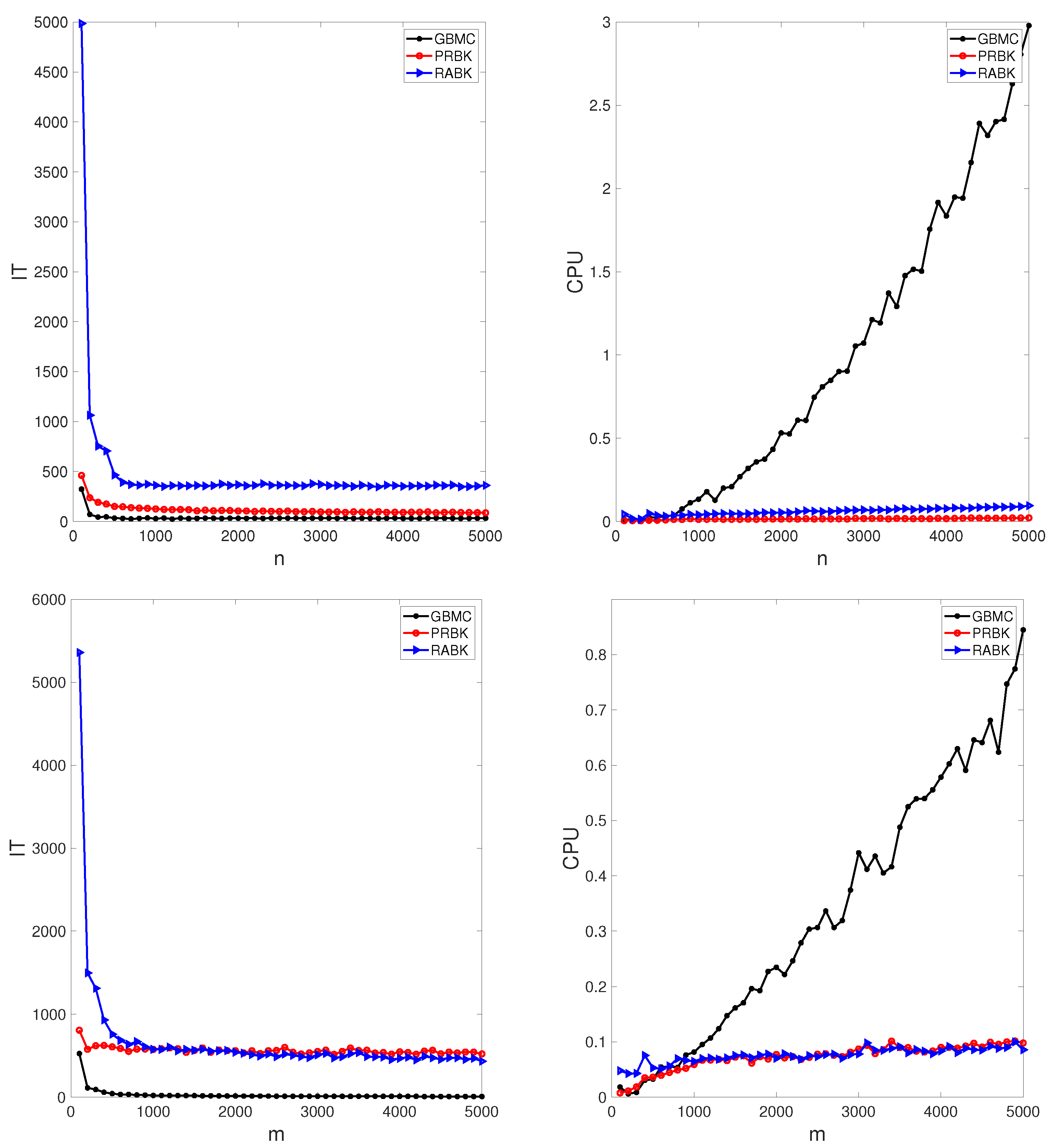
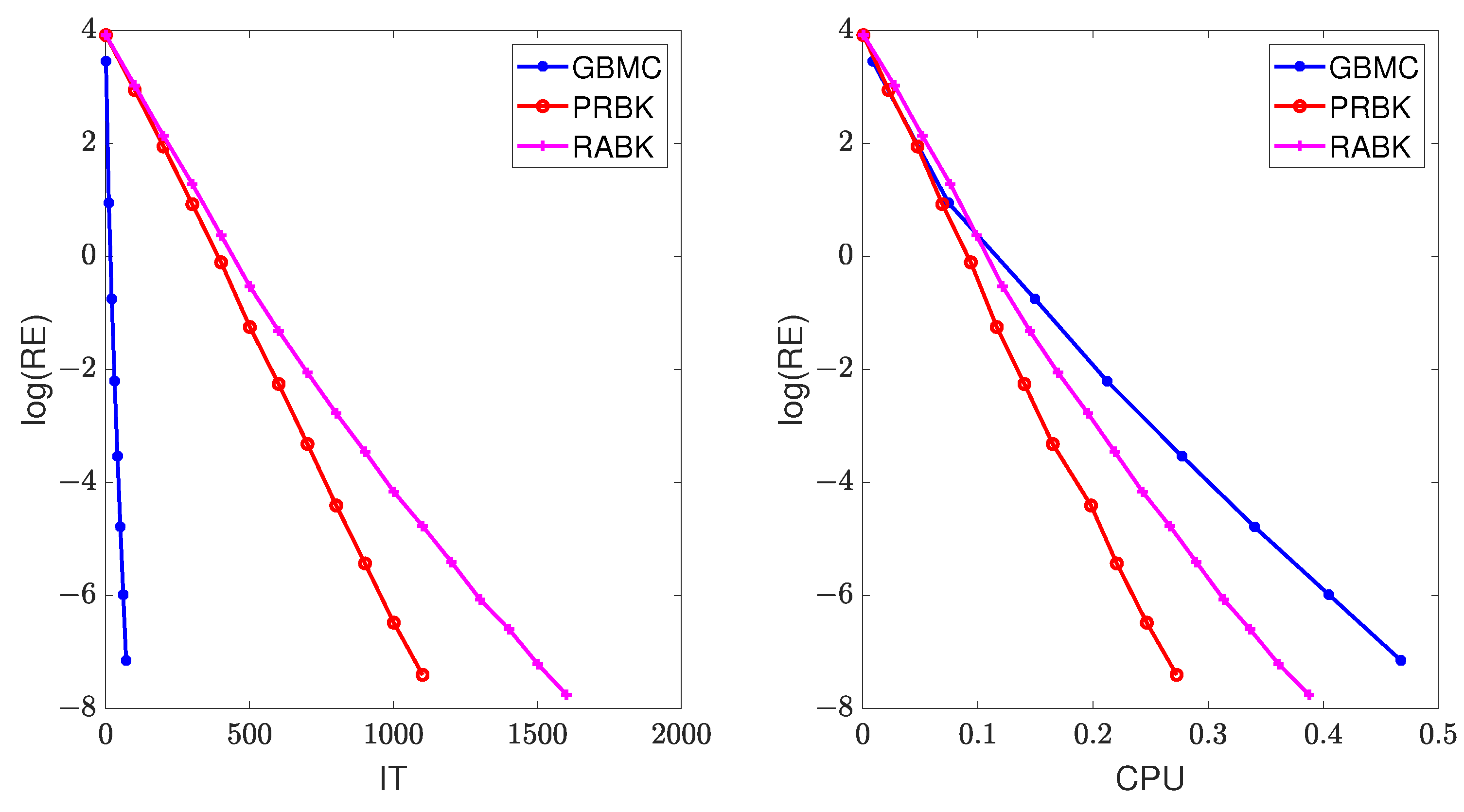
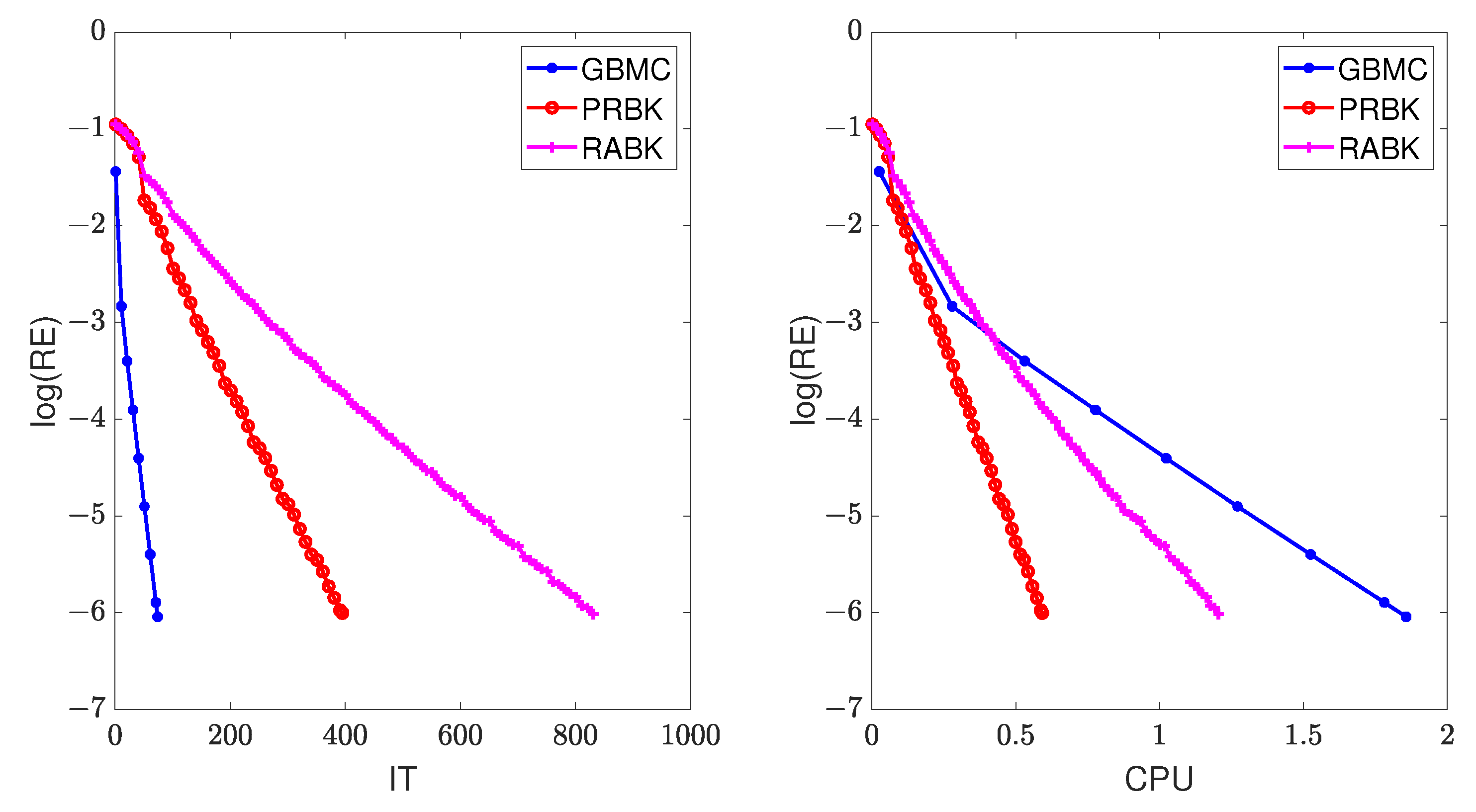
The results of numerical experiments are listed in Table 1 and Table 2. From these tables, it can be seen that the MII-GMBC method has the least number of iteration steps, whereas the MII-PRBK method has the least running time. Figure 2 plots the iteration steps and running time of different methods with the matrices (top) and (bottom). It is pointed out that the initial points on the left plots (i.e., and ) indicate that the MII-RABK method requires a very large number of iteration steps, which is related to Kaczmarz’s anomaly [21]. That is, the MII-RABK method enjoys a faster rate of convergence in the case where m is considerably smaller or larger than n. However, the closer m and n are, the slower the convergence is. As the number of rows or columns increases, the iteration steps and runtime of the MII-PRBK and MII-RABK methods are increasing relatively slowly, while the runtime of the GMBC method grows dramatically (see the right plots in Figure 2). Therefore, our proposed methods are more suitable for large matrices. The curves of relative error versus the number of iterations “IT” and running time “CPU”, given by the GMBC, MII-PRBK, MII-RABK methods for , are shown in Figure 3. From Figure 3, it can be seen that the relative error of GBMC method decays the fastest when the number of iterations increases and the relative error of MII-PRBK decays the fastest when the running time grows. This is because at each iteration, the GMBC method requires matrix multiplication which involves flopping operations, whereas the MII-PRBK and MII-RABK methods only cost flops.
Table 2.
The numerical results of IT and CPU for from Example 1.
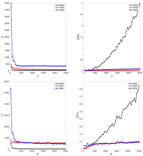
Figure 2.
IT (left) and CPU (right) of different methods with the matrices (top) and (bottom) from Example 1.

Figure 3.
The relative error of the different methods for .
Example 2.
For given , the sparse matrix A is generated by a Matlab built-in function , with approximately normally distributed nonzero entries. The input parameters d and are the percentage of nonzeros and the reciprocal of condition number, respectively. In this example, or .
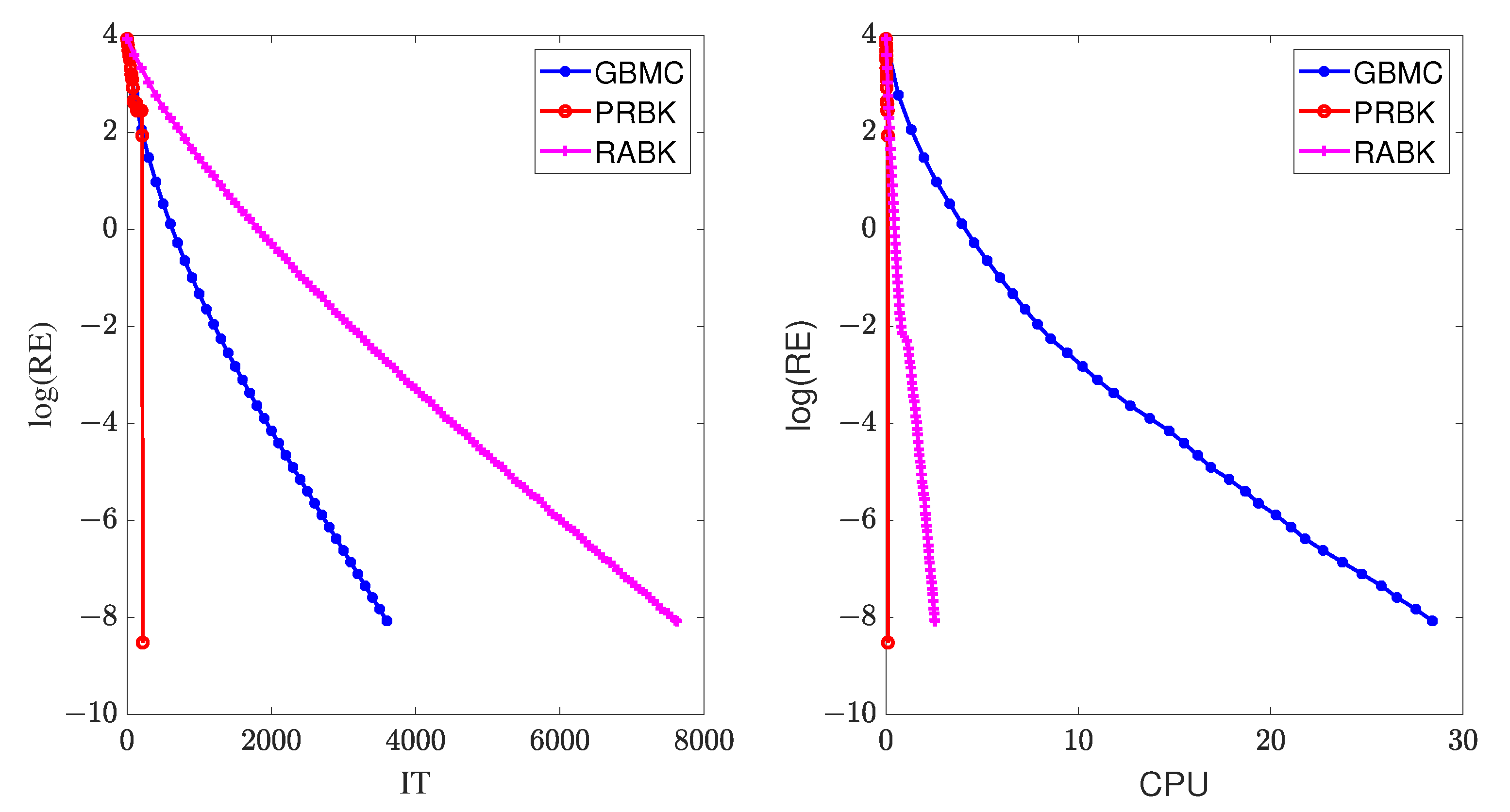
In this example, we set . The numerical results of IT and CPU are listed in Table 3 and Table 4, and the curves of relative error versus IT and CPU are drawn in Figure 4. From Table 3 and Table 4, we can observe that the MII-PRBK method has the least iteration steps and running time. The computational efficiency of the MII-PRBK and MII-RABK methods has been improved by at least 33 and 7 times compared to the GBMC method. Moreover, the advantages of the proposed methods are more pronounced when the matrix size increases.
Table 3.
The numerical results of IT and CPU for from Example 2.
Table 4.
The numerical results of IT and CPU for from Example 2.
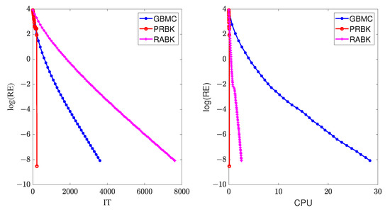
Figure 4.
The relative error of the different methods for from Example 2.
Example 3.
Consider dense Toeplitz matrices. For given , or .
In this example, we set . The numerical results of IT and CPU are listed in Table 5, and the curves of the relative error versus IT and CPU are drawn in Figure 5. We can observe the same phenomenon as that in Example 1.
Table 5.
The numerical results of IT and CPU for from Example 3.
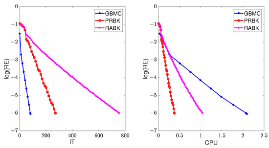
Figure 5.
The relative error of the different methods for .
Example 4.
Consider sparse Toeplitz matrices. For given , or .
In this example, we set . The numerical results of IT and CPU are listed in Table 6, and the curves of the relative error versus IT and CPU are drawn in Figure 6. Again, we can draw the same conclusion as that in Example 1.
Table 6.
The numerical results of IT and CPU for from Example 4.

Figure 6.
The relative error of the different methods for .
5. Conclusions
In this paper, we have proposed the randomized block Kaczmarz algorithms to compute inner inverses of any rectangle matrix, where A is full rank or rank deficient. Convergence results are provided to guarantee the convergence of the proposed methods theoretically. Numerical examples are given to illustrate the effectiveness. Since the proposed algorithms only require one row of A at each iteration without matrix–matrix product, they are suitable for the scenarios where the matrix A is too large to fit in memory or the matrix multiplication is considerably expensive. In addition, if the MII-RABK method is implemented in parallel, the running time will be greatly reduced. Therefore, in some practical applications, the MII-RABK method is more feasible when the Moore–Penrose generalized inverse is unknown or the calculation is too expensive. Due to limitations in hardware and personal research areas, we did not perform numerical experiments on very large-scale practical problems, which will become one of our future works. In addition, we will extend the Kaczmarz method to deal with the other generalized inverses of any rectangle matrix. Moreover, providing the feasible principles for selecting parameters and designing a randomized block Kaczmarz algorithm with an adaptive stepsize will be one of our future works.
Author Contributions
Conceptualization, L.X. and W.L.; methodology, L.X. and W.B.; validation, L.X. and W.B.; writing—original draft preparation, L.X.; writing—review and editing, L.X. and W.L.; software, L.X. and Y.L.; visualization, L.X. and Z.G. All authors have read and agreed to the published version of the manuscript.
Funding
This research received no external funding.
Data Availability Statement
The datasets that support the findings of this study are available from the corresponding author upon reasonable request.
Acknowledgments
The authors are thankful to the referees for their constructive comments and valuable suggestions, which have greatly improved the original manuscript of this paper.
Conflicts of Interest
The authors declare no conflicts of interest. The authors declare that they have no known competing financial interests or personal relationships that could have appeared to influence the work reported in this paper.
References
- Ben-Lsrael, A.; Greville, T.N.E. Generalized Inverses: Theory and Applications, 2nd ed.; Canadian Mathematical Society; Springer: NewYork, NY, USA, 2002. [Google Scholar]
- Cichocki, A.; Unbehauen, R. Neural Networks for Optimization and Signal Processing; John Wiley: West Sussex, UK, 1993. [Google Scholar]
- Guo, D.; Xu, F.; Yan, L. New pseudoinverse-based path-planning scheme with PID characteristic for redundant robot manipulators in the presence of noise. IEEE Trans. Control Syst. Technol. 2018, 26, 2008–2019. [Google Scholar] [CrossRef]
- Mihelj, M.; Munih, M.; Podobnik, J. Sensory fusion of magneto-inertial data sensory fusion based on Kinematic model with Jacobian weighted-left-pseudoinverse and Kalman-adaptive gains. IEEE Trans. Instrum. Meas. 2019, 68, 2610–2620. [Google Scholar] [CrossRef]
- Zhang, W.; Wu, J.; Yang, Y.; Akilan, T. Multimodel feature reinforcement framework using Moore-Penrose inverse for big data analysis. IEEE Trans. Neural Netw. Learn. Syst. 2021, 32, 5008–5021. [Google Scholar] [CrossRef] [PubMed]
- Zhuang, H.; Lin, Z.; Toh, K.A. Blockwise recursive Moore-Penrose inverse for network learning. IEEE Trans. Syst. Man, Cybern. Syst. 2022, 52, 3237–3250. [Google Scholar] [CrossRef]
- Sheng, X.; Wang, T. An iterative method to compute Moore-Penrose inverse based on gradient maximal convergence rate. Filomat 2013, 27, 1269–1276. [Google Scholar] [CrossRef]
- Wang, J. Recurrent neural networks for computing pseudoinverses of rank-deficientmatrices. SIAM J. Sci. Comput. 1997, 18, 1479–1493. [Google Scholar] [CrossRef]
- Wei, Y. Recurrent neural networks for computing weighted Moore-Penrose inverse. Appl. Math. Comput. 2000, 116, 279–287. [Google Scholar] [CrossRef]
- Wang, X.Z.; Ma, H.F.; Predrag, S.S. Nonlinearly activated recurrent neural network for computing the drazin inverse. Neural Process. Lett. 2017, 46, 195–217. [Google Scholar] [CrossRef]
- Zhang, N.M.; Zhang, T. Recurrent neural networks for computing the moore-penrose inverse with momentum learning. Chin. J. Electron. 2020, 28, 1039–1045. [Google Scholar] [CrossRef]
- Zhang, Y.; Guo, D.; Li, Z. Common nature of learning between backpropagation and Hopfield-type neural networks for generalized matrix inversion with simplified models. IEEE Trans. Neural Netw. Learn. Syst. 2013, 24, 579–592. [Google Scholar] [CrossRef]
- Stanimirovic, P.; Petkovic, M.; Gerontitis, D. Gradient neural network with nonlinear activation for computing inner inverses and the Drazin inverse. Neural Process Lett. 2018, 48, 109–133. [Google Scholar] [CrossRef]
- Lv, X.; Xiao, L.; Tan, Z.; Yang, Z.; Yuan, J. Improved gradient neural networks for solving Moore-Penrose inverse of full-rank matrix. Neural Process. Lett. 2019, 50, 1993–2005. [Google Scholar] [CrossRef]
- Zhang, Y.; Zhang, J.; Weng, J. Dynamic Moore-Penrose inversion with unknown derivatives: Gradient neural network approach. IEEE Trans. Neural Netw. Learn. Syst. 2022, 34, 10919–10929. [Google Scholar] [CrossRef] [PubMed]
- Ion, N. Faster randomized block kaczmarz algorithms. SIAM J. Matrix Anal. Appl. 2019, 40, 1425–1452. [Google Scholar]
- Xing, L.L.; Li, W.G.; Bao, W.D. Some results for Kaczmarz method to solve Sylvester matrix equations. J. Frankl. Inst. 2023, 360, 7457–7461. [Google Scholar]
- Du, K.; Ruan, C.C.; Sun, X.H. On the convergence of a randomized block coordinate descent algorithm for a matrix least squaress problem. Appl. Math. Lett. 2022, 124, 107689. [Google Scholar] [CrossRef]
- Du, K.; Si, W.T.; Sun, X.H. Randomized extended average block Kaczmarz for solving least squares. Siam. J. Sci. Comput. 2020, 42, A3541–A3559. [Google Scholar] [CrossRef]
- Strohmer, T.; Vershynin, R. A randomized Kaczmarz algorithm with exponential convergence. J. Fourier Anal. Appl. 2009, 15, 262–278. [Google Scholar] [CrossRef]
- Dax, A. Kaczmarz’s anomaly: A surprising feature of Kaczmarz’s method. Linear Algebra Appl. 2023, 662, 136–162. [Google Scholar] [CrossRef]

Disclaimer/Publisher’s Note: The statements, opinions and data contained in all publications are solely those of the individual author(s) and contributor(s) and not of MDPI and/or the editor(s). MDPI and/or the editor(s) disclaim responsibility for any injury to people or property resulting from any ideas, methods, instructions or products referred to in the content. |
© 2024 by the authors. Licensee MDPI, Basel, Switzerland. This article is an open access article distributed under the terms and conditions of the Creative Commons Attribution (CC BY) license (https://creativecommons.org/licenses/by/4.0/).