Analysis of Production and Failure Data in Automotive: From Raw Data to Predictive Modeling and Spare Parts

Abstract

The present analysis examines extensive and consistent data from automotive production and service to assess reliability and predict failures in the case of an engine control device. It is based on statistical evaluation of production and lead times to determine vehicle sales. Mileages are integrated to establish the age of the vehicle fleet over time and to predict the censored data. Failure and censored times are merged in a multiple censored data and combined by the Kaplan-Meier estimator for survivals. The Weibull distribution is used as parametric reliability model and its parameters identified to assure precision in predictions (>95%). An average time to failure >80 years and a slightly increasing failure rate ensure a low risk. The study is based on real-world data from various sources, acknowledging that the data are not homogeneous, and it offers a comprehensive roadmap for processing this diverse raw data and evolving it into sophisticated predictive models. Furthermore, it provides insights from various perspectives, including those of the Original Equipment Manufacturer, Car Manufacturer, and Users.

1. Introduction

The rapid advancement of technology, the development of highly sophisticated products, strong global competition, and increased customer expectations have put new pressure on manufacturers to ensure increasingly high-quality products [1,2,3]. Customers expect the products they purchase to be reliable and safe. We are all aware of the need for a product to be reliable; however, when we try to quantify this characteristic, the process proves to be far from simple [4,5,6].

Carrying out a reliability study starting from the observation of the failure data of components subjected to real conditions of use [7,8,9] consists of:

• collect and record information on failures and defects found.
• filter, interpret and analyze all this information.
• obtain the probability curves that represent the reliability behavior of the product.
• predict the trend of future failures over time.

This procedure, known as Reliability Data Analysis (RDA), can affect the major industrial sectors, but is particularly effective where high production and very strong product quality requirements coexist, as in the case of the automotive.

Numerous valid studies attempted to derive the reliability of vehicles or their parts [10,11,12,13], so much so that the techniques used are rather consolidated nowadays [14,15,16]. The present report aims to add its contribution by describing in full detail an analysis carried out on a real case series.

The paper presents a detailed approach for assessing and predicting the reliability of automotive parts using a variety of data by the following sections.

• Materials and Methods: The research begins by gathering and examining data from an automotive Original Equipment Manufacturer (OEM) and a Car Manufacturer (CM). This includes data on original and spare part production, lead times, and vehicle mileage. The study also pays close attention to how data on part failures is collected and analyzed. For estimating the reliability of automotive parts, the study first uses the Kaplan-Meier estimator, a non-parametric method. Then, it shifts to the Weibull model, a parametric method, for predicting when parts might fail over time.
• Results and Discussion: The paper discusses the main outcomes. This includes determining when parts start being used, how the vehicle fleet ages over time, and both non-parametric and parametric estimates of part reliability. It also explores forecasting the need for spare parts and examines how well the methodology works. It also concludes that its approach effectively combines different types of data to predict when automotive parts might fail. The predictions match well with the actual data, although the paper notes some factors that might explain any small differences.

Although failure data analysis is a well-explored field with a multitude of studies, this work distinguishes itself by adeptly merging various elements such as:

• Comprehensive Data Integration: it integrates data from various sources in the automotive sector, including original and spare part production, vehicle mileage, and failure data. This multi-faceted approach is relatively unique.
• Advanced Statistical Techniques: The use of both non-parametric (Kaplan-Meier estimator) and parametric (Weibull distribution) methods for predicting failures represents an advanced statistical approach, especially outside the use of software tools. This dual method enhances the accuracy and reliability of predictions.
• Real-World Application and Validation: The study is grounded in real-world data, also in the sense that the data are not filtered or corrected to simplify the analysis. This aspect adds significant value to the research, as it demonstrates the applicability of the findings in actual industrial scenarios.
• Methodological Framework: The research outlines a detailed methodological framework that can be replicated or adapted for similar studies in other contexts, making it a valuable reference for future research in the field.
• Multi-Dimensional Analysis: The analysis considers various factors like lead time, production trends, and vehicle usage patterns. This holistic view is relatively novel in automotive reliability research, which often focuses on narrower aspects.
• Consideration of Censored Data: The paper’s approach to handling censored data (by simulating them) in the analysis is methodologically sound and enhances the robustness of the study’s conclusions.
• High Precision in Predictions: The study achieves high precision in its predictive models (over 95% accuracy), which is notable in the field of reliability engineering.

These elements collectively showcase the paper’s contribution to the field of automotive reliability and predictive modeling, demonstrating a blend of theoretical innovation and practical application.

2. Materials and Methods

2.1. Production and Use

The current case study, derived from a significant industrial context, consists of a Reliability Data Analysis (RDA) focusing on a component of an Engine Control System.

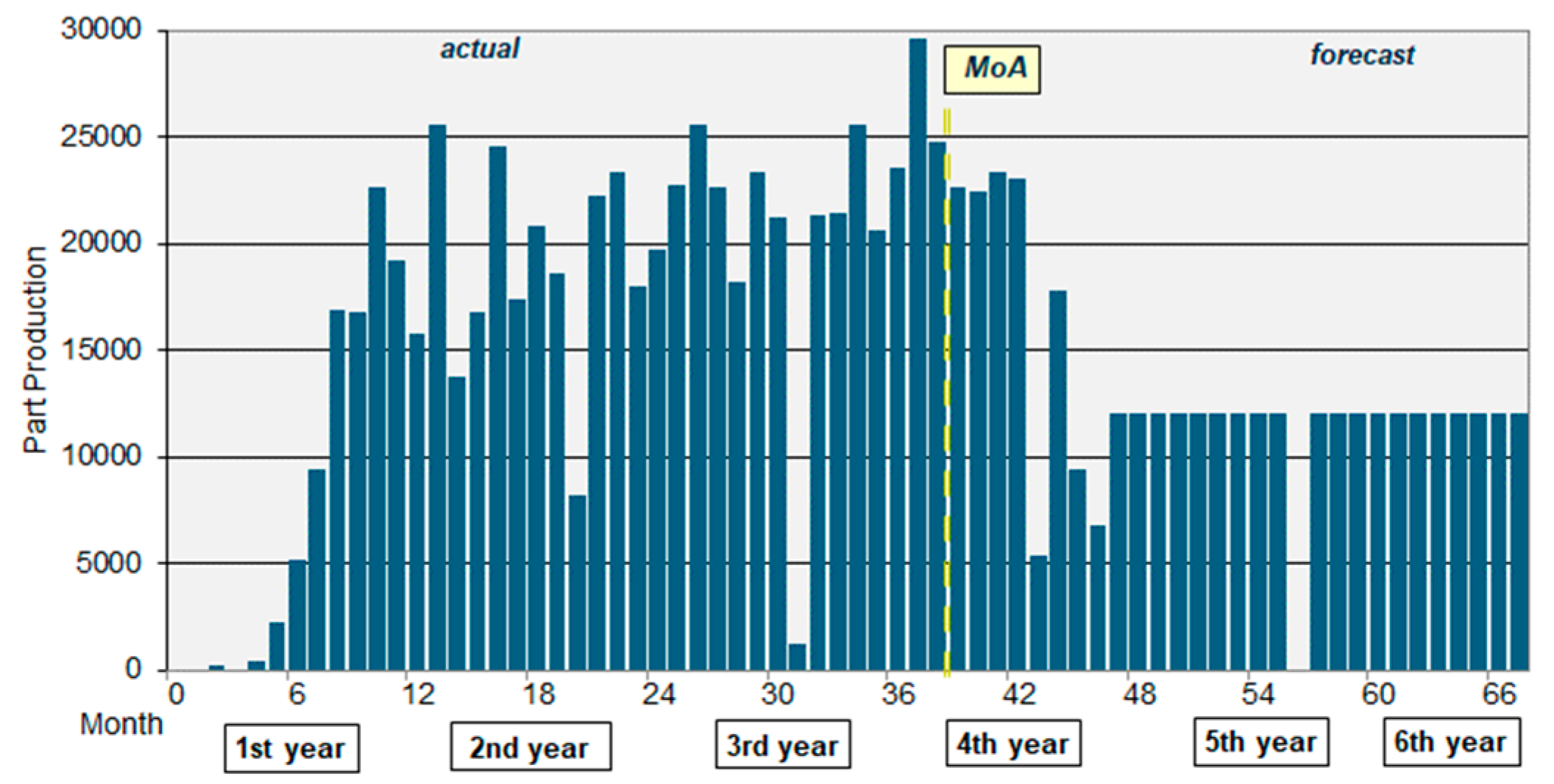
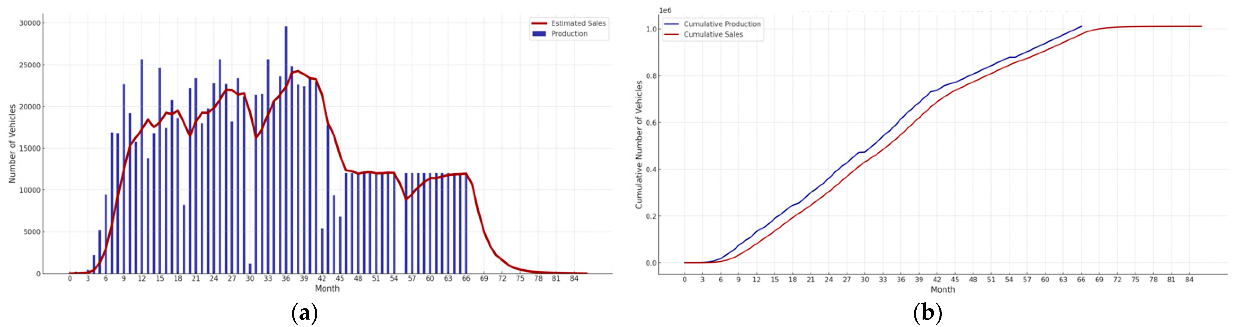
2.1.1. Original Part Production

The production order, containing 1.1 million components, is expected to be fulfilled by the Original Equipment Manufacturer (OEM) in approx. 5.5 years (~66 months). Figure 1 displays the monthly production over the time, as derived by a precise policy of production optimization, coupled with a process flexibility that allow production to be fractionated inside a “lean pull” logic. It is characterized by:

• an ‘acceleration ramp’ increasing the production rate to 20,000 parts/mo. in ½ year.
• the saved possibility to boost (by +50%) productive targets, whenever necessary.
• a large variability, ranging from a few parts (in August) to 30,000 units/month.
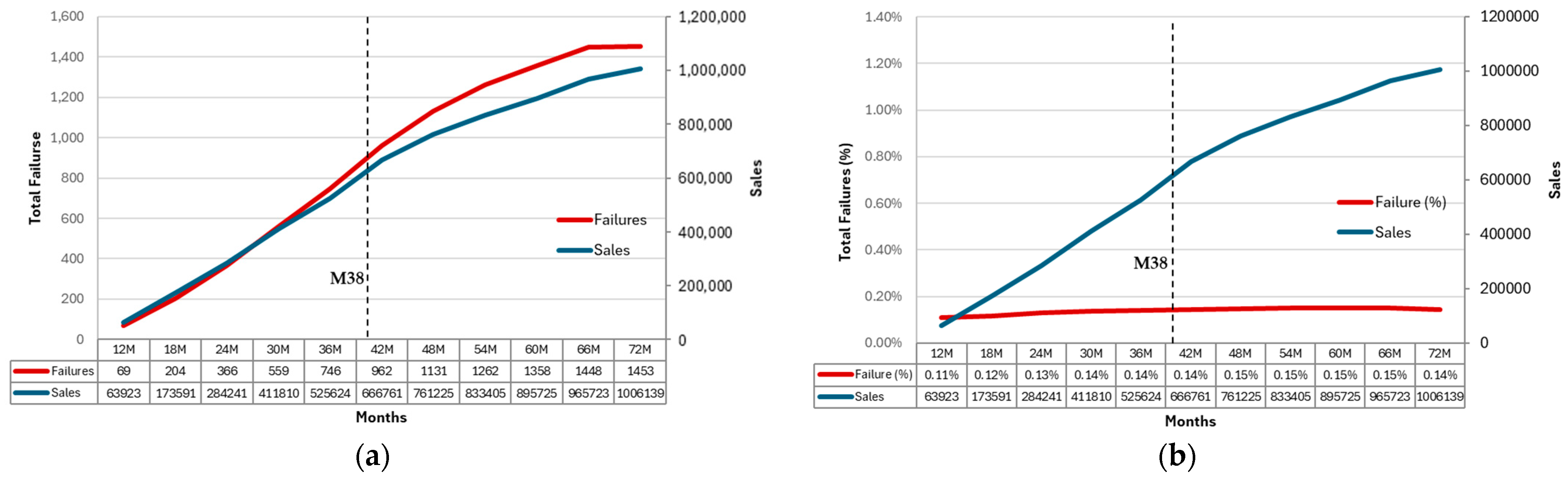
• 64% of production completed at the Moment of the Analysis (MoA) = 38th month (M38)
• a production trend precisely known only up to a few months beyond this limit (M38)

The successive production is constant as it is not yet been optimized, simply expressed as an average production value, able to meet the entire order.

This trend represents the starting point of the investigation.

2.1.2. Spare Part Production

Data on the spare part production over the time, up to the MoA, is also available, and shown in Figure 2, underlining that:

• the spare part production starts late respect to the original part production considering that spare part need is low as long as the vehicles have come a short distance.
• the alignment between original part and spare part productions happens gradually.
• in the meantime, it is possible to establish an initial stockpile (of spare parts) by leveraging those (limited) overproduction situations typical of production processes.

The Figure 2 also highlights no detailed information is currently available for a significant period following the MoA (=38M), even if the ability to accurately predict the failure number over time (i.e., over 6 years) can represent an operational advantage for the OEM: it manages to anticipate the demand for spare parts (e.g., by optimizing production, warehouse, logistics and distribution in the territory, etc.), as well as budgeting for the correct warranty costs. This estimation can have a further important impact: if, as in the present case, the production systems are slated for reconfiguration upon order completion, it becomes essential to generate an adequate stock of spare part, able to respond to customer requests (withing 10 years, at least, as a legal constraint).

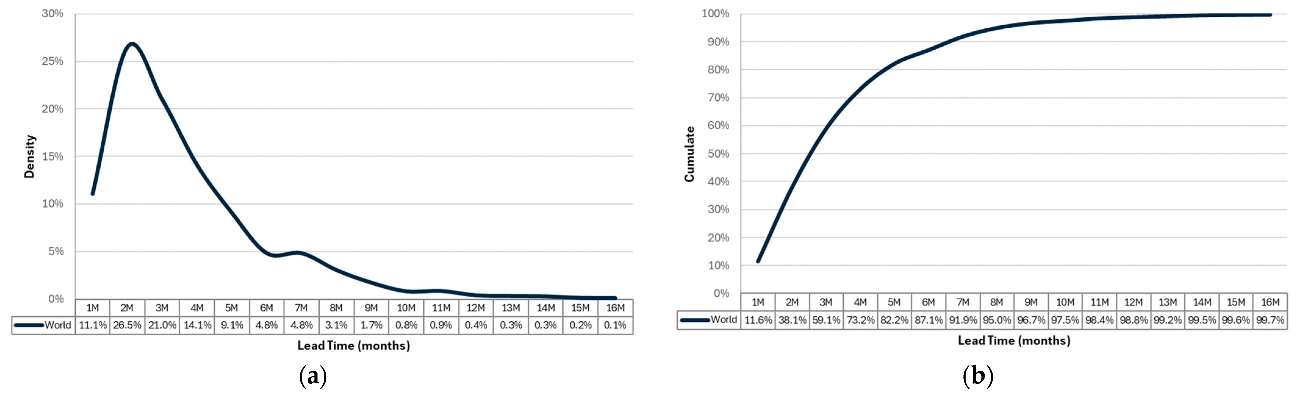
2.1.3. Lead Time

Once produced (by OEM), the part is delivered to Car Manufacturer (CM), installed in the vehicle, introduced to the market, and purchased by the end user, also representing the moment from which the system begins to operate. In this context, lead time (LT) is defined as the time interval from when a system is produced to when it becomes operational. Its determination is a complex task: it involves a mix of non-homogeneous factors (e.g., geographical peculiarities, market trends, presence of sales policies, logistics, etc.).

Furthermore, neither the OEM nor the CM can derive this knowledge independently, and the best way to determine the LT in the present situation is to derive it directly from the available data. For the scope, a stochastic sample, consisting of records from 2633 vehicles, is extracted and analyzed.

Figure 3 shows this lead time (in months) in terms of Probability Density Function (PDF) and Cumulate Distribution Function (CDF). Although they are here represented as continuous curves, data is available in the form of histograms of frequencies and cumulates. For instance, the PDF first value (Figure 3a), equal to 11.1%, represents the probability that the part enters service within a month (i.e., 15 days) from production. The most frequent value (namely, the mode), at 26.5% of frequency, occurs at the 2nd point and a DL between 1 and 2 months (i.e., 45 days). Similarly, the CDF second point, equal to 11.6%, represents the probability that the LT is ≤2 mo. (avg. 45 days) and, consequently, 88.4% is the probability that LT is >2 months. Considering the CDF at 50%, it is possible to state that approximately half of parts enters in service within 3 mo., 85% within 6 months and almost all within one year.

The information is essential for failure predictions.

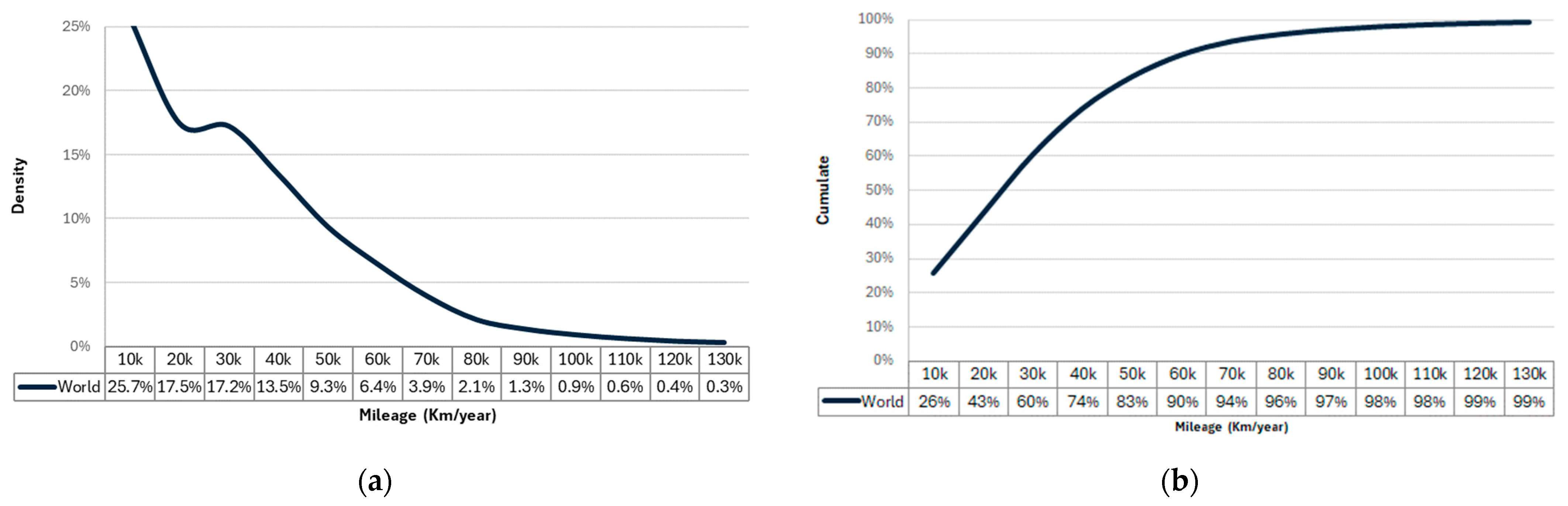
2.1.4. Mileage

Once the vehicle is in service, everyone drives it as they prefer. However, thanks to the fact that vehicles undergo maintenance from time to time (e.g., routine services) car manufacturers can easily record accurate information on the mileage traveled by their customers, respect to each specific vehicle, motorization, market, etc.

In the present case, the mileage, expressed in km/year, is reported in Figure 4, as Probability Density Function (PDF) and Cumulate Distribution Function (CDF). A relevant decrease is visible in the PDF, as the mileage increases, with, e.g., 25.6% users driving less 10,000 km/year, 17.2% between 10,000 and 20,000 km/y. From the CDF, it similarly emerges 60% of users drives less than 40,000, 90% run 70,000 and only 3% passes the 100,000 km/y. These cars, belonging to the D- and E-segments, have an annual mileage estimated as 28,450 km on average and ~20,000 km as median.

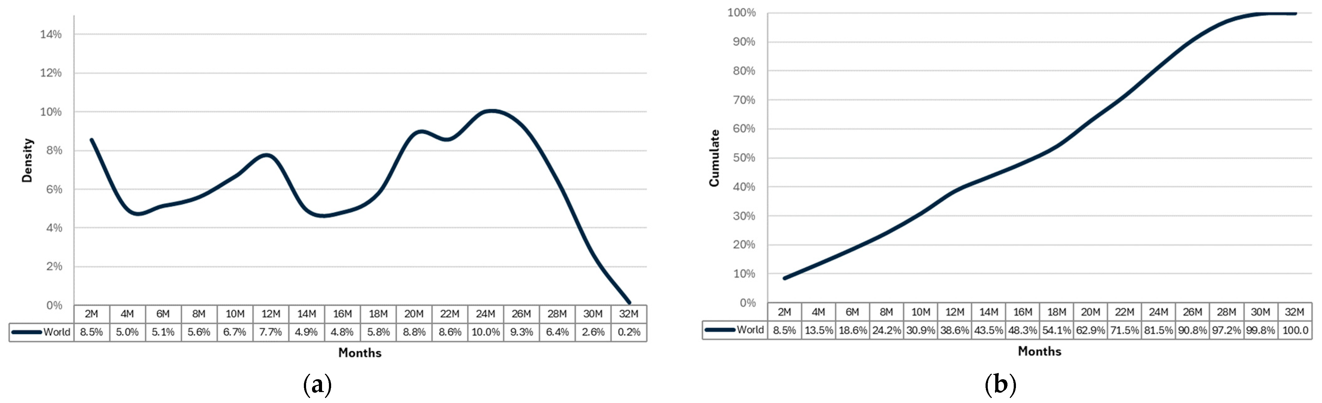
2.2. Failure Data

Failures are usually reported to the Car Manufacturer through the assistance service. In the present case, 2675 failures are available, each one providing information such as:

• Chassis number.
• Assembly date.
• Delivery date.
• Claim date.
• Country.
• Age in month.
• Mileage.

The following Figure 5 and Figure 6 show the failure distribution respect to mileage (in km) and time of use (in month), respectively.

From this perspective, it is relevant to highlight that:

• both metrics can conveniently serve for assessing the system reliability. The choice between them depends on the specific nature of the failure under investigation. In this study, given that the failure is related to engine control components, the mileage is chosen as metric for analysis (‘running unit’), as more pertinent for the case.
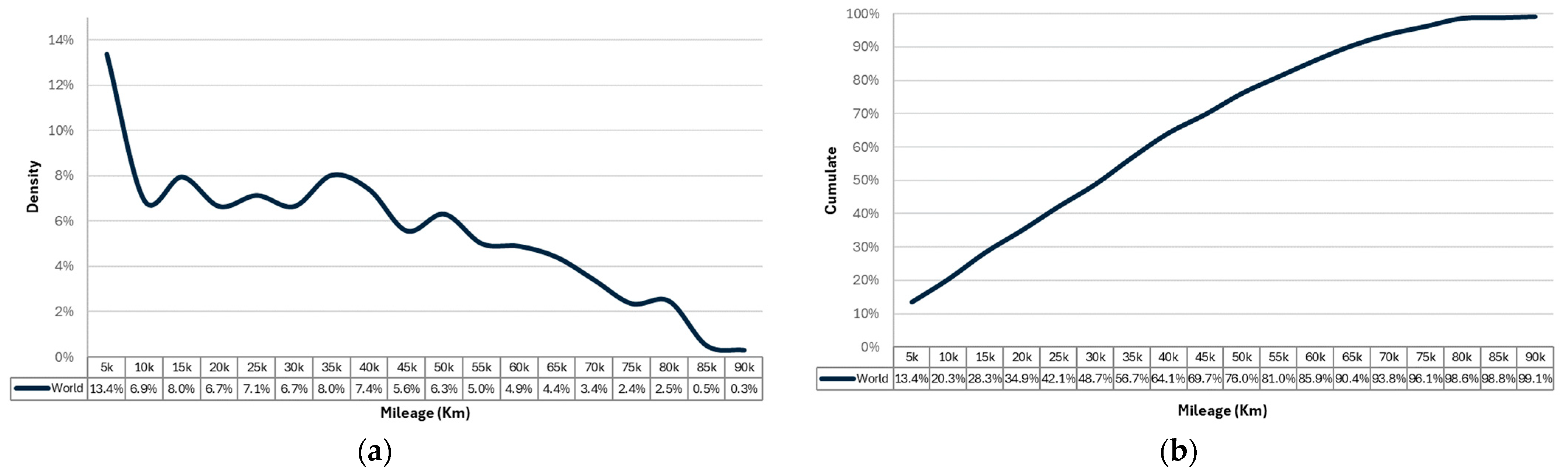
• while the diagrams in Figure 5 and Figure 6 can be used for a preliminary overlook about what is happening in the circulating fleet of cars, they are not able to characterize the reliability behavior as they fail to incorporate essential information such as the “fleet mileage aging”. For instance, Figure 5a highlights 8% of failures between 30,000 and 35,000 km, but it misses to clarify how many cars ended up traveling these mileages.
• more generally, to correctly evaluate the reliability behavior, it is necessary to incorporate the “censored times”, i.e., survival data, which indicate that certain parts have endured certain operating times. And a simulation is needed for the scope.

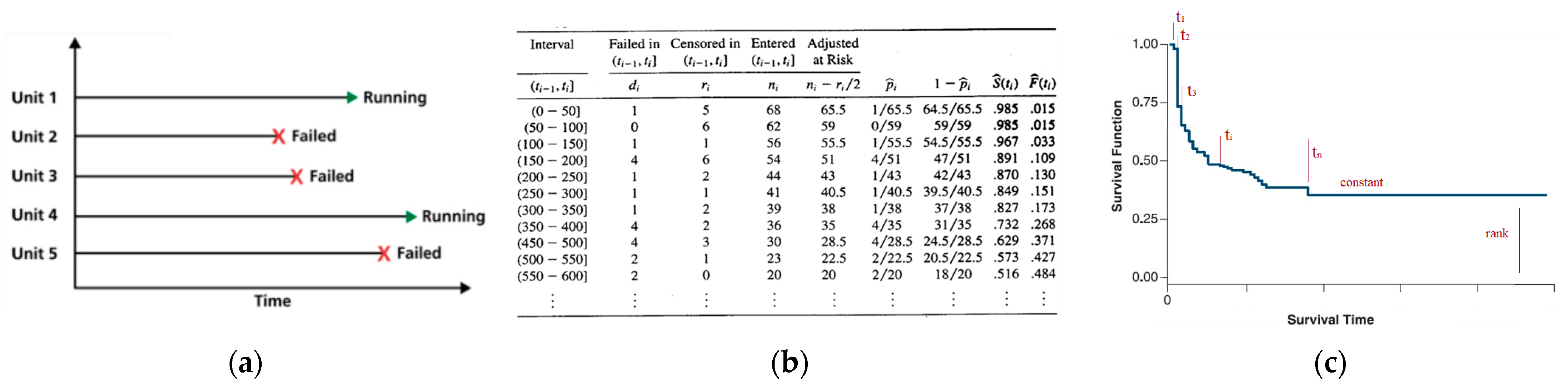
2.3. Survival Non-Parametric Estimation

The censored data represents information that can be collected from the data system, distinct from direct failure data. When analyzing the data at a specific Moment of the Analysis (i.e., M38), determined by the most recent update of failure data (i.e., 2675 parts failed), all parts that have not failed during the same period (i.e., “running”) must also be considered in the calculation. They provide “positive information” regarding the system reliability, in contrast with the “negative information” derived from failures. Moreover, the value of this positive information grows with the parts’ age—the longer they have operated without failures, the more they can be considered reliable. Then, the scenario requires not only identifying censored parts but also evaluating their aging, in what is commonly known as “multiple censoring data”, as represented in Figure 7a. This system can be effectively analyzed offering a comprehensive understanding of component reliability over time.

Specifically, the Kaplan-Meier estimator is here used for the scope (as in [17]) which allows to calculate the survival function (S_i). This estimator is part of a well-known procedure for reliability estimation involving the definition, for a given period, of a group of parts that are at risk of failure (“risk set”) as a mean to appropriately weigh the failures have occurred. Through this ratio, it is possible to determine the probability of survival for a given period, and then proceed further. By multiplying these probabilities, the survival function can be established which aims to derive the non-parametric estimator of reliability and then, the unreliability.

Figure 7b presents the Kaplan-Meier procedure, for evaluating the survival probabilities over time. It accounts for both failure and censored data and involves:

• Time interval (t_i − t_i−1), the period (e.g., hours, km, …) over which the data is observed.
• Failed in Interval (di), the number of failures that occurred during each time interval.
• Censored in Interval (r_i), the number of censored data points in each time interval, representing units that have not failed but are no longer being observed.
• Entered (n_i), the ‘risk set’, equal to the total number of subjects at risk of failure (‘at-risk’) at the beginning of each time i interval.
• Adjusted At Risk (2n_i − r_i/2), an adjustment to the at-risk number (n_i) to better account for censored cases and better reflect the average risk during the interval.
• Failure Risk (p_i), the probability of failing through the end of the i interval, calculated as the number of failed (d_i) by the adjusted number at risk (2n_i − r_i/2).
• Survival Probability (1 − p_i), the probability of surviving without failure through the end of the i interval.
• Survival Function (S(t_i)), the product of all previous interval survival probabilities (1 − p_i), representing the overall survival probability up to that point in time t_i.
• Failure Function (F(t_i)), the probability that failure has occurred by time t_i, which can be calculated as 1 − S(t_i).

The Kaplan-Meier estimator is called non-parametric method in the meaning it does not suppose any specific distribution for survival times [17]. It simply presents an empirical survival function that can be applied to estimate the survival probability at any given failure time. However, it cannot provide estimates beyond the highest failure time. This is represented in Figure 7c, where, starting from the highest failure time (i.e., t_n), the survival function remains constant (at a value called ‘rank’). But this contradicts the reality which presupposes that the probability of survival always decreases to 0 for $t\to \infty$.

Then, it is essential to transition from a non-parametric estimator (i.e., Kaplan-Meier estimator) to a parametric estimator through analytical methods, able to determine mathematical models behind data distributions.

2.4. Weibull Reliability Function

The Weibull distribution is here used for the scope. It is a continuous probability distribution named after Wallodi Weibull, who described it in detail in 1951 [18], although it is originally identified by Fréchet in 1927 [19]. It is particularly suited to representing the life of manufactured products, characterizing life data with its flexibility to model various types of behaviors. This happens because, in fact, the formulation proposed by the Weibull model is the one that mathematically represents the very common case in engineering of a complex system that fails as soon as one of its subsystems fails. As it is formulated, it is also very flexible, managing to approximate the behavior of failure data well in very different situations (early failures, aging, etc.), often making this model the best solution for a reliability study.

Here, after having hypothesized the Weibull model could properly represent the data system (as in similar investigations [20,21,22,23]), such model is used to predict failures over time. For the scope, the linearization offered by a Weibull plot permits to detect the proper model parameters ([24]).

A Weibull plot is a graphical method used in statistical analysis to assess the distribution of a dataset, largely accepted for modelling time-to-failure data in reliability engineering. The Weibull distribution is characterized by two parameters: the shape parameter (k), which indicates the failure rate over time, and the scale parameter (λ), which indicates the characteristic life (the time by which 63.2% of the population will have failed).

In a Weibull plot, times-to-failure data points are plotted on a graph with both axes typically on a logarithmic scale so that if the data follows a Weibull distribution, it will appear as a straight line, indicating linearization of the data. Moreover, the same Weibull plot can be used to derive the line (and consequently, the specific Weibull model) that best approximates the dataset, by determining the two Weibull parameters of shape and scale.

Then, by analyzing the linearity of the data in a Weibull plot, it is possible to:

• infer the reliability and failure behavior of products or systems,
• estimate their lifetime,
• make decisions about maintenance and warranty.

The simplified approach of using a Weibull plot, instead of more advanced statistics tools (able to automatically compare different parametric estimators and failure models), is here preferred to better discuss the intermediate steps of the procedure.

2.5. Methodological Framework

The present RDA is based on the following aspects:

1.

Input Data

a.

Production Trend (from the OEM database)

b.

Lead Time Distribution (from the OEM database and CM market data)

c.

Mileage Distribution (from CM service data)

d.

Failure Data (from CM service data)

2.

Derived Data

e.

Sales Trend (combining Production and Lead Time)

f.

Fleet Mileage Aging (combining Delivery and Mileages Distribution)

g.

Censors (considering the Fleet Mileage Aging at the MoA)

h.

Multiple-Censoring Failure Dataset

i.

Reliability Non-Parametric Estimation (by Kaplan-Meier Estimator).

j.

Reliability Parametric Estimation (by Weibull failure model)

k.

Spare Parts Prediction (from Fleet Mileage and Reliability Estimation)

Figure 8 incorporates these elements into a workflow, highlighting their connections. In particular, the input data are distinguished from those derived analytically, and it is also indicated what information is available in the form of datasets or distributions.

Specifically, the following steps can be used to summarize the procedure:

• Production Trend and Lead Time Distribution are combined to obtain the Sales Trend which effectively estimates the moment in which the vehicles entered the operational state and begin to accumulate kilometers. After this, Production Trend and Lead Time Distribution are no longer needed, replaced in subsequent calculations by the Sales Trend.
• Sales Trend and Mileage Distribution are combined to obtain the Fleet Mileage Aging, identified as the distribution of kilometers traveled by vehicles in circulation. This distribution changes over time, moving to ever higher mileages, and is calculated at different times for different scopes.
• As first, the Fleet Mileage Aging is evaluated respect to the exact moment the failure data are updated (MoA). Thus, it is determined the mileage distribution of the vehicles put into circulation, representative of the failures recorded. This distribution allows us to identify the censoring data.
• Failures and censorship data are combined to obtain a multiply censored data from which it is possible to evaluate a (non-parametric) estimation of the reliability/survival function by applying the Kaplan-Meier method.
• This initial (non-parametric) estimation is improved using a Weibull model, deriving an analytical formulation for the reliability behavior of the system. The Weibull model is parametric, i.e., it changes shape as the parameters change. In the specific case, the two (shape and scale) parameters are determined to best approximate the values obtained from the (non-parametric) Kaplan-Meier estimator. However, it is worth clarifying the following. Among various potential models (e.g., Exponential, Lognormal), the Weibull model is selected a priori due to its general characteristics, such as flexibility, making it particularly suitable for our purpose. Typically, multiple models are hypothesized and the best fit for the data is chosen. However, in this specific case, the precision achieved with the Weibull model is so high that further refinements are deemed unnecessary.
• Given the reliability function, the Fleet Mileage Aging calculation comes in handy again. For each time of interest (e.g., every 12 calendar months), in fact, the related Fleet Mileage Aging is combined with the Reliability to determine the number of failures that occurred by that date. This provides a tool that allows to evaluate the spare part request month by month.

The validation of the procedure can take place by checking at any time the correspondence between the number of expected and occurring breakages. However, as discussed below, this is not straightforward in practice and, therefore we are forced to accept only a partial verification of the predictive technique.

3. Results and Discussion

3.1. In Operation

The first step is to estimate when the parts (Figure 1) are expected to come into operation due to the presence of the lead time (Figure 3). This preliminary task is required due to limited access to sales data, exclusive to the Car Manufacturer. For the scope, a Monte Carlo extraction procedure permits to combine the two phenomena (production trend and lean time distribution), computing at the estimated sales distribution at M38. In Figure 9, it is possible to see a direct comparison between the trends, noting that:

• the application of a lead time (LT) smooths distribution the sales trend.
• their cumulative trends run parallel, with a minimal shift (approx. 1 month).

3.2. Fleet Aging

The second step aims to estimate the censored data and their mileages (‘fleet aging’) at the Moment of Analysis (M38). Their number is equivalent to the CDF of the Estimated Monthly Sales after 38 months, equal to 572,025. A new Monte Carlo extraction procedure makes it possible to combine the Sales Trend over time (Figure 9) and the distribution of mileage in km/year (Figure 4), providing the ‘fleet mileage aging’ shown in Figure 10 in terms of density (PDF) and cumulate functions (CDF). For instance, the first value of PDF in Figure 10a evaluated that 21.0% of vehicles have traveled less than 10,000 km, 19.3% between 10,000 and 20,000 km, and only 0.6% between 150,000 and 160,000 km. The CDF in Figure 10b reports, e.g., that 91.8% of vehicles have travelled less than 100,000 km and no one has exceeded 210,000 km so far. To refer to the real values, it is sufficient to consider that, as said, the M38 are delivered 572,025 vehicles (see Figure 9b).

Thanks to the evaluation of the fleet aging at 38M, it is trivial to estimate travel distances of the censored vehicles since the two aspects mostly coincide. Then, it can be said that, e.g., 21.0% of 572,025 vehicles (=171,608) are censored between 0 and 10,000 km (=5,000 km as average) or 0.6% (=34,322) between 150,000 and 160,000 km (=155,000 km).

Combining failure and censored data, the multiply censored system is established, as represented in Figure 11. It is immediately manifest the reduced number of failures, lower than 1% respect to the total vehicles, and their main impact around 30,000–80,000 km.

3.3. Non-Parametric Estimation

The Kaplan-Meier method considered 2675 failures and 569,446 censored data, with the procedure represented in Figure 12. A truncation of ~0.45% (equivalent to 2579 censored data) is applied eliminating the entire upper tail of the distribution (>250,000 km) with the scope to address potential issues with the consistency of information in these higher mileage cases.

It can be observed, then, the initial risk set of 569,446 (n_i) entering in the 1st interval (0–5,000 km) of risk where 358 vehicles failed (d_i) while 59,595 vehicles (r_i) are censored. According to the procedure, the entered risk set is adjusted reducing its value for half of the number of censored data (n_i − r_i/2), before using it in the survival evaluation. Specifically, the risk of failure occurring precisely in that i-interval (p_i) is equal to the ratio between the failures (d_i) and the adjusted risk set (n_i − r_i/2). Consequently, as the complement to 1, it is possible to calculate the probability of exceeding the interval without failures (1 − p_i), while the survival function at that i-interval (S_i) is equal to the probability of having exceeded each of the previous intervals, which is obtained by multiplying this probability (1 − p_i). The probability of failing (F_i), equal to the probability of not surviving is obtained as the difference with 1 of the probability of surviving.

The Kaplan-Meier reliability and unreliability estimations are shown in Figure 13. Reliability begins (as expected) at 100%, decreasing to 98.8% within the first 80,000 km, after which the rate of decline slows down. Unreliability follows a corresponding pattern.

Moreover, no estimate is available much beyond 100,000 km because no failure has occurred so far. The presence of censor data at higher values (i.e., ~41,000 censored data over 100,000 km) affects the trend without allowing to extend it. As said, in fact, in the case of non-parametric estimators, only failures allow the reliability to be fully defined. To make predictions beyond this limit, a parametric estimator is needed.

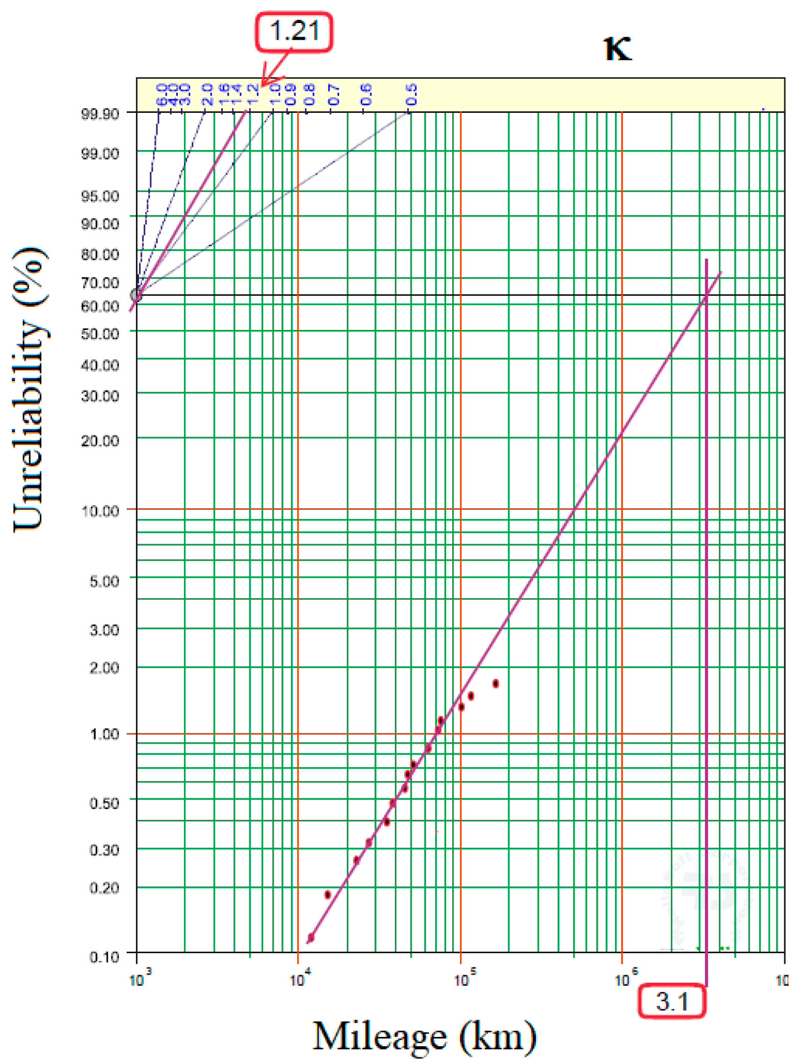
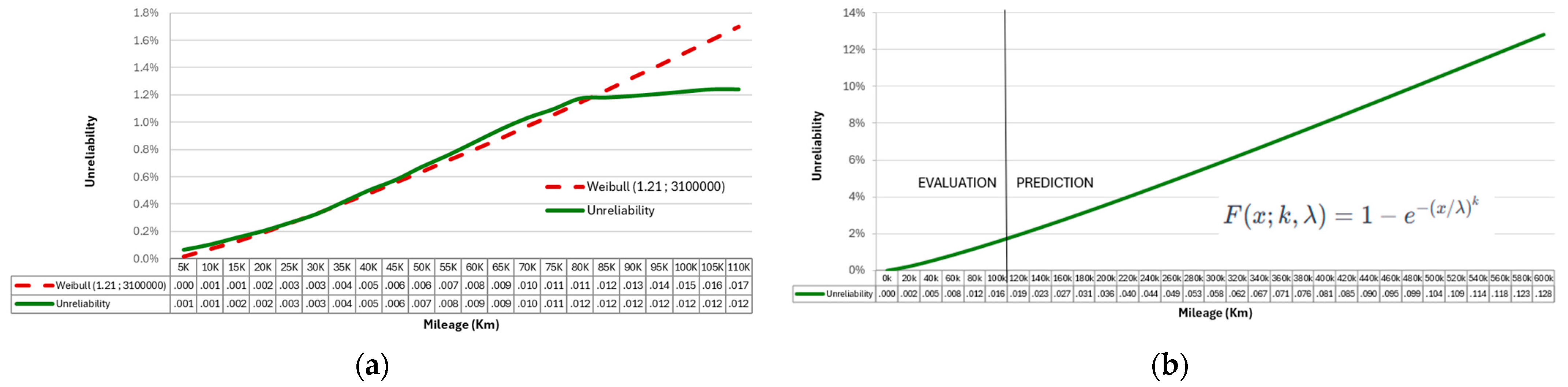
3.4. Parametric Estimation

Data is analyzed by a Weibull failure model and a ‘best fit’ approach over a Weibull plot. The goal is to ensure that the model closely matches the pattern of the actual failures observed in the data. This means that the line that best approximates the failure times as represented on the Weibull Plot must be found. Figure 14 shows the use of a Weibull Plot. Data is reported by the logarithmic scales for X-axis (Mileage in km), representing the time until failures, and a Y-axis (Unreliability %) with the probability of failure (unreliability) in percentage. This probability is typically plotted on a nonlinear scale that makes data appears as a straight line when follows a Weibull distribution.

The diagonal line represents the line of best fit of the plotted values: from its inclination, the shape parameter is derived (k = 1.21), and from its intersection with the value of F = 63.2%, the scale parameter (λ = 3.1 × 10⁶) is obtained. The reason why such value is used in the context of the Weibull distribution is related to the definition of the scale parameter: it represents the time-to-failure value at which the probability of failure is approx. 63.2% regardless for the specific shape of the model. Then, it serves as a useful reference point in Weibull distribution analysis for reliability and failure prediction purposes. The line that intersects at approximately 63.2% on the Weibull Plot is the scale line, and this intersection is used to determine the value of the scale parameter.

Finally, the procedure permitted optimizing the model by error minimization, based on the hypothesis that the Weibull model accurately represents reliability behavior. The fact that the points are effectively distributed along a straight line confirms the hypothesis.

In Figure 15a the unreliability predictions in the cases of non-parametric estimator (via Kaplan-Meier) and parametric estimator (via Weibull) are compared: the differences are marginal for most of the range (i.e., 4–5% as average gap and 97.5% as correlation coefficient). Regarding the region where such difference is not negligible (>75,000 km), it should be considered that the non-parametric estimation is generated based on a relatively small dataset (=38 failures) and, therefore, its precision may be limited. Moreover, the steep decline in climbing speed, as seen in Figure 15b, lacks a meaningful physical interpretation. This figure underscores a key motivation for turning to parametric analysis: the ability to extrapolate reliability behavior beyond failure times, enabling accurate predictions.

3.5. Failure Model

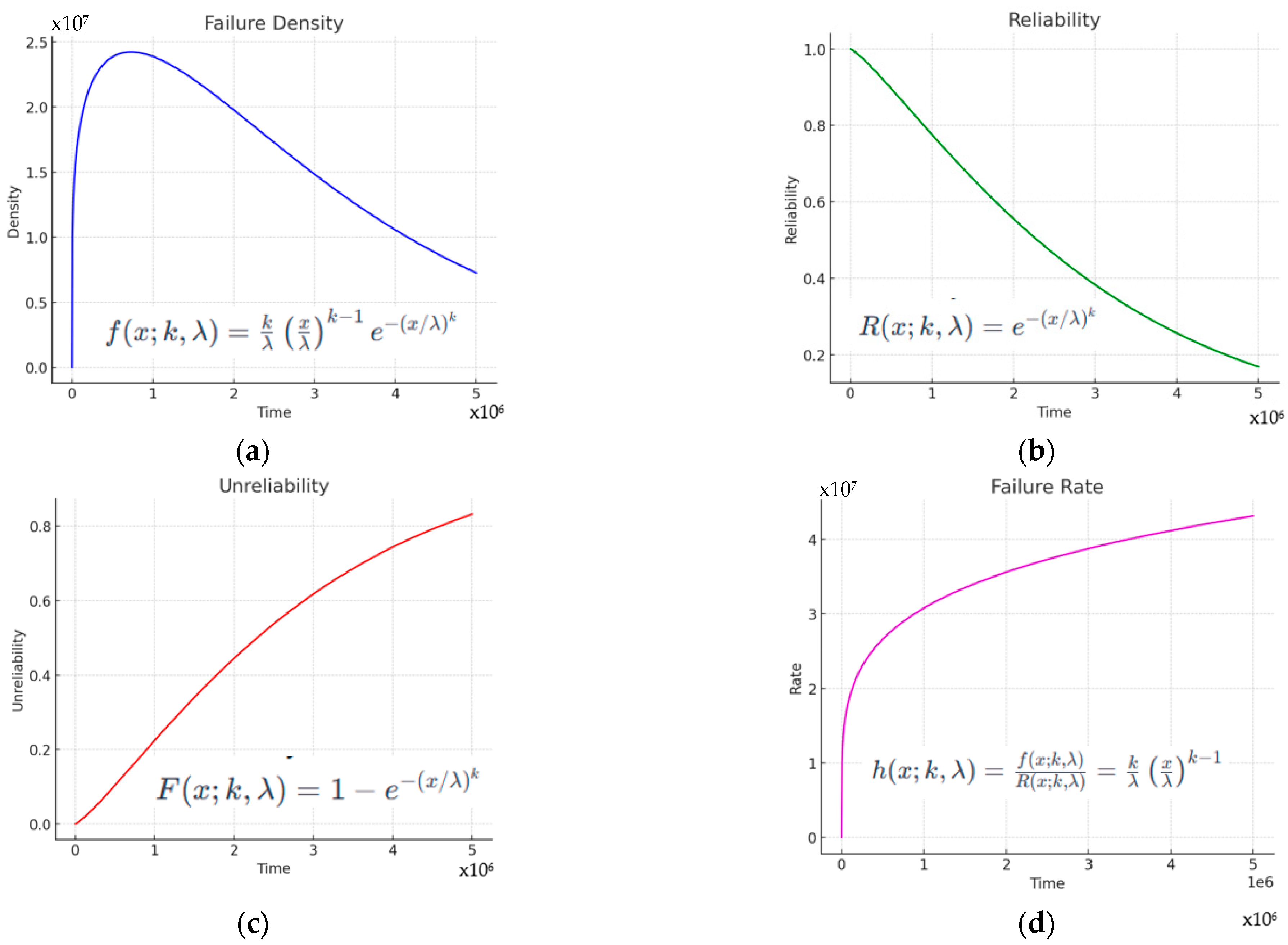
Specifically, the RDA permitted to the identify the following failure model,

$$f\left(x;k; \lambda \right)=\frac{k}{\lambda }{\left(\frac{x}{\lambda }\right)}^{k-1}{e}^{-{\left(x/\lambda \right)}^k}, \text{as failure density (PFD)},$$

(1)

$$F\left(x;k; \lambda \right)=1-e^{-{\left(x/\lambda \right)}^k}, \text{as unreliability function (CDF)},$$

(2)

$$R\left(x;k; \lambda \right)=e^{-{\left(x/\lambda \right)}^k}, \mathrm{as} \mathrm{reliability} \mathrm{function}$$

(3)

$$h\left(x;k; \lambda \right)=\frac{k}{\lambda }{\left(\frac{x}{\lambda }\right)}^{k-1}, \mathrm{as} \mathrm{failure} \left(\mathrm{hazard}\right) \mathrm{rate}$$

(4)

when the two parameters of shape, k = 2.1, and scale, λ = 3,100,000 are used (Figure 16).

As known, F(x) is the cumulate probability that a failure occurs within a certain mileage (x); R(x) is similarly the probability that this failure does not occurs, while h(x), the hazard rate, is the instantaneous probability of failure per unit of mileage given that no failure has occurred up to that point.

Considering the trends, it can be said that:

• Failure density shows that the failure probability density starts at zero, increases until it reaches a peak, and then gradually decreases. The peak indicates the point where a failure is most likely to occur. The shape of the graph reflects the fact that with a form factor greater than 1 (1.21 in this case), failures tend to increase with time, suggesting a wear or aging effect.
• Reliability, as expected, starts at 1 (100% reliability) and decreases over time. The curve shows a relatively gradual decrease in reliability, indicating that the probability of failure slightly increases over time.
• Unreliability is the opposite of the reliability graph. It starts from zero and slightly increases over time, indicating that the probability of failure increases with the age of the component or system. The curve reflects an increasing probability of failure, consistent with the increasing failure rate observed in the density plot.

Failure rate shows the hazard rate over time. which in this case increases slightly as time increases. Values lower than 1 indicate a trend that is improving over time, as is the case in the presence of ‘infantile faults’ (early failures) that become less frequent over time. Values higher than 1, on the contrary, indicate risks of failure that increase over time, typical of problems of deterioration, wear, or aging.

The resulting Weibull distribution, with a shape factor just over 1, suggests a gradual rise in failure risk over time, typical of systems with minimal wear or aging. At the same time, it excludes extreme severe situations (i.e., presence of early failures) showing a failure data system under control and excluding real critical issues.

Specifically, by well-recognized formulas, it is possible to detect additional parameters able to describe the system reliability, such as:

$$\mathrm{Mean}, \mu =\lambda \mathrm{\Gamma }\left(1+\frac{1}{k}\right)=\mathrm{2,909,878} \mathrm{k}\mathrm{m}$$

(5)

$$\mathrm{Mode}, \lambda {\left(\frac{k-1}{k}\right)}^{1/k}=\mathrm{729,112} \mathrm{k}\mathrm{m}$$

(6)

$$\mathrm{Median}, \lambda {\left(\mathrm{l}\mathrm{n}\left(2\right)\right)}^{1/k}=\mathrm{2,289,878} \mathrm{k}\mathrm{m}$$

(7)

where Γ is the:

$$\mathrm{Gamma} \mathrm{function}, \mathrm{\Gamma }\left(z\right)={\int }_0^{\infty }{t}^{z-1}{e}^{-t}dt$$

(8)

Specifically, this implies that:

• Mean Time to Failure (MTTF) is ~2,910,000 km,
• Half of the vehicles are expected to fail not before ~2,300,000 km,
• In 80 years, more than half of the systems would still be functioning.

This represents a reliable estimate of potential outcomes when other factors are not considered. It’s worth noting that the reliability model primarily relies on fault data from vehicles with less than 100,000 km of usage. Only 0.56% (15 out of 2675) of the data points exceed this mileage threshold. Furthermore, fewer than 5% of the faults occurred beyond 75,000 km. Consequently, the model’s effectiveness may be limited for higher mileages due to (a) a lack of precision stemming from data variability and scarcity at these higher mileages, and (b) an inability to detect failure causes that manifest only after extended usage. At the same time, a frequent design target aims to ensure that the vehicle does not exhibit any systematic criticality up to at least 200,000 km, which is significantly sooner than the mileage suggested by the current estimates.

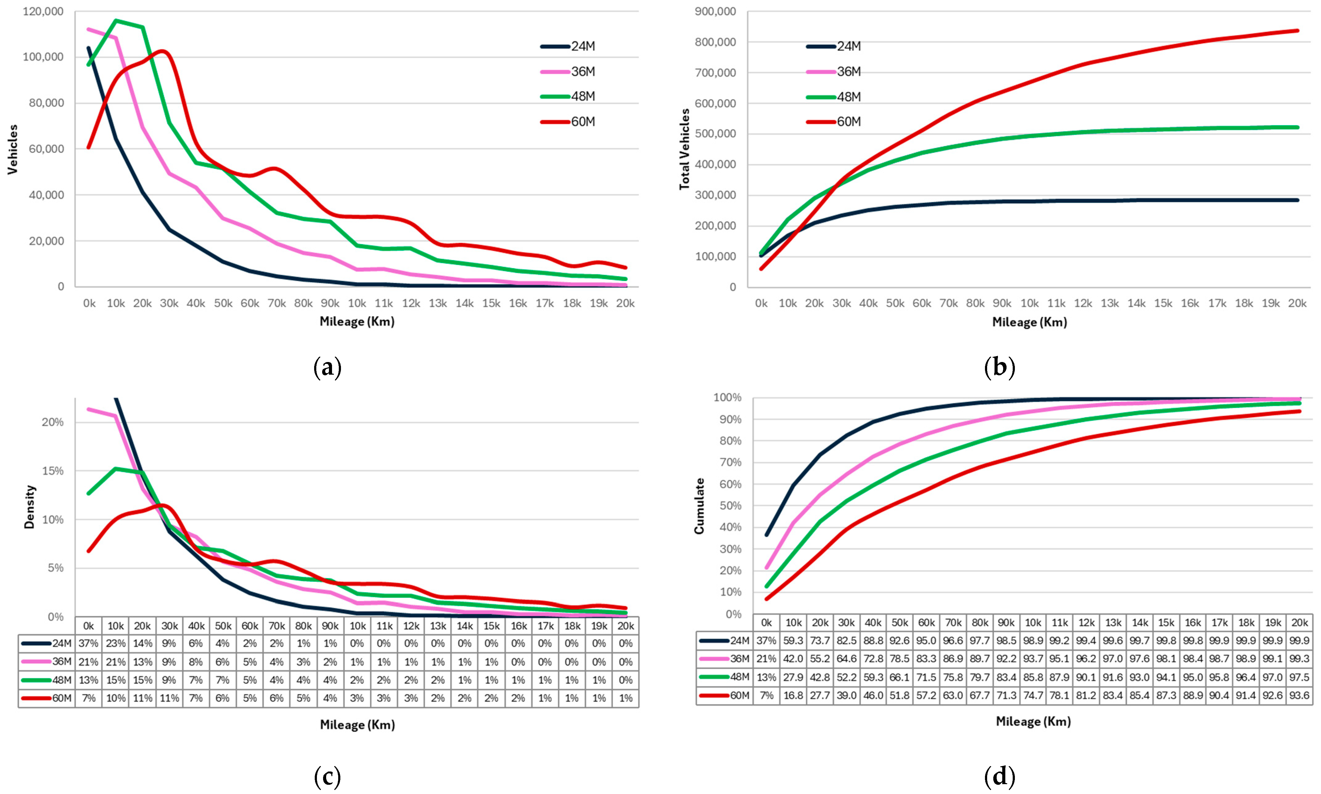
3.6. Fleet Mileage Aging

The same methodology can be similarly applied for different scopes.

Production data, lead time and mileage profile are combined to estimate the vehicle fleet aging at various points in time (i.e., ‘calendar time’). So far, the procedure is used for M38 in the way to estimate the censored data, as this is the moment of updating the failure data, which is used to determine the reliability. Following, the same method is implemented estimating the fleet mileage aging evolution over time. Figure 17 shows this characteristic in the case of 12, 24, 36, 48, 60 months from start of production. Information is provided as PDF and CDF, both in terms of normalized and real data.

As time passes:

• the trend widens and moves towards higher kilometers (e.g., the median moves to 58,000 km in 60 months).
• a peak emerges, becomes more and more pronounced, and it progressively moves to greater kilometers (e.g., the mode to 28,000 km in 60 months).
• an increasingly larger portion leaves the interval under observation (0–210,000 km): from 0.06% after 24 months to 6.43% at 60 months.

3.7. Spare Part Prediction

Merging the fleet mileage aging with the Weibull failure distribution, it is possible to predict failures over time and then, the need of spare parts. Figure 18 shows this information in terms of total failures and of fraction of failures vs. sales.

The failures increase with sales, but not proportionally: this is clear by observing how the gap between the % of failures and sales progressively increases, from 0.08% to 1.06% at 72 months (Figure 18b). This is due to a hazard rate (h) increasing over time (Figure 16d), with the % of failures increasing as fleet mileage aging increases.

3.8. Validation, Uncertainties, and Unpredictability

The proposed estimation is apparently higher, estimating 2970 failures vs. 2675 (+10%) at M38. The method validation is not as simple as it may seem. Hardly, it is enough to wait a to check if predictions agree with reality and that is for several meaningful motivations, attributed, in one manner or another, to issues related to data classification.:

• the systems are subject to frequent redesigns, often occurring ‘behind the scenes’, with the aim of enhancing performance and reliability. Consequently, data inputs could concern products not necessarily identical as supposed. Such ‘in progress’ changes improves when defects occur. Here, e.g., starting from the 30th month, a new design solution is introduced to definitely solve several specific emerged criticalities. Regarding the reliability estimation, given that it is based on data updated to the 38th month, it can be estimated that 25–30% of parts is characterized by the new design, with a growing impact, affecting up to 56% of systems.
• it is important to distinguish when failures result from a process issue, typically transient, or an overall design weakness. In the former case, a specific production batch need to be considered, excluding large part of the population with significant impact on prediction. In the present case, no evidence of being in the presence of a ‘defective batch’ has been identified.
• the way draft data is collected and processed, finally, have to be better considered sometimes. This attention includes, e.g., the way data is classified into discrete intervals, the truncation of distribution tails, and much more. For instance, when the mileages are grouped in intervals (e.g., 10,000 km, as in the present case), it is hard to investigate phenomena under this interval (as early failures, typically occurring in the first 5/8,000 km). And it is not a coincidence that Weibull distribution here determined is not dissimilar from an Exponential function (they coincide in the case of k = 1, instead of =1.2). It identifies a constant hazard rate, representative of occasional failures, not related to early failures or aging.
• a deeper attention to the data classification can be fundamental sometimes, as it could directly impact on accuracy. Among others, geographic-based categories are usually necessary. For example, in the present case, the average annual mileage in (Northern) Europe (34,945) is ~6500 km higher than in North America (27,056). With this difference (~22.8%), the European fleet, just after over four years, is effectively ‘one year older’ (Figure 19). In opposition, the introduction of more categorizations results in less data being available for the analysis, with a consequent loss in accuracy.
• as frequently happens, multiple concomitant failure causes can overlap, each with its own reliability behavior. The use of a single model (e.g., Weibull) can be too approximate. In the case, a subgroup of 122 failed parts is collected and analyzed in laboratory, identifying 6 main failure causes and 50% not trouble found (NTF).
• when the RDA does not identify any issue that seem particularly concerning, the most common car manufacturer’s respond is to close the case, ceasing to commit resources to data acquisition (which may not always be complete and automatic).

Finally, it is not always possible to immediately extend calculations to predict events at distant times, as additional factors often come into play. Over time it increases the number of vehicles:

• experiencing multiple failures (of the same type)
• scrapped from the system due to accidents, permanent breakdowns, or personal choices. This phenomenon commonly starts to be significant around 100/150,000 km, becoming predominant over 250/300,000 km [25].

4. Conclusions and Further Work

This present paper describes a comprehensive reliability data analysis (RDA) performed in the automotive sector. It is focused on the integration of production and failure data to identify appropriate reliability models and make failure predictions. The analysis demands an extensive statistical examination of production and lead times, aimed at determining vehicle sales and deployment. Then, it inserts mileage information to evaluating vehicle fleet aging and detect ‘censored data’, which is used to refine ‘failure data’. By the Kaplan-Meier estimation, data is used for a non-parametric estimation of reliability, before applying the Weibull parametric model for predicting failures over time. Predictions and reality are not too far apart (+10%), and reasons have been discussed, able to justify the difference This research is grounded in real-world data and offers insights from various perspectives, including those of OEMs, Car Manufacturers, and Users.

Further work will aim to expand the scope and depth of the research. A critical focus will be to move beyond the initial assumption of a homogeneous dataset, acknowledging the complex reality of the data. Systems often undergo periodic design modifications. In the context of the present study, e.g., two types of devices within the dataset can be distinguished. In addition, geographical variations, and the presence of data gaps in specific categories of data demand more thorough consideration.

Looking ahead, the most critical areas for future investigation revolve around the refinement and validation of RDA methodologies. On one hand, it will involve testing some of the current assumptions in the way to improve the estimates; on the other, finding adequate data to make predictions under extreme conditions (e.g., long-term predictions, low data consistency, etc.).

References

- Fragassa, C.; Pavlovic, A.; Massimo, S. Using a Total Quality Strategy in a new Practical Approach for Improving the Product Reliability in Automotive Industry. Int. J. Qual. Res. 2014, 8, 297–310. [Google Scholar]
- Sabbagha, O.; Ab Rahman, M.N.; Ismail, W.R.; Hussain, W.M.H.W. Impact of quality management systems and after-sales key performance indicators on automotive industry: A literature review. Proc.-Soc. Behav. Sci. 2016, 224, 68–75. [Google Scholar] [CrossRef]
- Zhu, X.; Jiao, C.; Yuan, T. Optimal decisions on product reliability, sales and promotion under nonrenewable warranties. Reliab. Eng. Syst. Saf. 2019, 192, 106268. [Google Scholar] [CrossRef]
- Lewis, E.E. Introduction to Reliability Engineering, 2nd ed.; McGraw-Hill: New York, NY, USA, 1994. [Google Scholar]
- Dhillon, B.S. Maintainability, Maintenance and Reliability for Engineers; Taylor & Francis Group, LLC: Boca Raton, FL, USA, 2006. [Google Scholar]
- O’Connor, P.; Kleyner, A. Practical Reliability Engineering; John Wiley & Sons: Hoboken, NJ, USA, 2012. [Google Scholar]
- Bertsche, B. Reliability in Automotive and Mechanical Engineering: Determination of Component and System Reliability; Springer Science & Business Media: Berlin/Heidelberg, Germany, 2008. [Google Scholar]
- Guida, M.; Pulcini, G. Automotive reliability inference based on past data and technical knowledge. Reliab. Eng. Syst. Saf. 2002, 76, 129–137. [Google Scholar] [CrossRef]
- Zhang, C.W.; Pan, R.; Goh, T.N. Reliability assessment of high-Quality new products with data scarcity. Int. J. Prod. Res. 2021, 59, 4175–4187. [Google Scholar] [CrossRef]
- Ulbrich, D.; Selech, J.; Kowalczyk, J.; Jóźwiak, J.; Durczak, K.; Gil, L.; Pieniak, D.; Paczkowska, M.; Przystupa, K. Reliability Analysis for Unrepairable Automotive Components. Materials 2021, 14, 7014. [Google Scholar] [CrossRef] [PubMed]
- Ndlovu, B.N.; Ayomoh, M. Reliability Analysis of the Functional Capabilities of an Autonomous Vehicle. Int. J. Math. Eng. Manag. Sci. 2023, 8, 943. [Google Scholar] [CrossRef]
- Zou, T.; Mahadevan, S.; Mourelatos, Z.; Meernik, P. Reliability analysis of automotive body-door subsystem. Reliab. Eng. Syst. Saf. 2002, 78, 315–324. [Google Scholar] [CrossRef]
- Ibrahim, M.; EA, E.A.; Yousof, H.M. A new distribution for modeling lifetime data with different methods of estimation and censored regression modeling. Stat. Optim. Inf. Comput. 2020, 8, 610–630. [Google Scholar] [CrossRef]
- Meeker, W.Q.; Escobar, L.A.; Pascual, F.G. Statistical Methods for Reliability Data; John Wiley & Sons: Hoboken, NJ, USA, 2022. [Google Scholar]
- Lawless, J.F. Statistical Models and Methods for Lifetime Data; John Wiley & Sons, Inc.: New York, NY, USA, 1982. [Google Scholar]
- Deshpande, J.V.; Purohit, S.G. Lifetime Data: Statistical Models and Methods; World Scientific Publishing Company: Singapore, 2015; Volume 16. [Google Scholar]
- Kaplan, E.L.; Meier, P. Nonparametric estimation from incomplete observations. J. Am. Stat. Assoc. 1958, 53, 457–481. [Google Scholar] [CrossRef]
- Weibull, W. A statistical distribution function of wide applicability. Appl. Mech. 1951, 18, 293–297. [Google Scholar]
- Fréchet, M. Sur la loi de probabilité de lécart maximum. Ann. Soc. Pol. Math 1927, 6, 93–116. [Google Scholar]
- Nelson, W. Weibull analysis of reliability data with few or no failures. J. Qual. Technol. 1985, 17, 140–146. [Google Scholar] [CrossRef]
- Guo, J.; Kong, X.; Wu, N.; Xie, L. Weibull parameter estimation and reliability analysis with small samples based on successive approximation method. J. Mech. Sci. Technol. 2023, 37, 5797–5811. [Google Scholar] [CrossRef]
- Elmahdy, E.E. Modelling reliability data with finite weibull or lognormal mixture distributions. Appl. Math. Inf. Sci. 2017, 11, 1081–1089. [Google Scholar] [CrossRef]
- Nelson, W. Applied Life Data Analysis; Addison-Wesley: Boston, MA, USA, 1982. [Google Scholar]
- Genschel, U.; Meeker, W.Q. A Comparison of maximum likelihood and median-rank regression for Weibull estimation. Qual. Eng. 2010, 22, 236–255. [Google Scholar] [CrossRef]
- Brighi, F.; Fragassa, C.; Verratti, L.; Vianello, M. How the Phenomenon of Vehicles Dismantling Influences Reliability Predictions in the Automotive Field. In Proceedings of the 3rd International IMEKO—Youth Symposium on Experimental Solid Mechanics, Porretta Terme, Italy, 12–15 May 2004. [Google Scholar]
Disclaimer/Publisher’s Note: The statements, opinions and data contained in all publications are solely those of the individual author(s) and contributor(s) and not of MDPI and/or the editor(s). MDPI and/or the editor(s) disclaim responsibility for any injury to people or property resulting from any ideas, methods, instructions or products referred to in the content. |
© 2024 by the author. Licensee MDPI, Basel, Switzerland. This article is an open access article distributed under the terms and conditions of the Creative Commons Attribution (CC BY) license (https://creativecommons.org/licenses/by/4.0/).
Share and Cite
Fragassa, C. Analysis of Production and Failure Data in Automotive: From Raw Data to Predictive Modeling and Spare Parts. Mathematics 2024, 12, 510. https://doi.org/10.3390/math12040510
Fragassa C. Analysis of Production and Failure Data in Automotive: From Raw Data to Predictive Modeling and Spare Parts. Mathematics. 2024; 12(4):510. https://doi.org/10.3390/math12040510
Chicago/Turabian StyleFragassa, Cristiano. 2024. "Analysis of Production and Failure Data in Automotive: From Raw Data to Predictive Modeling and Spare Parts" Mathematics 12, no. 4: 510. https://doi.org/10.3390/math12040510
APA StyleFragassa, C. (2024). Analysis of Production and Failure Data in Automotive: From Raw Data to Predictive Modeling and Spare Parts. Mathematics, 12(4), 510. https://doi.org/10.3390/math12040510