
Integrated Profitability Evaluation for a Newsboy-Type Product in Own Brand Manufacturers

Abstract
:1. Introduction
1.1. Problem Statement and Existing Methods
1.2. Research Objective
2. Integrated Profitability
2.1. Formulations of Integrated Profitability and IACI
2.2. Statistical Properties of IACI
2.3. Multiple Samples: Discussion
3. Evaluating Integrated Profitability Using IACI
- (1)
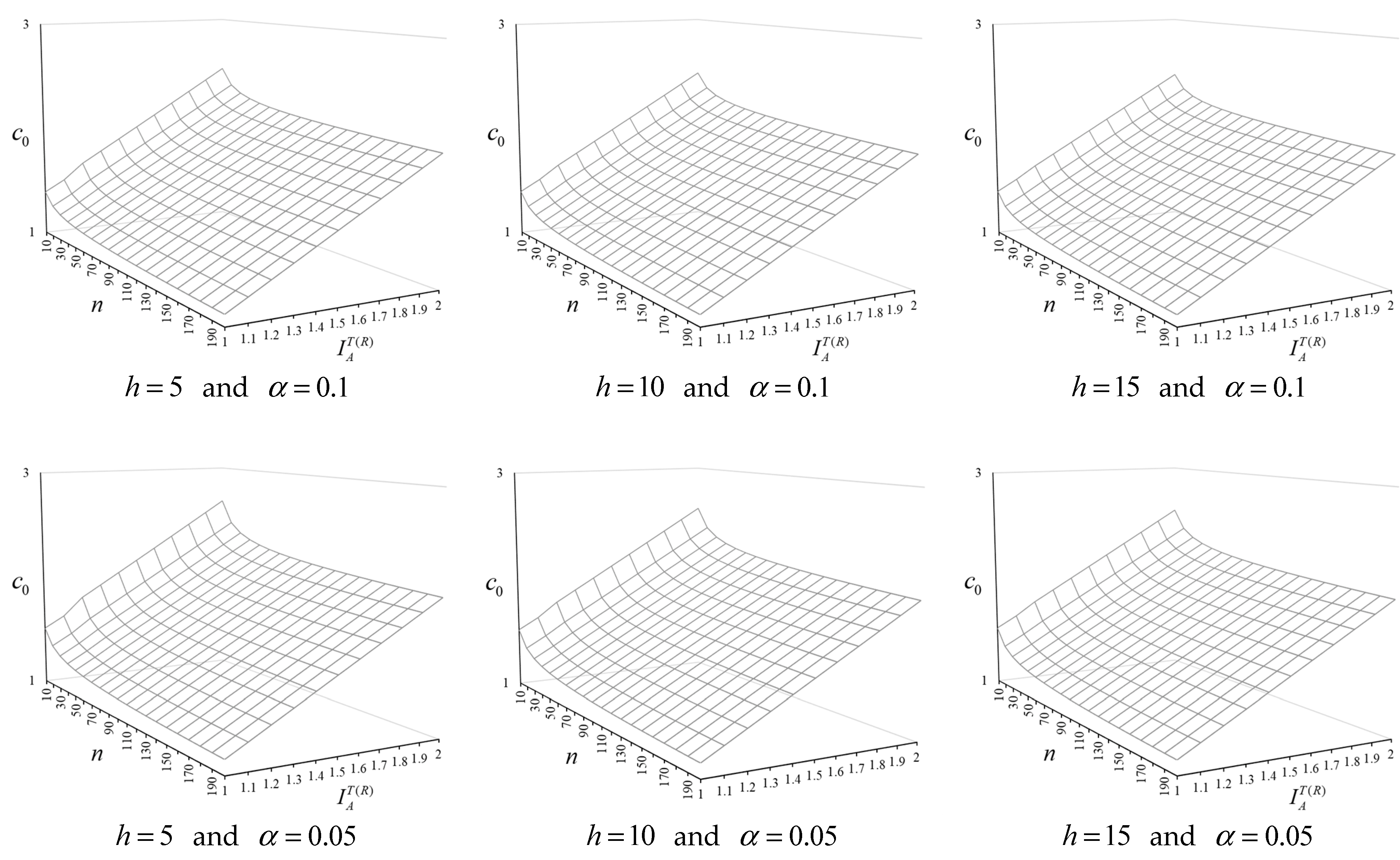
- If the values of , , and were fixed, then the critical value would decrease with an increase in sample size . This means that an increase in sample size would widen the rejection region of the test (i.e., a higher likelihood of falling into the rejection region). Note, however, that increasing the sample size would not necessarily increase the probability of rejecting , due to the fact that estimate could change.
- (2)
- If the values of , , and were fixed, then the critical value would increase with an increase in the stipulated minimum profit . This means that increasing the stipulated minimum profit would reduce the width of the rejection region and thereby reduce the likelihood of rejecting the null hypothesis. This is in line with intuition and statistical inference.
4. Application Example
4.1. OBM Firm
4.2. Numerical Example
- selling price: ;
- manufacturing cost: ;
- net profit per pillow: ;
- total target profit for all channels per cycle: ;
- total target demand for all channels per period: ;
- shortage cost per pillow: ;
- disposal cost per pillow: ;
- excess cost per pillow: ;
- stipulated minimum level for IACI: . The corresponding integrated profitability is .
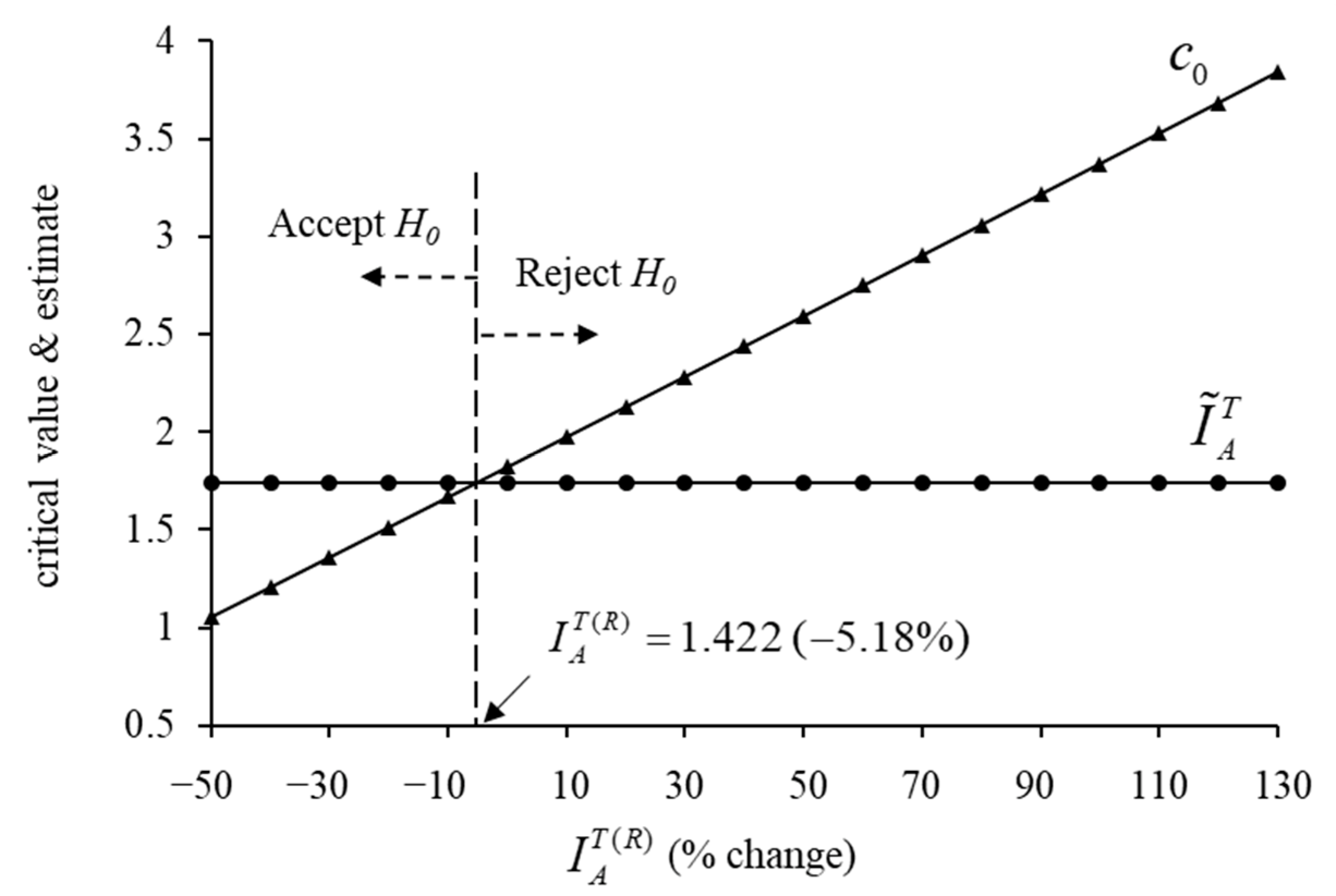
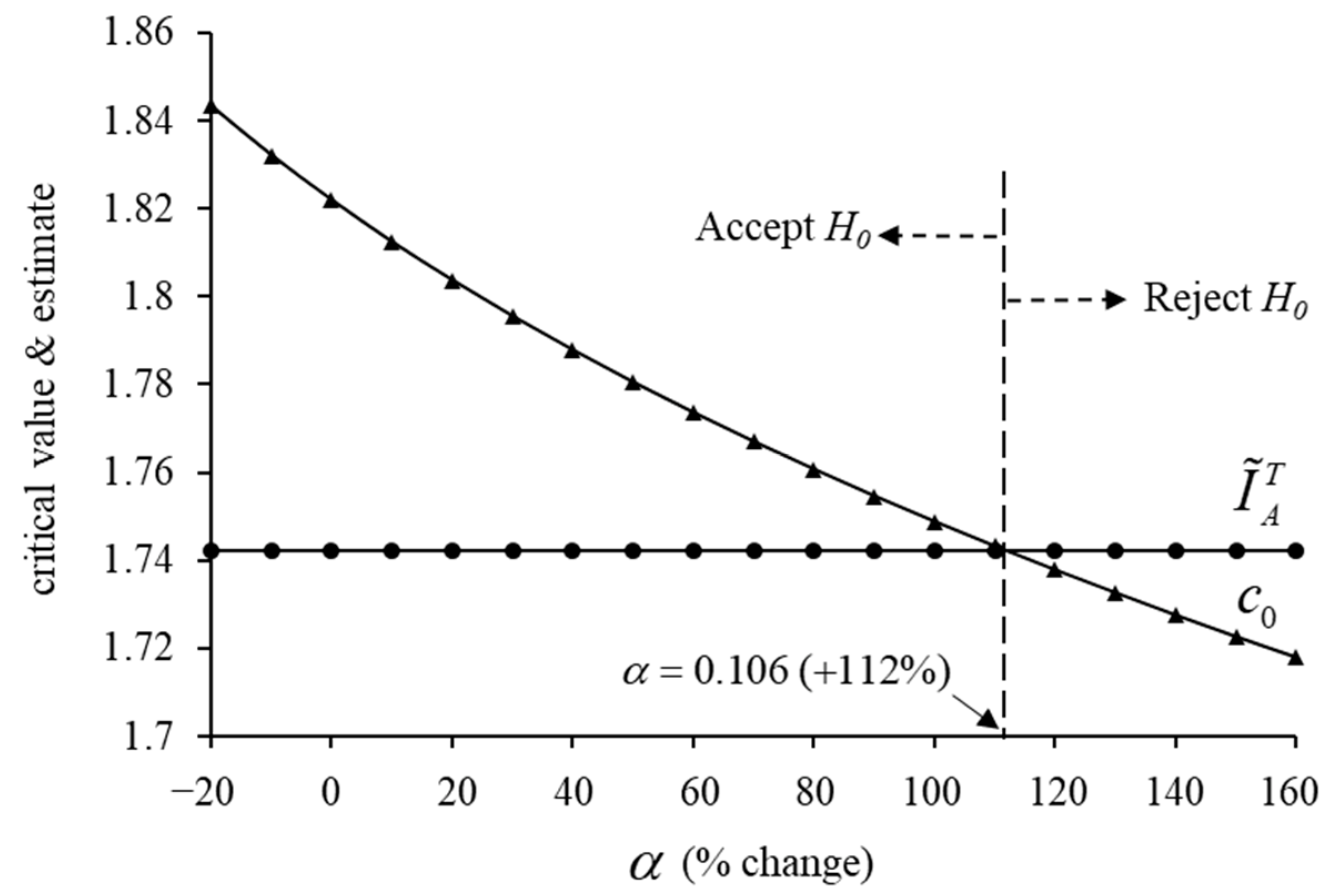
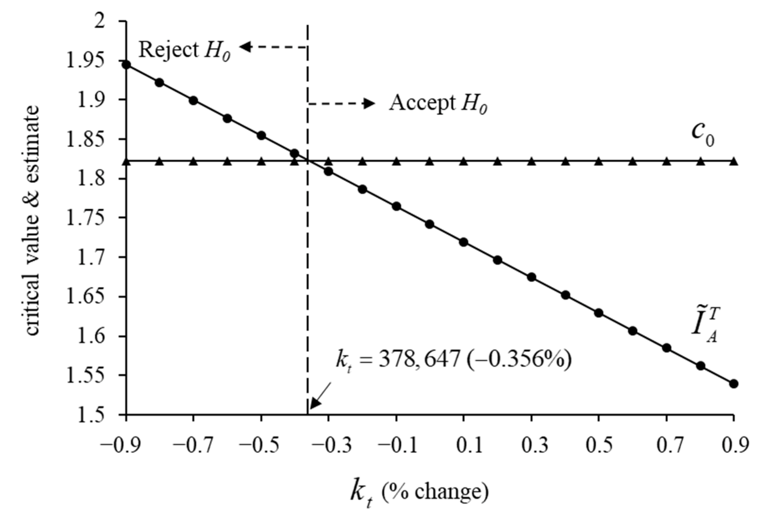
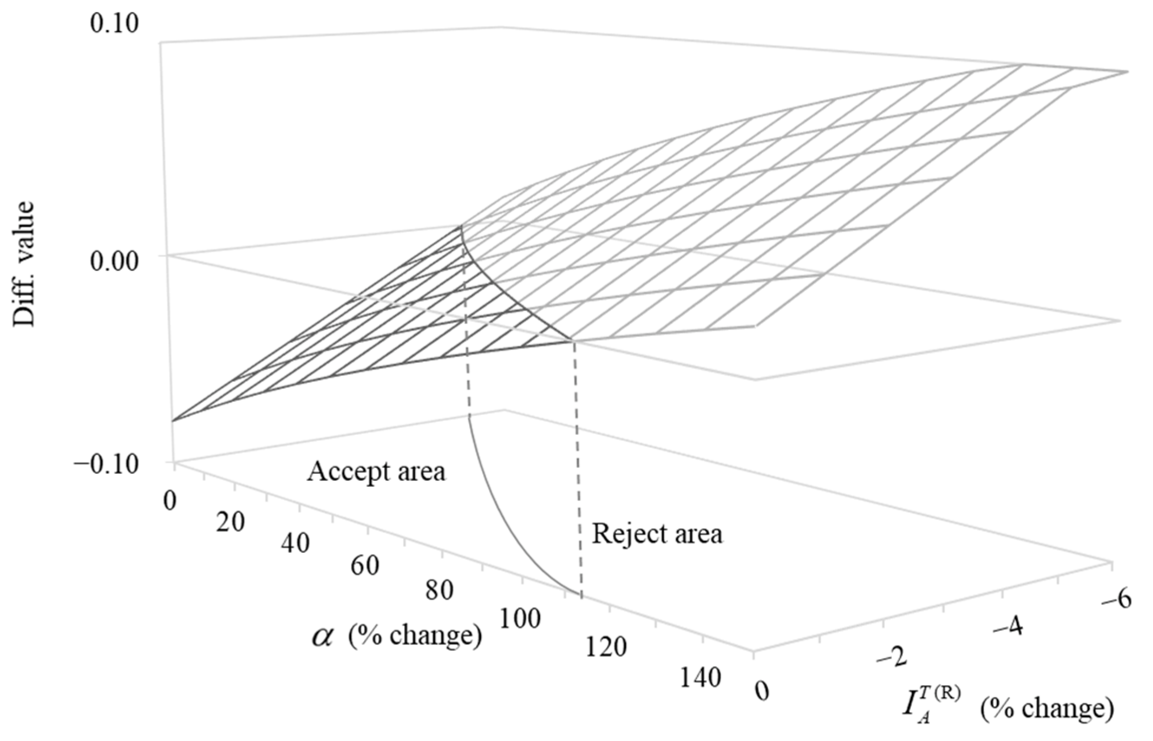
4.3. Sensitivity Analysis
5. Conclusions
- (1)
- In particular environments, the demand data may be collected from multiple samples rather than a single sample. Therefore, we can consider the data collection involving multiple samples, in which the sample size of each group is equal or unequal.
- (2)
- In the current study, the statistical properties of were derived under the assumption that the demand variance was the same in all channels. We recommend further research without this assumption to enhance generalizability.
- (3)
- The use of IACI is limited to situations where demand obeys normal distribution. To enhance the generalizability of the IACI, the sample data can be made to resemble a normal distribution by applying Box–Cox and Yeo–Johnson transformations.
- (4)
- In this study, the demands of each channel are assumed to be mutually exclusive. However, this assumption cannot be fully satisfied in the real-world scenario. To make our method more applicable in the real world, we can develop the IACI index involving the correlation factors among channels.
- (5)
- To gain further managerial insights, it should be possible to establish a feasible loss function for the adjustable parameters (i.e., and ). In cases where the manager desires to change decisions based on integrated profitability, it should be possible to formulate an optimal model aimed at loss minimization involving a combination of and as a decision variable.
Author Contributions
Funding
Data Availability Statement
Conflicts of Interest
References
- Edalatpour, M.A.; Mirzapour Al-e-Hashem, S.M.J.; Fathollahi-Fard, A.M. Combination of pricing and inventory policies for deteriorating products with sustainability considerations. Environ. Dev. Sustain. 2023, 1–41. [Google Scholar] [CrossRef] [PubMed]
- Lee, J.Y. Investing in carbon emissions reduction in the EOQ model. J. Oper. Res. Soc. 2020, 71, 1289–1300. [Google Scholar] [CrossRef]
- Entezaminia, A.; Gharbi, A.; Ouhimmou, M. A joint production and carbon trading policy for unreliable manufacturing systems under cap-and-trade regulation. J. Clean. Prod. 2021, 293, 125973. [Google Scholar] [CrossRef]
- Hasan, M.R.; Roy, T.C.; Daryanto, Y.; Wee, H.M. Optimizing inventory level and technology investment under a carbon tax, cap-and-trade and strict carbon limit regulations. Sustain. Prod. Consum. 2021, 25, 604–621. [Google Scholar] [CrossRef]
- Khanna, A.; Yadav, S. An EOQ model for freshness and stock dependent demand with expiration date under cap-and-trade mechanism. Int. J. Serv. Oper. Inform. 2021, 11, 197–209. [Google Scholar] [CrossRef]
- Qi, Q.; Zhang, R.Q.; Bai, Q. Joint decisions on emission reduction and order quantity by a risk-averse firm under cap-and-trade regulation. Comput. Ind. Eng. 2021, 162, 107783. [Google Scholar] [CrossRef]
- Konstantaras, I.; Skouri, K.; Benkherouf, L. Optimizing inventory decisions for a closed–loop supply chain model under a carbon tax regulatory mechanism. Int. J. Prod. Econ. 2021, 239, 108185. [Google Scholar] [CrossRef]
- Karampour, M.M.; Hajiaghaei-Keshteli, M.; Fathollahi-Fard, A.M.; Tian, G. Metaheuristics for a bi-objective green vendor managed inventory problem in a two-echelon supply chain network. Sci. Iran. 2022, 29, 816–837. [Google Scholar] [CrossRef]
- Zhang, T.; Hao, Y.; Zhu, X. Consignment inventory management in a closed-loop supply chain for deteriorating items under a carbon cap-and-trade regulation. Comput. Ind. Eng. 2022, 171, 108410. [Google Scholar] [CrossRef]
- Hasan, S.M.; Mashud, A.H.M.; Miah, S.; Daryanto, Y.; Lim, M.K.; Tseng, M.L. A green inventory model considering environmental emissions under carbon tax, cap-and-offset, and cap-and-trade regulations. J. Ind. Prod. Eng. 2023, 40, 538–553. [Google Scholar] [CrossRef]
- Maity, S.; Chakraborty, A.; De, S.K.; Pal, M. A study of an EOQ model of green items with the effect of carbon emission under pentagonal intuitionistic dense fuzzy environment. Soft Comput. 2023, 27, 15033–15055. [Google Scholar] [CrossRef]
- San-José, L.A.; Sicilia, J.; Cárdenas-Barrón, L.E.; González-de-la-Rosa, M. A sustainable inventory model for deteriorating items with power demand and full backlogging under a carbon emission tax. Int. J. Prod. Econ. 2024, 268, 109098. [Google Scholar] [CrossRef]
- Bai, Q.; Chen, M. The distributionally robust newsvendor problem with dual sourcing under carbon tax and cap-and-trade regulations. Comput. Ind. Eng. 2016, 98, 260–274. [Google Scholar] [CrossRef]
- Lee, J.; Lee, M.L.; Park, M. A newsboy model with quick response under sustainable carbon cap-n-trade. Sustainability 2018, 10, 1410. [Google Scholar] [CrossRef]
- Qu, S.; Jiang, G.; Ji, Y.; Zhang, G.; Mohamed, N. Newsvendor’s optimal decisions under stochastic demand and cap-and-trade regulation. Environ. Dev. Sustain. 2021, 23, 17764–17787. [Google Scholar] [CrossRef]
- Chen, C.; Zou, B.; Xu, X.; Li, Z. Optimal shipping quantity, product pricing strategies and carbon emissions of online retailers under a new logistics mode. J. Clean. Prod. 2022, 378, 134269. [Google Scholar] [CrossRef]
- Zhao, X.; Xu, J.; Lu, H. Distributionally robust newsvendor model for fresh products under cap-and-offset regulation. Comput. Model. Eng. Sci. 2023, 136, 1813–1833. [Google Scholar] [CrossRef]
- Adhikary, K.; Kar, S. Multi-objective newsboy problem with random-fuzzy demand. Comput. Appl. Math. 2023, 42, 261. [Google Scholar] [CrossRef]
- Gayon, J.P.; Hassoun, M. The newsvendor problem with GHG emissions from waste disposal under cap-and-trade regulation. Int. J. Prod. Res. 2024, 1–21. [Google Scholar] [CrossRef]
- Ma, S.; Jemai, Z.; Sahin, E.; Dallery, Y. The news-vendor problem with drop-shipping and resalable returns. Int. J. Prod. Res. 2017, 55, 6547–6571. [Google Scholar] [CrossRef]
- Ma, S.; Jemai, Z. Inventory rationing for the News-Vendor problem with a drop-shipping option. Appl. Math. Model. 2019, 71, 438–451. [Google Scholar] [CrossRef]
- Xu, L.; Zheng, Y.; Jiang, L. A robust data-driven approach for the newsvendor problem with nonparametric information. Manuf. Serv. Oper. Manag. 2022, 24, 504–523. [Google Scholar] [CrossRef]
- Kou, Y.; Wan, Z. A new data-driven robust optimization approach to multi-item newsboy problems. J. Ind. Manag. Optim. 2022, 19, 197–223. [Google Scholar] [CrossRef]
- Lin, S.; Chen, Y.; Li, Y.; Shen, Z.J.M. Data-driven newsvendor problems regularized by a profit risk constraint. Prod. Oper. Manag. 2022, 31, 1630–1644. [Google Scholar] [CrossRef]
- Neghab, D.P.; Khayyati, S.; Karaesmen, F. An integrated data-driven method using deep learning for a newsvendor problem with unobservable features. Eur. J. Oper. Res. 2022, 302, 482–496. [Google Scholar] [CrossRef]
- Yang, C.H.; Wang, H.T.; Ma, X.; Talluri, S. A data-driven newsvendor problem: A high-dimensional and mixed-frequency method. Int. J. Prod. Econ. 2023, 266, 109042. [Google Scholar] [CrossRef]
- Tian, Y.X.; Zhang, C. An end-to-end deep learning model for solving data-driven newsvendor problem with accessibility to textual review data. Int. J. Prod. Econ. 2023, 265, 109016. [Google Scholar] [CrossRef]
- Chen, Z.Y. Data-driven risk-averse newsvendor problems: Developing the CVaR criteria and support vector machines. Int. J. Prod. Res. 2024, 62, 1221–1238. [Google Scholar] [CrossRef]
- Kevork, I.S. Estimating the optimal order quantity and the maximum expected profit for single-period inventory decisions. Omega-Int. J. Manag. Sci. 2010, 38, 218–227. [Google Scholar] [CrossRef]
- Halkos, G.E.; Kevork, I.S. Unbiased estimation of maximum expected profits in the newsvendor model: A case study analysis. MPRA 2012, e40724. Available online: http://web.archive.org/web/20240127051702/https://mpra.ub.uni-muenchen.de/40724/ (accessed on 24 December 2023).
- Halkos, G.E.; Kevork, I.S. Validity and precision of estimates in the classical newsvendor model with exponential and Rayleigh demand. MPRA 2012, e36460. Available online: http://web.archive.org/web/20240127052059/https://mpra.ub.uni-muenchen.de/36460/ (accessed on 24 December 2023).
- Sundar, D.K.; Ravikumar, K.; Mahajan, S. The distribution free newsboy problem with partial information. Int. J. Oper. Res. 2018, 33, 481–496. [Google Scholar] [CrossRef]
- Su, R.H.; Pearn, W.L. Product selection for newsboy-type products with normal demands and unequal costs. Int. J. Prod. Econ. 2011, 132, 214–222. [Google Scholar] [CrossRef]
- Su, R.H.; Pearn, W.L. Profitability evaluation for newsboy-type product with normally distributed demand. Eur. J. Ind. Eng. 2013, 7, 2–15. [Google Scholar] [CrossRef]
- Su, R.H.; Yang, D.Y.; Pearn, W.L. Assessing profitability of a newsboy-type product with normally distributed demand based on multiple samples. Commun. Stat.-Theory Methods 2013, 42, 3401–3419. [Google Scholar] [CrossRef]
- Su, R.H.; Yang, D.Y.; Pearn, W.L. Estimating and testing achievable capacity index with exponentially distributed demand. Qual. Technol. Quant. Manag. 2015, 12, 221–232. [Google Scholar] [CrossRef]
- Su, R.H.; Wu, C.H.; Yang, D.Y. Conservative profitability evaluation for newsboy-type products using achievable capacity index. Eur. J. Ind. Eng. 2021, 15, 250–272. [Google Scholar] [CrossRef]
- Su, R.H.; Wu, C.H.; Lee, M.H. Conservative profitability evaluation for newsboy-type products with bootstrap methods. Qual. Technol. Quant. Manag. 2022, 19, 74–94. [Google Scholar] [CrossRef]
- Su, R.H.; Yang, D.Y.; Lin, H.J.; Yang, Y.C. Estimating conservative profitability of a newsboy-type product with exponentially distributed demand based on multiple samples. Ann. Oper. Res. 2023, 322, 967–989. [Google Scholar] [CrossRef]
- Ko, Y.Y.; Lin, P.H.; Lin, R.T. A study of service innovation design in cultural and creative industry. Int. Des. Glob. Dev. 2009, 56, 376–385. [Google Scholar] [CrossRef]


| 1.0 | 1.1 | 1.2 | 1.3 | 1.4 | 1.5 | 1.6 | 1.7 | 1.8 | 1.9 | 2.0 | ||
|---|---|---|---|---|---|---|---|---|---|---|---|---|
| 10 | 1.3977 | 1.4982 | 1.6444 | 1.7503 | 1.8566 | 1.9632 | 2.0702 | 2.1774 | 2.2849 | 2.3928 | 2.5009 | |
| 20 | 1.2901 | 1.3913 | 1.5113 | 1.6152 | 1.7192 | 1.8235 | 1.9281 | 2.0328 | 2.1377 | 2.2428 | 2.3481 | |
| 30 | 1.2396 | 1.341 | 1.4533 | 1.5564 | 1.6596 | 1.7630 | 1.8665 | 1.9703 | 2.0742 | 2.1783 | 2.2825 | |
| 40 | 1.2088 | 1.3102 | 1.4190 | 1.5215 | 1.6243 | 1.7272 | 1.8302 | 1.9334 | 2.0367 | 2.1402 | 2.2438 | |
| 50 | 1.1875 | 1.2888 | 1.3956 | 1.4979 | 1.6003 | 1.7029 | 1.8056 | 1.9084 | 2.0113 | 2.1144 | 2.2176 | |
| 60 | 1.1716 | 1.2729 | 1.3784 | 1.4805 | 1.5827 | 1.6850 | 1.7874 | 1.8900 | 1.9926 | 2.0954 | 2.1983 | |
| 70 | 1.1592 | 1.2604 | 1.3651 | 1.4670 | 1.5690 | 1.6711 | 1.7734 | 1.8757 | 1.9782 | 2.0807 | 2.1834 | |
| 80 | 1.1491 | 1.2503 | 1.3543 | 1.4561 | 1.5580 | 1.6599 | 1.7620 | 1.8642 | 1.9665 | 2.0689 | 2.1714 | |
| 90 | 1.1408 | 1.2419 | 1.3454 | 1.4471 | 1.5488 | 1.6507 | 1.7527 | 1.8547 | 1.9569 | 2.0591 | 2.1615 | |
| 100 | 1.1337 | 1.2348 | 1.3379 | 1.4395 | 1.5411 | 1.6429 | 1.7448 | 1.8467 | 1.9488 | 2.0509 | 2.1531 | |
| 110 | 1.1275 | 1.2286 | 1.3315 | 1.4329 | 1.5345 | 1.6362 | 1.7380 | 1.8398 | 1.9418 | 2.0438 | 2.1459 | |
| 120 | 1.1222 | 1.2232 | 1.3258 | 1.4272 | 1.5288 | 1.6304 | 1.7321 | 1.8338 | 1.9357 | 2.0376 | 2.1396 | |
| 130 | 1.1174 | 1.2185 | 1.3209 | 1.4222 | 1.5237 | 1.6252 | 1.7268 | 1.8285 | 1.9303 | 2.0322 | 2.1341 | |
| 140 | 1.1132 | 1.2142 | 1.3164 | 1.4177 | 1.5191 | 1.6206 | 1.7222 | 1.8238 | 1.9255 | 2.0273 | 2.1292 | |
| 150 | 1.1094 | 1.2104 | 1.3125 | 1.4137 | 1.5151 | 1.6165 | 1.7180 | 1.8196 | 1.9212 | 2.0230 | 2.1248 | |
| 160 | 1.1060 | 1.2069 | 1.3089 | 1.4101 | 1.5114 | 1.6128 | 1.7142 | 1.8158 | 1.9174 | 2.0190 | 2.1208 | |
| 170 | 1.1028 | 1.2037 | 1.3056 | 1.4068 | 1.5081 | 1.6094 | 1.7108 | 1.8123 | 1.9138 | 2.0154 | 2.1171 | |
| 180 | 1.1000 | 1.2009 | 1.3026 | 1.4038 | 1.5050 | 1.6063 | 1.7077 | 1.8091 | 1.9106 | 2.0122 | 2.1138 | |
| 190 | 1.0973 | 1.1982 | 1.2999 | 1.4010 | 1.5022 | 1.6034 | 1.7048 | 1.8062 | 1.9076 | 2.0092 | 2.1107 | |
| 200 | 1.0949 | 1.1957 | 1.2973 | 1.3984 | 1.4996 | 1.6008 | 1.7021 | 1.8035 | 1.9049 | 2.0064 | 2.1079 | |
| 1.0 | 1.1 | 1.2 | 1.3 | 1.4 | 1.5 | 1.6 | 1.7 | 1.8 | 1.9 | 2.0 | ||
|---|---|---|---|---|---|---|---|---|---|---|---|---|
| 10 | 1.4016 | 1.5018 | 1.6251 | 1.7281 | 1.8314 | 1.9349 | 2.0385 | 2.1423 | 2.2463 | 2.3505 | 2.4548 | |
| 20 | 1.2883 | 1.3890 | 1.4991 | 1.6011 | 1.7032 | 1.8055 | 1.9078 | 2.0103 | 2.1129 | 2.2157 | 2.3185 | |
| 30 | 1.2368 | 1.3375 | 1.4438 | 1.5454 | 1.6470 | 1.7488 | 1.8507 | 1.9527 | 2.0547 | 2.1569 | 2.2592 | |
| 40 | 1.2058 | 1.3065 | 1.4109 | 1.5123 | 1.6137 | 1.7152 | 1.8168 | 1.9185 | 2.0202 | 2.1221 | 2.2240 | |
| 50 | 1.1844 | 1.2851 | 1.3885 | 1.4897 | 1.5910 | 1.6923 | 1.7937 | 1.8952 | 1.9968 | 2.0984 | 2.2001 | |
| 60 | 1.1686 | 1.2692 | 1.3720 | 1.4731 | 1.5742 | 1.6754 | 1.7767 | 1.8781 | 1.9795 | 2.0810 | 2.1825 | |
| 70 | 1.1562 | 1.2569 | 1.3592 | 1.4602 | 1.5612 | 1.6624 | 1.7635 | 1.8648 | 1.9661 | 2.0675 | 2.1689 | |
| 80 | 1.1462 | 1.2468 | 1.3489 | 1.4498 | 1.5508 | 1.6518 | 1.7529 | 1.8541 | 1.9553 | 2.0566 | 2.1579 | |
| 90 | 1.1380 | 1.2385 | 1.3403 | 1.4412 | 1.5421 | 1.6431 | 1.7441 | 1.8452 | 1.9464 | 2.0476 | 2.1488 | |
| 100 | 1.1309 | 1.2315 | 1.3331 | 1.4339 | 1.5348 | 1.6357 | 1.7367 | 1.8377 | 1.9388 | 2.0399 | 2.1411 | |
| 110 | 1.1249 | 1.2254 | 1.3269 | 1.4277 | 1.5285 | 1.6294 | 1.7303 | 1.8313 | 1.9323 | 2.0334 | 2.1345 | |
| 120 | 1.1196 | 1.2201 | 1.3215 | 1.4222 | 1.5230 | 1.6238 | 1.7247 | 1.8257 | 1.9267 | 2.0277 | 2.1288 | |
| 130 | 1.1149 | 1.2155 | 1.3167 | 1.4174 | 1.5182 | 1.6190 | 1.7198 | 1.8207 | 1.9217 | 2.0227 | 2.1237 | |
| 140 | 1.1108 | 1.2113 | 1.3124 | 1.4131 | 1.5138 | 1.6146 | 1.7154 | 1.8163 | 1.9172 | 2.0182 | 2.1192 | |
| 150 | 1.1071 | 1.2075 | 1.3086 | 1.4093 | 1.5100 | 1.6107 | 1.7115 | 1.8123 | 1.9132 | 2.0141 | 2.1151 | |
| 160 | 1.1037 | 1.2041 | 1.3052 | 1.4058 | 1.5065 | 1.6072 | 1.7080 | 1.8088 | 1.9096 | 2.0105 | 2.1114 | |
| 170 | 1.1006 | 1.2011 | 1.3020 | 1.4026 | 1.5033 | 1.6040 | 1.7047 | 1.8055 | 1.9063 | 2.0072 | 2.1081 | |
| 180 | 1.0978 | 1.1982 | 1.2991 | 1.3997 | 1.5004 | 1.6010 | 1.7018 | 1.8025 | 1.9033 | 2.0042 | 2.1050 | |
| 190 | 1.0952 | 1.1956 | 1.2965 | 1.3971 | 1.4977 | 1.5983 | 1.6990 | 1.7998 | 1.9006 | 2.0014 | 2.1022 | |
| 200 | 1.0928 | 1.1932 | 1.2940 | 1.3946 | 1.4952 | 1.5958 | 1.6965 | 1.7972 | 1.8980 | 1.9988 | 2.0996 | |
| 1.0 | 1.1 | 1.2 | 1.3 | 1.4 | 1.5 | 1.6 | 1.7 | 1.8 | 1.9 | 2.0 | ||
|---|---|---|---|---|---|---|---|---|---|---|---|---|
| 10 | 1.4028 | 1.5030 | 1.6185 | 1.7206 | 1.8228 | 1.9251 | 2.0276 | 2.1302 | 2.2329 | 2.3358 | 2.4388 | |
| 20 | 1.2878 | 1.3882 | 1.4950 | 1.5963 | 1.6977 | 1.7993 | 1.9009 | 2.0026 | 2.1044 | 2.2062 | 2.3082 | |
| 30 | 1.2359 | 1.3364 | 1.4406 | 1.5416 | 1.6427 | 1.7439 | 1.8452 | 1.9466 | 2.0480 | 2.1495 | 2.2510 | |
| 40 | 1.2047 | 1.3052 | 1.4082 | 1.5091 | 1.6100 | 1.7111 | 1.8122 | 1.9133 | 2.0145 | 2.1158 | 2.2171 | |
| 50 | 1.1834 | 1.2838 | 1.3861 | 1.4869 | 1.5878 | 1.6887 | 1.7896 | 1.8907 | 1.9917 | 2.0928 | 2.1940 | |
| 60 | 1.1675 | 1.2680 | 1.3699 | 1.4706 | 1.5713 | 1.6722 | 1.7730 | 1.8740 | 1.9749 | 2.0759 | 2.1770 | |
| 70 | 1.1552 | 1.2556 | 1.3572 | 1.4579 | 1.5586 | 1.6593 | 1.7601 | 1.8610 | 1.9619 | 2.0628 | 2.1638 | |
| 80 | 1.1453 | 1.2457 | 1.3470 | 1.4477 | 1.5483 | 1.6490 | 1.7498 | 1.8506 | 1.9514 | 2.0523 | 2.1532 | |
| 90 | 1.1370 | 1.2374 | 1.3386 | 1.4392 | 1.5398 | 1.6405 | 1.7412 | 1.8419 | 1.9427 | 2.0435 | 2.1444 | |
| 100 | 1.1300 | 1.2304 | 1.3315 | 1.4320 | 1.5326 | 1.6332 | 1.7339 | 1.8346 | 1.9353 | 2.0361 | 2.1369 | |
| 110 | 1.1240 | 1.2244 | 1.3253 | 1.4259 | 1.5264 | 1.6270 | 1.7276 | 1.8283 | 1.9290 | 2.0298 | 2.1305 | |
| 120 | 1.1187 | 1.2191 | 1.3200 | 1.4205 | 1.5210 | 1.6216 | 1.7222 | 1.8228 | 1.9235 | 2.0242 | 2.1250 | |
| 130 | 1.1141 | 1.2145 | 1.3153 | 1.4158 | 1.5163 | 1.6168 | 1.7174 | 1.8180 | 1.9186 | 2.0193 | 2.1200 | |
| 140 | 1.1100 | 1.2103 | 1.3111 | 1.4115 | 1.5120 | 1.6126 | 1.7131 | 1.8137 | 1.9143 | 2.0150 | 2.1157 | |
| 150 | 1.1063 | 1.2066 | 1.3073 | 1.4077 | 1.5082 | 1.6087 | 1.7093 | 1.8098 | 1.9104 | 2.0111 | 2.1117 | |
| 160 | 1.1029 | 1.2032 | 1.3039 | 1.4043 | 1.5048 | 1.6053 | 1.7058 | 1.8063 | 1.9069 | 2.0075 | 2.1082 | |
| 170 | 1.0998 | 1.2001 | 1.3008 | 1.4012 | 1.5016 | 1.6021 | 1.7026 | 1.8032 | 1.9037 | 2.0043 | 2.1049 | |
| 180 | 1.0970 | 1.1973 | 1.2979 | 1.3983 | 1.4988 | 1.5992 | 1.6997 | 1.8002 | 1.9008 | 2.0014 | 2.1020 | |
| 190 | 1.0944 | 1.1947 | 1.2953 | 1.3957 | 1.4961 | 1.5966 | 1.6971 | 1.7976 | 1.8981 | 1.9986 | 2.0992 | |
| 200 | 1.0921 | 1.1924 | 1.2929 | 1.3933 | 1.4937 | 1.5941 | 1.6946 | 1.7951 | 1.8956 | 1.9961 | 2.0967 | |
| 1.0 | 1.1 | 1.2 | 1.3 | 1.4 | 1.5 | 1.6 | 1.7 | 1.8 | 1.9 | 2.0 | ||
|---|---|---|---|---|---|---|---|---|---|---|---|---|
| 10 | 1.5177 | 1.6190 | 1.7856 | 1.8942 | 2.0033 | 2.1127 | 2.2226 | 2.3329 | 2.4435 | 2.5545 | 2.6659 | |
| 20 | 1.3762 | 1.4781 | 1.6062 | 1.7116 | 1.8173 | 1.9233 | 2.0295 | 2.1360 | 2.2428 | 2.3498 | 2.4570 | |
| 30 | 1.3103 | 1.4123 | 1.5293 | 1.6335 | 1.7379 | 1.8426 | 1.9475 | 2.0526 | 2.1579 | 2.2634 | 2.3690 | |
| 40 | 1.2701 | 1.3721 | 1.4841 | 1.5876 | 1.6913 | 1.7953 | 1.8994 | 2.0037 | 2.1082 | 2.2128 | 2.3177 | |
| 50 | 1.2424 | 1.3442 | 1.4535 | 1.5565 | 1.6598 | 1.7633 | 1.8669 | 1.9707 | 2.0747 | 2.1788 | 2.2830 | |
| 60 | 1.2217 | 1.3235 | 1.4309 | 1.5337 | 1.6367 | 1.7398 | 1.8431 | 1.9465 | 2.0501 | 2.1538 | 2.2576 | |
| 70 | 1.2056 | 1.3073 | 1.4135 | 1.5161 | 1.6188 | 1.7216 | 1.8246 | 1.9278 | 2.0311 | 2.1345 | 2.2380 | |
| 80 | 1.1925 | 1.2941 | 1.3995 | 1.5019 | 1.6044 | 1.7070 | 1.8098 | 1.9128 | 2.0158 | 2.1190 | 2.2223 | |
| 90 | 1.1816 | 1.2832 | 1.3879 | 1.4901 | 1.5925 | 1.6950 | 1.7976 | 1.9004 | 2.0032 | 2.1062 | 2.2093 | |
| 100 | 1.1724 | 1.2739 | 1.3781 | 1.4802 | 1.5825 | 1.6848 | 1.7873 | 1.8899 | 1.9926 | 2.0954 | 2.1983 | |
| 110 | 1.1645 | 1.2659 | 1.3697 | 1.4717 | 1.5739 | 1.6761 | 1.7784 | 1.8809 | 1.9835 | 2.0861 | 2.1889 | |
| 120 | 1.1575 | 1.2590 | 1.3624 | 1.4643 | 1.5663 | 1.6685 | 1.7707 | 1.8731 | 1.9755 | 2.0781 | 2.1807 | |
| 130 | 1.1514 | 1.2528 | 1.3560 | 1.4578 | 1.5597 | 1.6618 | 1.7639 | 1.8662 | 1.9685 | 2.0710 | 2.1735 | |
| 140 | 1.1459 | 1.2473 | 1.3502 | 1.4520 | 1.5538 | 1.6558 | 1.7579 | 1.8600 | 1.9623 | 2.0646 | 2.1671 | |
| 150 | 1.1410 | 1.2423 | 1.3451 | 1.4468 | 1.5486 | 1.6505 | 1.7524 | 1.8545 | 1.9567 | 2.0590 | 2.1613 | |
| 160 | 1.1366 | 1.2378 | 1.3404 | 1.4421 | 1.5438 | 1.6456 | 1.7475 | 1.8495 | 1.9516 | 2.0538 | 2.1561 | |
| 170 | 1.1325 | 1.2337 | 1.3362 | 1.4378 | 1.5394 | 1.6412 | 1.7431 | 1.8450 | 1.9471 | 2.0492 | 2.1514 | |
| 180 | 1.1288 | 1.2300 | 1.3323 | 1.4339 | 1.5355 | 1.6372 | 1.7390 | 1.8409 | 1.9429 | 2.0449 | 2.1470 | |
| 190 | 1.1254 | 1.2265 | 1.3288 | 1.4302 | 1.5318 | 1.6335 | 1.7352 | 1.8371 | 1.9390 | 2.0410 | 2.1431 | |
| 200 | 1.1222 | 1.2233 | 1.3255 | 1.4269 | 1.5284 | 1.6301 | 1.7318 | 1.8336 | 1.9354 | 2.0374 | 2.1394 | |
| 1.0 | 1.1 | 1.2 | 1.3 | 1.4 | 1.5 | 1.6 | 1.7 | 1.8 | 1.9 | 2.0 | ||
|---|---|---|---|---|---|---|---|---|---|---|---|---|
| 10 | 1.5190 | 1.6197 | 1.7531 | 1.8575 | 1.9622 | 2.0671 | 2.1722 | 2.2776 | 2.3833 | 2.4891 | 2.5951 | |
| 20 | 1.3720 | 1.4730 | 1.5872 | 1.6900 | 1.7929 | 1.8961 | 1.9993 | 2.1027 | 2.2063 | 2.3101 | 2.4139 | |
| 30 | 1.3053 | 1.4064 | 1.5150 | 1.6172 | 1.7195 | 1.8219 | 1.9244 | 2.0271 | 2.1299 | 2.2329 | 2.3359 | |
| 40 | 1.2651 | 1.3661 | 1.4722 | 1.5741 | 1.6760 | 1.7781 | 1.8802 | 1.9825 | 2.0849 | 2.1874 | 2.2899 | |
| 50 | 1.2375 | 1.3385 | 1.4432 | 1.5448 | 1.6465 | 1.7483 | 1.8502 | 1.9522 | 2.0543 | 2.1565 | 2.2588 | |
| 60 | 1.2171 | 1.3180 | 1.4218 | 1.5232 | 1.6248 | 1.7264 | 1.8281 | 1.9299 | 2.0318 | 2.1338 | 2.2359 | |
| 70 | 1.2011 | 1.3020 | 1.4052 | 1.5065 | 1.6079 | 1.7094 | 1.8110 | 1.9126 | 2.0144 | 2.1162 | 2.2181 | |
| 80 | 1.1882 | 1.2891 | 1.3918 | 1.4930 | 1.5944 | 1.6957 | 1.7972 | 1.8987 | 2.0004 | 2.1021 | 2.2038 | |
| 90 | 1.1776 | 1.2783 | 1.3808 | 1.4819 | 1.5831 | 1.6844 | 1.7858 | 1.8873 | 1.9888 | 2.0904 | 2.1920 | |
| 100 | 1.1685 | 1.2693 | 1.3714 | 1.4725 | 1.5737 | 1.6749 | 1.7762 | 1.8776 | 1.9790 | 2.0805 | 2.1821 | |
| 110 | 1.1607 | 1.2614 | 1.3634 | 1.4644 | 1.5655 | 1.6667 | 1.7679 | 1.8692 | 1.9706 | 2.0720 | 2.1735 | |
| 120 | 1.1539 | 1.2546 | 1.3564 | 1.4574 | 1.5584 | 1.6595 | 1.7607 | 1.8619 | 1.9632 | 2.0646 | 2.1660 | |
| 130 | 1.1479 | 1.2486 | 1.3502 | 1.4512 | 1.5522 | 1.6532 | 1.7543 | 1.8555 | 1.9568 | 2.0581 | 2.1595 | |
| 140 | 1.1425 | 1.2432 | 1.3447 | 1.4456 | 1.5466 | 1.6476 | 1.7487 | 1.8498 | 1.9510 | 2.0523 | 2.1536 | |
| 150 | 1.1377 | 1.2384 | 1.3398 | 1.4407 | 1.5416 | 1.6426 | 1.7436 | 1.8447 | 1.9459 | 2.0471 | 2.1483 | |
| 160 | 1.1333 | 1.2340 | 1.3353 | 1.4362 | 1.5371 | 1.6380 | 1.7390 | 1.8401 | 1.9412 | 2.0424 | 2.1436 | |
| 170 | 1.1294 | 1.2300 | 1.3313 | 1.4321 | 1.5329 | 1.6339 | 1.7348 | 1.8359 | 1.9370 | 2.0381 | 2.1393 | |
| 180 | 1.1257 | 1.2263 | 1.3275 | 1.4283 | 1.5292 | 1.6301 | 1.7310 | 1.8320 | 1.9331 | 2.0342 | 2.1353 | |
| 190 | 1.1224 | 1.2230 | 1.3241 | 1.4249 | 1.5257 | 1.6266 | 1.7275 | 1.8285 | 1.9295 | 2.0306 | 2.1317 | |
| 200 | 1.1193 | 1.2199 | 1.3210 | 1.4217 | 1.5225 | 1.6234 | 1.7243 | 1.8252 | 1.9262 | 2.0272 | 2.1283 | |
| 1.0 | 1.1 | 1.2 | 1.3 | 1.4 | 1.5 | 1.6 | 1.7 | 1.8 | 1.9 | 2.0 | ||
|---|---|---|---|---|---|---|---|---|---|---|---|---|
| 10 | 1.5194 | 1.6199 | 1.7422 | 1.8451 | 1.9483 | 2.0516 | 2.1551 | 2.2588 | 2.3626 | 2.4666 | 2.5707 | |
| 20 | 1.3706 | 1.4713 | 1.5808 | 1.6827 | 1.7847 | 1.8868 | 1.9890 | 2.0913 | 2.1937 | 2.2963 | 2.3989 | |
| 30 | 1.3037 | 1.4044 | 1.5101 | 1.6116 | 1.7132 | 1.8148 | 1.9165 | 2.0184 | 2.1203 | 2.2223 | 2.3244 | |
| 40 | 1.2635 | 1.3641 | 1.4682 | 1.5695 | 1.6708 | 1.7721 | 1.8736 | 1.9752 | 2.0768 | 2.1785 | 2.2803 | |
| 50 | 1.2359 | 1.3365 | 1.4397 | 1.5408 | 1.6419 | 1.7431 | 1.8444 | 1.9458 | 2.0472 | 2.1487 | 2.2503 | |
| 60 | 1.2155 | 1.3161 | 1.4187 | 1.5196 | 1.6207 | 1.7218 | 1.8229 | 1.9242 | 2.0255 | 2.1268 | 2.2282 | |
| 70 | 1.1996 | 1.3002 | 1.4023 | 1.5032 | 1.6042 | 1.7052 | 1.8063 | 1.9074 | 2.0086 | 2.1098 | 2.2111 | |
| 80 | 1.1868 | 1.2874 | 1.3892 | 1.4900 | 1.5909 | 1.6919 | 1.7929 | 1.8939 | 1.9950 | 2.0962 | 2.1974 | |
| 90 | 1.1762 | 1.2767 | 1.3783 | 1.4791 | 1.5799 | 1.6808 | 1.7817 | 1.8827 | 1.9838 | 2.0849 | 2.1860 | |
| 100 | 1.1672 | 1.2677 | 1.3691 | 1.4699 | 1.5706 | 1.6715 | 1.7724 | 1.8733 | 1.9743 | 2.0753 | 2.1764 | |
| 110 | 1.1594 | 1.2599 | 1.3612 | 1.4619 | 1.5627 | 1.6635 | 1.7643 | 1.8652 | 1.9661 | 2.0671 | 2.1681 | |
| 120 | 1.1527 | 1.2531 | 1.3543 | 1.4550 | 1.5557 | 1.6565 | 1.7573 | 1.8581 | 1.9590 | 2.0599 | 2.1609 | |
| 130 | 1.1467 | 1.2471 | 1.3483 | 1.4489 | 1.5496 | 1.6503 | 1.7511 | 1.8519 | 1.9527 | 2.0536 | 2.1545 | |
| 140 | 1.1414 | 1.2418 | 1.3428 | 1.4434 | 1.5441 | 1.6448 | 1.7455 | 1.8463 | 1.9471 | 2.0480 | 2.1489 | |
| 150 | 1.1366 | 1.2370 | 1.3380 | 1.4386 | 1.5392 | 1.6399 | 1.7406 | 1.8413 | 1.9421 | 2.0429 | 2.1438 | |
| 160 | 1.1322 | 1.2327 | 1.3336 | 1.4341 | 1.5348 | 1.6354 | 1.7361 | 1.8368 | 1.9376 | 2.0384 | 2.1392 | |
| 170 | 1.1283 | 1.2287 | 1.3296 | 1.4301 | 1.5307 | 1.6313 | 1.7320 | 1.8327 | 1.9334 | 2.0342 | 2.1350 | |
| 180 | 1.1247 | 1.2251 | 1.3259 | 1.4264 | 1.5270 | 1.6276 | 1.7283 | 1.8289 | 1.9297 | 2.0304 | 2.1312 | |
| 190 | 1.1214 | 1.2218 | 1.3225 | 1.4231 | 1.5236 | 1.6242 | 1.7248 | 1.8255 | 1.9262 | 2.0269 | 2.1277 | |
| 200 | 1.1183 | 1.2187 | 1.3194 | 1.4199 | 1.5205 | 1.6210 | 1.7217 | 1.8223 | 1.9230 | 2.0237 | 2.1244 | |
| 1.0 | 1.1 | 1.2 | 1.3 | 1.4 | 1.5 | 1.6 | 1.7 | 1.8 | 1.9 | 2.0 | ||
|---|---|---|---|---|---|---|---|---|---|---|---|---|
| 10 | 1.7474 | 1.8504 | 2.0683 | 2.1828 | 2.2979 | 2.4137 | 2.5300 | 2.6469 | 2.7643 | 2.8822 | 3.0006 | |
| 20 | 1.5407 | 1.6442 | 1.7913 | 1.9000 | 2.0091 | 2.1186 | 2.2284 | 2.3387 | 2.4493 | 2.5603 | 2.6715 | |
| 30 | 1.4450 | 1.5483 | 1.6762 | 1.7828 | 1.8897 | 1.9970 | 2.1046 | 2.2124 | 2.3206 | 2.4290 | 2.5377 | |
| 40 | 1.3868 | 1.4900 | 1.6093 | 1.7148 | 1.8205 | 1.9266 | 2.0329 | 2.1395 | 2.2464 | 2.3534 | 2.4607 | |
| 50 | 1.3467 | 1.4497 | 1.5643 | 1.6691 | 1.7741 | 1.8794 | 1.9849 | 2.0907 | 2.1966 | 2.3028 | 2.4092 | |
| 60 | 1.3169 | 1.4197 | 1.5314 | 1.6357 | 1.7402 | 1.8449 | 1.9499 | 2.0550 | 2.1604 | 2.2660 | 2.3717 | |
| 70 | 1.2936 | 1.3963 | 1.5060 | 1.6099 | 1.7140 | 1.8183 | 1.9229 | 2.0276 | 2.1325 | 2.2376 | 2.3429 | |
| 80 | 1.2748 | 1.3773 | 1.4856 | 1.5892 | 1.6930 | 1.7970 | 1.9012 | 2.0056 | 2.1102 | 2.2149 | 2.3198 | |
| 90 | 1.2592 | 1.3616 | 1.4688 | 1.5722 | 1.6758 | 1.7795 | 1.8834 | 1.9875 | 2.0917 | 2.1962 | 2.3007 | |
| 100 | 1.2459 | 1.3482 | 1.4547 | 1.5578 | 1.6612 | 1.7647 | 1.8684 | 1.9722 | 2.0763 | 2.1804 | 2.2847 | |
| 110 | 1.2345 | 1.3367 | 1.4425 | 1.5455 | 1.6487 | 1.7520 | 1.8555 | 1.9592 | 2.0630 | 2.1669 | 2.2710 | |
| 120 | 1.2245 | 1.3267 | 1.4320 | 1.5348 | 1.6378 | 1.7410 | 1.8443 | 1.9478 | 2.0514 | 2.1552 | 2.2591 | |
| 130 | 1.2157 | 1.3178 | 1.4227 | 1.5254 | 1.6283 | 1.7313 | 1.8345 | 1.9378 | 2.0413 | 2.1449 | 2.2486 | |
| 140 | 1.2079 | 1.3099 | 1.4144 | 1.5170 | 1.6198 | 1.7227 | 1.8257 | 1.9289 | 2.0322 | 2.1357 | 2.2393 | |
| 150 | 1.2008 | 1.3028 | 1.4070 | 1.5095 | 1.6121 | 1.7149 | 1.8179 | 1.9209 | 2.0241 | 2.1275 | 2.2309 | |
| 160 | 1.1945 | 1.2963 | 1.4003 | 1.5027 | 1.6053 | 1.7080 | 1.8108 | 1.9138 | 2.0168 | 2.1200 | 2.2234 | |
| 170 | 1.1886 | 1.2905 | 1.3942 | 1.4965 | 1.5990 | 1.7016 | 1.8043 | 1.9072 | 2.0102 | 2.1133 | 2.2165 | |
| 180 | 1.1833 | 1.2851 | 1.3886 | 1.4909 | 1.5933 | 1.6958 | 1.7985 | 1.9012 | 2.0041 | 2.1071 | 2.2103 | |
| 190 | 1.1784 | 1.2802 | 1.3835 | 1.4857 | 1.5880 | 1.6905 | 1.7930 | 1.8957 | 1.9986 | 2.1015 | 2.2045 | |
| 200 | 1.1739 | 1.2756 | 1.3788 | 1.4809 | 1.5832 | 1.6855 | 1.7881 | 1.8907 | 1.9934 | 2.0963 | 2.1992 | |
| 1.0 | 1.1 | 1.2 | 1.3 | 1.4 | 1.5 | 1.6 | 1.7 | 1.8 | 1.9 | 2.0 | ||
|---|---|---|---|---|---|---|---|---|---|---|---|---|
| 10 | 1.7417 | 1.8432 | 2.0017 | 2.1090 | 2.2168 | 2.3249 | 2.4333 | 2.5420 | 2.6511 | 2.7605 | 2.8702 | |
| 20 | 1.5305 | 1.6323 | 1.7559 | 1.8604 | 1.9651 | 2.0700 | 2.1751 | 2.2805 | 2.3861 | 2.4919 | 2.5979 | |
| 30 | 1.4349 | 1.5366 | 1.6507 | 1.7541 | 1.8577 | 1.9614 | 2.0654 | 2.1695 | 2.2738 | 2.3783 | 2.4830 | |
| 40 | 1.3774 | 1.4790 | 1.5888 | 1.6916 | 1.7946 | 1.8977 | 2.0010 | 2.1045 | 2.2081 | 2.3119 | 2.4158 | |
| 50 | 1.3379 | 1.4394 | 1.5468 | 1.6493 | 1.7519 | 1.8547 | 1.9576 | 2.0606 | 2.1637 | 2.2670 | 2.3705 | |
| 60 | 1.3087 | 1.4101 | 1.5160 | 1.6182 | 1.7206 | 1.8231 | 1.9257 | 2.0284 | 2.1312 | 2.2342 | 2.3373 | |
| 70 | 1.2859 | 1.3872 | 1.4922 | 1.5942 | 1.6963 | 1.7986 | 1.9010 | 2.0035 | 2.1061 | 2.2088 | 2.3116 | |
| 80 | 1.2675 | 1.3688 | 1.4730 | 1.5749 | 1.6769 | 1.7789 | 1.8811 | 1.9834 | 2.0859 | 2.1884 | 2.2910 | |
| 90 | 1.2522 | 1.3535 | 1.4572 | 1.5589 | 1.6608 | 1.7627 | 1.8648 | 1.9669 | 2.0692 | 2.1715 | 2.2740 | |
| 100 | 1.2393 | 1.3405 | 1.4438 | 1.5454 | 1.6472 | 1.7490 | 1.8509 | 1.9530 | 2.0551 | 2.1573 | 2.2596 | |
| 110 | 1.2282 | 1.3293 | 1.4323 | 1.5339 | 1.6355 | 1.7372 | 1.8391 | 1.9410 | 2.0430 | 2.1451 | 2.2473 | |
| 120 | 1.2185 | 1.3196 | 1.4223 | 1.5238 | 1.6253 | 1.7270 | 1.8287 | 1.9306 | 2.0325 | 2.1345 | 2.2366 | |
| 130 | 1.2099 | 1.3110 | 1.4135 | 1.5149 | 1.6164 | 1.7180 | 1.8196 | 1.9214 | 2.0232 | 2.1251 | 2.2271 | |
| 140 | 1.2023 | 1.3033 | 1.4056 | 1.5070 | 1.6084 | 1.7099 | 1.8115 | 1.9132 | 2.0150 | 2.1168 | 2.2187 | |
| 150 | 1.1954 | 1.2964 | 1.3986 | 1.4999 | 1.6013 | 1.7027 | 1.8043 | 1.9059 | 2.0076 | 2.1094 | 2.2112 | |
| 160 | 1.1892 | 1.2902 | 1.3922 | 1.4935 | 1.5948 | 1.6962 | 1.7977 | 1.8993 | 2.0009 | 2.1026 | 2.2044 | |
| 170 | 1.1836 | 1.2845 | 1.3864 | 1.4876 | 1.5889 | 1.6903 | 1.7917 | 1.8932 | 1.9948 | 2.0965 | 2.1982 | |
| 180 | 1.1784 | 1.2793 | 1.3811 | 1.4823 | 1.5835 | 1.6849 | 1.7862 | 1.8877 | 1.9893 | 2.0909 | 2.1925 | |
| 190 | 1.1736 | 1.2745 | 1.3762 | 1.4774 | 1.5786 | 1.6799 | 1.7812 | 1.8826 | 1.9841 | 2.0857 | 2.1873 | |
| 200 | 1.1692 | 1.2701 | 1.3717 | 1.4728 | 1.5740 | 1.6753 | 1.7766 | 1.8780 | 1.9794 | 2.0809 | 2.1825 | |
| 1.0 | 1.1 | 1.2 | 1.3 | 1.4 | 1.5 | 1.6 | 1.7 | 1.8 | 1.9 | 2.0 | ||
|---|---|---|---|---|---|---|---|---|---|---|---|---|
| 10 | 1.7397 | 1.8407 | 1.9796 | 2.0846 | 2.1898 | 2.2952 | 2.4009 | 2.5068 | 2.6130 | 2.7194 | 2.8260 | |
| 20 | 1.5271 | 1.6283 | 1.7441 | 1.8471 | 1.9502 | 2.0535 | 2.1570 | 2.2607 | 2.3645 | 2.4684 | 2.5725 | |
| 30 | 1.4315 | 1.5327 | 1.6421 | 1.7444 | 1.8468 | 1.9493 | 2.0520 | 2.1548 | 2.2578 | 2.3608 | 2.4640 | |
| 40 | 1.3742 | 1.4753 | 1.5818 | 1.6837 | 1.7858 | 1.8879 | 1.9901 | 2.0925 | 2.1950 | 2.2975 | 2.4002 | |
| 50 | 1.3350 | 1.4360 | 1.5409 | 1.6426 | 1.7444 | 1.8462 | 1.9482 | 2.0502 | 2.1524 | 2.2546 | 2.3570 | |
| 60 | 1.3059 | 1.4069 | 1.5108 | 1.6123 | 1.7139 | 1.8156 | 1.9173 | 2.0192 | 2.1211 | 2.2232 | 2.3253 | |
| 70 | 1.2833 | 1.3842 | 1.4875 | 1.5889 | 1.6903 | 1.7918 | 1.8935 | 1.9951 | 2.0969 | 2.1988 | 2.3007 | |
| 80 | 1.2650 | 1.3659 | 1.4688 | 1.5700 | 1.6713 | 1.7728 | 1.8742 | 1.9758 | 2.0775 | 2.1792 | 2.2810 | |
| 90 | 1.2499 | 1.3507 | 1.4532 | 1.5544 | 1.6556 | 1.7570 | 1.8584 | 1.9598 | 2.0614 | 2.1630 | 2.2646 | |
| 100 | 1.2371 | 1.3379 | 1.4401 | 1.5412 | 1.6424 | 1.7436 | 1.8449 | 1.9463 | 2.0478 | 2.1493 | 2.2509 | |
| 110 | 1.2261 | 1.3268 | 1.4288 | 1.5299 | 1.6310 | 1.7322 | 1.8334 | 1.9347 | 2.0361 | 2.1375 | 2.2390 | |
| 120 | 1.2165 | 1.3172 | 1.4190 | 1.5200 | 1.6211 | 1.7222 | 1.8234 | 1.9246 | 2.0259 | 2.1273 | 2.2287 | |
| 130 | 1.2080 | 1.3087 | 1.4104 | 1.5113 | 1.6123 | 1.7134 | 1.8145 | 1.9157 | 2.0170 | 2.1183 | 2.2196 | |
| 140 | 1.2004 | 1.3011 | 1.4027 | 1.5036 | 1.6045 | 1.7056 | 1.8066 | 1.9078 | 2.0090 | 2.1103 | 2.2116 | |
| 150 | 1.1936 | 1.2943 | 1.3957 | 1.4966 | 1.5975 | 1.6985 | 1.7996 | 1.9007 | 2.0018 | 2.1030 | 2.2043 | |
| 160 | 1.1875 | 1.2881 | 1.3895 | 1.4903 | 1.5912 | 1.6922 | 1.7932 | 1.8942 | 1.9954 | 2.0965 | 2.1978 | |
| 170 | 1.1819 | 1.2825 | 1.3838 | 1.4846 | 1.5855 | 1.6864 | 1.7874 | 1.8884 | 1.9895 | 2.0906 | 2.1918 | |
| 180 | 1.1767 | 1.2774 | 1.3786 | 1.4794 | 1.5802 | 1.6811 | 1.7820 | 1.8830 | 1.9841 | 2.0852 | 2.1863 | |
| 190 | 1.1720 | 1.2726 | 1.3738 | 1.4745 | 1.5754 | 1.6762 | 1.7771 | 1.8781 | 1.9791 | 2.0802 | 2.1813 | |
| 200 | 1.1677 | 1.2682 | 1.3693 | 1.4701 | 1.5709 | 1.6717 | 1.7726 | 1.8736 | 1.9746 | 2.0756 | 2.1767 | |
| Period | Channel | |||||||||
|---|---|---|---|---|---|---|---|---|---|---|
| 1 | 2 | 3 | 4 | 5 | 6 | 7 | 8 | 9 | 10 | |
| 1 | 44 | 31 | 37 | 25 | 20 | 24 | 17 | 32 | 22 | 28 |
| 2 | 46 | 36 | 41 | 22 | 23 | 13 | 17 | 35 | 22 | 26 |
| 3 | 36 | 36 | 34 | 22 | 24 | 21 | 19 | 32 | 19 | 20 |
| 4 | 40 | 40 | 40 | 24 | 23 | 24 | 17 | 34 | 23 | 18 |
| 5 | 40 | 28 | 37 | 26 | 24 | 15 | 19 | 44 | 22 | 23 |
| 6 | 42 | 39 | 42 | 23 | 21 | 12 | 21 | 29 | 18 | 22 |
| 7 | 37 | 38 | 35 | 28 | 25 | 22 | 17 | 31 | 19 | 23 |
| 8 | 48 | 30 | 43 | 22 | 25 | 17 | 19 | 37 | 23 | 26 |
| 9 | 41 | 37 | 38 | 24 | 20 | 27 | 17 | 35 | 23 | 21 |
| 10 | 46 | 38 | 41 | 28 | 24 | 8 | 17 | 30 | 21 | 24 |
| 11 | 35 | 38 | 38 | 27 | 21 | 13 | 19 | 30 | 21 | 18 |
| 12 | 44 | 45 | 39 | 26 | 19 | 18 | 14 | 26 | 23 | 15 |
| 13 | 37 | 37 | 38 | 27 | 20 | 24 | 20 | 31 | 24 | 21 |
| 14 | 41 | 39 | 35 | 32 | 25 | 17 | 20 | 30 | 19 | 22 |
| 15 | 39 | 34 | 38 | 19 | 19 | 19 | 20 | 28 | 20 | 22 |
| 16 | 45 | 37 | 41 | 29 | 25 | 25 | 15 | 29 | 21 | 20 |
| 17 | 38 | 38 | 42 | 24 | 26 | 21 | 17 | 35 | 17 | 21 |
| 18 | 39 | 30 | 37 | 27 | 22 | 19 | 20 | 30 | 20 | 21 |
| 19 | 45 | 34 | 40 | 25 | 28 | 26 | 18 | 28 | 24 | 22 |
| 20 | 42 | 33 | 42 | 25 | 18 | 20 | 21 | 29 | 19 | 26 |
| 21 | 37 | 31 | 38 | 27 | 24 | 14 | 18 | 31 | 22 | 26 |
| 22 | 44 | 30 | 36 | 23 | 23 | 19 | 18 | 29 | 22 | 18 |
| 23 | 39 | 37 | 37 | 23 | 24 | 24 | 16 | 33 | 23 | 22 |
| 24 | 39 | 33 | 47 | 24 | 28 | 13 | 20 | 17 | 22 | 25 |
| 25 | 42 | 35 | 42 | 29 | 18 | 19 | 13 | 34 | 20 | 16 |
| 26 | 35 | 26 | 38 | 27 | 24 | 19 | 19 | 23 | 23 | 17 |
| 27 | 38 | 31 | 39 | 30 | 14 | 15 | 19 | 36 | 22 | 20 |
| 28 | 41 | 40 | 33 | 23 | 24 | 19 | 17 | 34 | 19 | 16 |
| 29 | 40 | 35 | 41 | 24 | 18 | 8 | 16 | 38 | 20 | 19 |
| 30 | 36 | 37 | 43 | 25 | 26 | 26 | 16 | 32 | 20 | 23 |
| 40.533 | 35.100 | 39.067 | 25.333 | 22.500 | 18.700 | 17.867 | 31.400 | 21.100 | 21.367 | |
| 12.464 | 17.334 | 9.444 | 7.816 | 10.603 | 26.838 | 3.913 | 23.421 | 3.403 | 11.137 | |
| K-S | 0.90 | 0.58 | 0.64 | 0.81 | 0.30 | 0.75 | 0.51 | 0.57 | 0.24 | 0.96 |
| A-D | 0.47 | 0.20 | 0.42 | 0.47 | 0.08 | 0.36 | 0.10 | 0.10 | 0.05 | 0.55 |
Disclaimer/Publisher’s Note: The statements, opinions and data contained in all publications are solely those of the individual author(s) and contributor(s) and not of MDPI and/or the editor(s). MDPI and/or the editor(s) disclaim responsibility for any injury to people or property resulting from any ideas, methods, instructions or products referred to in the content. |
© 2024 by the authors. Licensee MDPI, Basel, Switzerland. This article is an open access article distributed under the terms and conditions of the Creative Commons Attribution (CC BY) license (https://creativecommons.org/licenses/by/4.0/).
Share and Cite
Su, R.-H.; Tseng, T.-M.; Lin, C. Integrated Profitability Evaluation for a Newsboy-Type Product in Own Brand Manufacturers. Mathematics 2024, 12, 533. https://doi.org/10.3390/math12040533
Su R-H, Tseng T-M, Lin C. Integrated Profitability Evaluation for a Newsboy-Type Product in Own Brand Manufacturers. Mathematics. 2024; 12(4):533. https://doi.org/10.3390/math12040533
Chicago/Turabian StyleSu, Rung-Hung, Tse-Min Tseng, and Chun Lin. 2024. "Integrated Profitability Evaluation for a Newsboy-Type Product in Own Brand Manufacturers" Mathematics 12, no. 4: 533. https://doi.org/10.3390/math12040533