Apriorics: Information and Graphs in the Description of the Fundamental Particles—A Mathematical Proof

Abstract

In our earlier work, we suggested an axiomatic framework for deducing the fundamental entities which constitute the building block of the elementary particles in physics. The basic concept of this theory, named apriorics, is the ontological structure (OS)—an undirected simple graph satisfying specified conditions. The vertices of this graph represent the fundamental entities (FEs), its edges are binary compounds of the FEs (which are the fundamental bosons and fermions), and the structures constituting more than two connected vertices are composite particles. The objective of this paper is to focus the attention on several mathematical theorems and ideas associated with such graphs of order n, including their enumeration, showing what is the information content of apriorics.

1. Introduction: The Use of Simple Graphs in the Description of the Fundamental Entities

Apriorics is an attempt to describe the fundamental building block of physical reality in terms of graph theory and information. The philosophical basis of apriorics was dealt with in [1], in which apriorics was connected to structuralism, a philosophical approach denying inherent meaning to any notion, and interprets each and everything solely in terms of its connections to other things. Here, we are more concerned with the mathematical aspects of the theory and less with the philosophical aspects. Hence, we focus our attention on proofs and rigorous mathematical derivations.

To be sure, also the General Theory of Information, as a multidisciplinary framework, seeks to understand and quantify information in various contexts. Proposed by physicist Giancarlo Ruffo, it builds on the foundational work of Claude Shannon’s information theory. This theory goes beyond traditional concepts of information, extending to complex systems, thermodynamics, biology, and even the quantum realm. It explores the role of information in shaping the behavior and organization of systems, emphasizing the link between entropy, complexity, and information. By doing so, the General Theory of Information provides a comprehensive perspective on how information is a fundamental element in the fabric of our universe, impacting diverse scientific domains [2,3,4,5,6,7,8,9,10,11]. Notice, however, that the General Theory of Information cannot predict the correct number of fundamental fermions and fundamental gauge bosons and the three fundamental interactions in the way that apriorics does, as is described below.

Category theory is a branch of abstract mathematics that focuses on studying relationships and structures in a generalized way. It deals with objects and morphisms (arrows) between them, emphasizing their properties and how they interact, rather than specific elements. Categories provide a framework for understanding diverse mathematical and scientific concepts, including algebra, topology, and logic. By abstracting the commonalities between different mathematical structures, category theory promotes a deeper understanding of mathematical concepts and their universal principles. Its broad applicability extends beyond mathematics, finding use in computer science, physics, and other fields for modeling and reasoning about complex systems [12,13,14,15,16,17,18,19,20,21,22,23,24,25,26,27,28,29,30,31]. However, category theory does not predict the correct number of fundamental fermions and fundamental gauge bosons and the three fundamental interactions in the way that apriorics does.

Of course, graph theory has a much wider application domain with respect to apriorics. Graph theory, being a branch of mathematics, has numerous real-life applications across various fields. Here are some examples:

• Social networks: Graph theory is extensively used in social network analysis to model relationships between individuals or entities. It helps analyze connectivity patterns, identify influential nodes (people), and understand information flow within networks like Facebook, Twitter, or LinkedIn.
• Transportation networks: Graphs model transportation systems such as road networks, railway lines, and airline routes. Graph algorithms optimize routes, schedule public transportation, and analyze traffic flow, contributing to urban planning and logistics management.
• Telecommunications: Graph theory aids in designing communication networks, including the internet, mobile networks, and satellite communication systems. It optimizes data routing, analyzes network robustness, and ensures efficient transmission of information.
• Epidemiology: Graphs model disease spread within populations, with nodes representing individuals and edges representing contacts or interactions. Graph analysis helps track and predict disease outbreaks, assess vaccination strategies, and identify key factors influencing transmission.
• Biology and genetics: Graph theory is used to model biological systems such as protein–protein interaction networks, metabolic pathways, and gene regulatory networks. It aids in understanding biological processes, identifying essential genes or proteins, and predicting drug targets.
• Computer networks: Graphs represent computer networks, with nodes as devices (computers and routers) and edges as connections (links and cables). Graph algorithms optimize network routing, detect network intrusions, and ensure robustness and reliability of communication systems.
• Recommendation systems: Graph theory underlies recommendation algorithms in e-commerce, streaming services, and social media platforms. It models user–item interactions and generates personalized recommendations based on similarities between users or items.
• Operations research: Graph theory is applied in operations research to model complex systems; optimize resource allocation; and solve logistical problems such as the traveling salesman problem, network flow problems, and facility location problems.
• Chemistry and molecular biology: Graph theory represents molecular structures and chemical compounds, aiding in drug discovery, molecular modeling, and understanding chemical reactions. It helps analyze molecular interactions, predict compound properties, and design novel drugs.
• Image processing and computer vision: Graph-based techniques are used in image segmentation, object recognition, and pattern recognition. Graph algorithms extract features from images, analyze image similarity, and enhance image understanding in various applications, including medical imaging and surveillance systems.

These examples demonstrate the versatility and applicability of graph theory in addressing complex real-world problems across diverse domains.

Attack graphs are graphical representations used in cybersecurity to model and analyze potential threats and vulnerabilities in a computer network. Here is how one can model threats using attack graphs:

• Identify assets and vulnerabilities:

  −

  Begin by identifying the assets within the network that need to be protected, such as servers, databases, and sensitive data.

  −

  Identify potential vulnerabilities in the network, including software vulnerabilities, misconfigurations, weak passwords, and insecure network protocols.

• Construct the attack graph:

  −

  Represent the network as a graph, where nodes represent network components (e.g., hosts, routers, and switches) and edges represent possible attack paths between them.

  −

  Start with an initial node representing the attacker’s entry point into the network.

  −

  Add nodes and edges to the graph to represent the attacker’s progression through the network, exploiting vulnerabilities and gaining access to different components.

  −

  Each node in the graph represents a state of compromise (e.g., gaining unauthorized access to a server), and each edge represents a specific attack path or exploitation technique.

• Assign attack costs and probabilities:

  −

  Assign costs or probabilities to edges in the graph to represent the difficulty or likelihood of a successful attack along that path.

  −

  Factors influencing costs or probabilities may include the complexity of the attack, the strength of security measures in place, and the attacker’s skill level.

• Analyze attack paths:

  −

  Analyze the attack graph to identify critical paths that attackers could take to compromise sensitive assets.

  −

  Identify common attack patterns and techniques used by adversaries to exploit vulnerabilities and move laterally within the network.

• Mitigation and remediation:

  −

  Use the attack graph analysis to prioritize security measures and allocate resources for mitigating vulnerabilities and reducing the risk of successful attacks.

  −

  Implement security controls, such as firewalls, intrusion detection systems, and access controls, to disrupt or block potential attack paths identified in the graph.

  −

  Continuously monitor and update the attack graph as new vulnerabilities are discovered or as the network configuration changes.

By modeling threats using attack graphs, organizations can gain insights into potential attack scenarios, prioritize security efforts, and enhance the resilience of their networks against cyber threats.

The computational complexity of using graphs in real-life applications can vary widely depending on the specific problem being addressed, the size and complexity of the graph, and the algorithms and techniques employed. Here are some considerations:

• Graph representation: The complexity of representing a graph in memory depends on the number of vertices (nodes) and edges, as well as the data structures used. For sparse graphs, where the number of edges is relatively low compared to the number of vertices, adjacency lists may be more efficient than adjacency matrices.
• Graph traversal: Algorithms for traversing graphs, such as depth-first search (DFS) or breadth-first search (BFS), have time complexities of O(V + E), where V is the number of vertices, and E is the number of edges. Traversal can become computationally expensive for large graphs or graphs with dense connectivity.
• Shortest paths: Finding the shortest path between two vertices in a graph, using algorithms like Dijkstra’s algorithm or the Bellman–Ford algorithm, typically has a time complexity of O((V + E)logV) or O(VE), depending on the algorithm used and whether negative edge weights are allowed.
• Graph connectivity: Determining graph connectivity, such as whether the graph is strongly connected or whether there exists a path between every pair of vertices, can be computationally intensive. Algorithms like Tarjan’s strongly connected components algorithm have a time complexity of O(V + E).
• Graph coloring: Problems such as graph coloring, where vertices must be assigned colors such that no adjacent vertices share the same color, are known to be NP-hard. Finding an optimal coloring for an arbitrary graph can be computationally intractable, and heuristic approaches are often used in practice.
• Maximum flow: Computing maximum flow in a graph, such as in network flow problems, can be solved efficiently using algorithms like the Ford–Fulkerson algorithm or the Edmonds–Karp algorithm, with a time complexity of O(V E²).
• Graph clustering and community detection: Identifying clusters or communities within a graph involves partitioning the vertices into groups based on their connectivity patterns. Various algorithms exist for this task, such as the Louvain method or spectral clustering, with varying computational complexities depending on the approach.

In summary, the computational complexity of using graphs in real-life applications can range from linear time complexity for simple traversal algorithms to exponential or NP-hard complexity for more complex problems such as graph coloring or finding optimal solutions. Efficient algorithms, careful problem formulation, and leveraging problem-specific properties of the graph are essential for managing computational complexity in practical applications.

In previous works [1,32,33,34,35,36], a theory for the description of the fundamental entities, named apriorics, was suggested and elaborated. The predictions of this theory were compatible with experimental findings in elementary particle physics. In this theory, the fundamental entities (FEs) are the vertices in a simple undirected graph [37,38,39,40] called an ontological structure (OS), and they can be described by their internal connections defining the graph, without any needed reference to anything else. These nodes must satisfy the following five axioms (which are explained and justified in [32,33]):

(a)

Every node (vertex) must be connected to one other vertex (at least).

(b)

The connection between two nodes (vertices) is non-reflective (a node cannot connect to itself) and commutative (if node F₁ is connected to node F₂, it necessarily follows that F₂ is connected to F₁), but not necessarily transitive (if F₁ is connected to F₂ and F₂ is connected to F₃, it does not mean that F₁ and F₃ are connected).

(c)

Two nodes (vertices) can be connected by not more than one connection.

(d)

If two nodes (vertices), F₁ and F₂, are connected, then there must exist an additional third node (vertex), F₃, connected to F₁ and F₂. F₃ will be denoted the “mediator” between the nodes F₁ and F₂.

(e)

It is required that every two nodes (vertices) are different (the meaning of the word “different” is to be explained below) in terms of their connections to the other nodes (vertices).

In this paper, we show through mathematical proof that there is no ontological structure with less than seven nodes. We also show through construction that there are at least two distinct ontological structures with seven nodes. In addition, we show how the connections (edges) of those graphs can be mapped into the elementary particles (basic fermions and bosons) and how the properties of those connections (elementary particles) can be derived.

Thus, the information contained in the above set of axioms is equivalent to the information of the required particles (fundamental fermions and gauge bosons) in the standard model of elementary particles, as we show below.

The fifth axiom (axiom e) requires criteria to distinguish between two nodes (vertices) in the ontological structure (OS) graph by their connections to other nodes (vertices). The valency (number of connections) alone cannot serve to uniquely distinguish between two nodes (vertices) because, according to the equivalence theorem, every simple graph has at least two vertices of the same valency, so that axiom e will not be satisfied. An additional criterion, which might serve the purpose of distinction between two nodes (vertices), is given below:

Definition 1.

The significance set (SS) of vertex P is the set of all the valences of the nodes connected to P.

Figure 1 is given as an example. Let us look at SS(P₁) =2,3,3,5, since P₁ is connected to P₂, P₄, P₅, and P₆; and the valences of these nodes (vertices), which are given in parentheses in the figure, are, respectively, 3, 3, 2, and 5. By the same method, we derive SS (P₅) = 4,5.

Definition 2.

The vertices P₁ and P₂ are considered equal; P₁ = P₂ if, and only if, they have the same valency and SS (P₁) = SS (P₂).

For example, in Figure 1, P₃ ≠ P₂. Both vertices have the same number of connections, 3, but they have different significance sets. SS (P₂) = 3,4,5; and SS (P₃) = 3,3,5.

Definition 3.

A simple, undirected graph respecting all five axioms, a to e, is to be named ontological structure (OS).

In the OS graph, every node corresponds to an FE, and every node connection (edge) corresponds to a binary combination of FEs which will be mapped to an elementary particle. The order of an OS is the number of nodes in the graph. Since each node corresponds to an FE, it is expected that the simplest description of physical reality will correspond to the OS with the lowest number of nodes.

2. Examples

It is shown in the subsequent section that the lowest-order OS graphs each contain seven vertices: two of them, designated O₁(7) and O₂(7), are shown in Figure 2 and Figure 3, respectively. The valency (V) and the significance sets (SSs) of the vertices included in these graphs are listed in

Table 1. The OS O₁ (7).

Vertex	V	SS
P1	2	5,5
P2	2	4,5
P3	3	3,5,5
P4	3	3,4,5
P5	4	2,3,5,5
P6	5	2,3,3,4,5
P7	5	2,2,3,4,5

and

Table 2. The OS O₂(7).

	V	SS
Q1	2	5,6
Q2	2	4,6
Q3	3	4,5,6
Q4	4	3,4,5,6
Q5	4	2,4,5,6
Q6	5	2,3,4,4,6
Q7	6	2,2,3,4,4,5

.

In this paper, apriorics is shown to predict that there is no ontological structure (graph) with less than seven nodes (FEs). It is also shown through construction that there are at least two different graphs of order seven. Those are two of the simplest sub-universes, which are denoted by O₁(7) and O₂(7). The number of edges in O₁(7) is 12, so that the universe containing this OS has 12 fermion elementary particles. The number of connections in O₂(7) is thirteen, so that the universe containing this OS has thirteen elementary particles (bosons). This result does not contradict the known elementary particle physics. No other axiomatic theory in physics predicts the observed numbers of particles. Of course, one may claim it to be a pure coincidence; however, we show later that other characteristics of elementary particles can also find parallels in apriorics.

Larger graphs of the OS type can be easily constructed. For example, an OS of order eight can be obtained from O₁ (7) (or O₂(7)) by adding the eight^h vertex, P₈ (or Q₈), and joining it to several nodes of O₁ (7) (or O₂(7)). Of course, the set of nodes of O₁(7) connected to P₈ must be selected such that axioms a to e are satisfied. An example of such a procedure is O₁(7→8; 1,6), for which O₁(7) is enlarged to a graph of order eight by adding an eight^h FE (node) and connecting it to the nodes P₁ and P₆.

Table 3. The V and SS of the vertices of O₁(7→8; 1,6).

Vertex	V	SS
P1	3	2,5,6
P2	2	4,5
P3	3	3,5,6
P4	3	3,4,6
P5	4	2,3,5,6
P6	6	2,3,3,3,4,5
P7	5	2,3,3,4,6
P8	2	3,6

gives the V and the SS of the vertices of this OS.

Each of such augmented graphs shows the way to a universe containing multiple sub-graphs of seven elements representing our own universe. One can further continue this enlargement process by creating ontological structures of order nine from those of order eight and so on.

The adjacency matrix, A, (defined as a_ij = 1 iff vertex i is connected to vertex j; otherwise, a_ij = 0) can be used to calculate the number of the binary compounds (elementary particles) and triple compounds (composite particles) of these and other possible OS graphs. In particular, since the sum of diagonal elements of the square of the A matrix A² are the number of connections of the nodes, the number of edges of the graph (number of binary compounds or elementary particles) is half of trace(A²). The number of triangles (that is, composite particles combined from three nodes) is sixth of trace(A³).

An ontological structure graph of significance is the one with an infinite number of nodes—O_∞. It is created by the following method: we denote the nodes of this graph by A₁,A₂,A₃, ……A_n, …, and we define the number of connections (valency) of these nodes by V(A_i) = i + 1. According to Definition 2, all the vertices are different from one another since they have different valences (SN). An example of a graph satisfying this requirement and axioms a to e is depicted in

Table 4. Connectivities of the vertices belonging to O_∞.

Vertex No.	Connected to Vertices
1	2,3
2	1,3,4
3	1,2,4,5
4	2,3,5,6,7
5	3,4,6,7,8,9
6	4,5,7,8,9,10,11
7	4,5,6,8,9,10,11,12
8	5,6,7,9,10,11,12,13,14
9	5,6,7,8,10,11,12,13,14,15

and in Figure 4.

Table 4 was calculated as follows. Node k = 1 is connected to nodes 2 and 3. Let j be the number of the row in which the vertex k ≥ 2 appears in the first time. The vertex k is connected to all the vertices between j and k + j + 1, except the vertex k (since a vertex cannot be connected to itself, as the connections are nonreflective). Thus, the 5th node (k = 5) is joined to all the nodes between 3 and 9 (3, 4, 6, 7, 8, and 9), since the row number in which node 5 appears initially would be j = 3.

It was demonstrated [35] that the infinite set of nodes, A₁, A₂, …, A_n, respects axioms a to e and is thus an OS.

It was argued [35] that this ontological structure imparts a novel description of the space–time manifold (which only appears continuous on a scale much larger than the ontological structure scale) that yields interesting derivations, such as the exponential expansion of a matter-less universe.

For the convenience of the reader,

Table 5. Comparison of the terms used in apriorics and the corresponding terms in graph theory.

Terms in Apriorics	Terms in Graph Theory
Ontological structure, OS	Undirected simple graph satisfying axioms a to e
Fundamental entity (FE)	Vertex
B compound (BC)	Edge
Order of OS	Order of the graph
Number of BCs	Size of the graph
Significance set (SS)	See Definition 1
Equality between vertices	See Definition 2

summarizes the mentioned terms in apriorics and their corresponding terms in the theory of graphs.

The notion of scientific data described in terms of structures was suggested by Worrall [41] and further elaborated by Psillos [42]. Kantorovich [43] emphasized the importance of describing elementary particle physic symmetries in terms of structures, and French and Ladyman [44] argued that the structuralism notion always involves a shift in attention away from entities to the structures in which they exist. According to this point of view, the structure is ontologically prior to the entities (substructures) which are a part of it.

3. Characteristics of OS Graphs

An interesting problem is the construction of the graphs of all possible OSs of a given order, n. The goal of obtaining a general solution to this problem has not been achieved yet, and we hope that experts in the enumeration of graphs satisfying specified conditions [15] will be able to help in this endeavor. We believe that the following concepts and theorems have some potential in resolving this problem.

In the subsequent theorems and proofs, we use the following notations:

V(P) denotes the valency of the vertex P.

O(n)—OS graph of order n satisfying axioms a to e.

The multiplicity of k, m_k, is the number of vertices having valency k. (See Definition 4).

The index I of O(n) is the number of vertices in the OS having different valency. (See Definition 5).

Theorem 1.

Let the vertices of O(n) be P₁, P₂, …, P_n. Let K_i = V(P_i) (1 ≤ i ≤ n). If max(K_i) < n − 1, then it is possible to enlarge the O(n) to O(n + 1) by adding the vertex P_n+1* and by connecting it to all the n vertices of O(n).

Proof.

Let us denote by P₁*, P₂*, …, P_n* the vertices P₁, …, P_n when they are connected to P_n+1*. It is clear that V(P_i*) =V(P_i) + 1 for 1 ≤ i ≤ n. We have to show that the set of the vertices P₁*, P₂*, …P_n+1* satisfies the basic axioms, a to e. The proof of the validity of axioms a to c is trivial. Since P_n+1* is connected to all the n vertices, axiom d is satisfied for P_n+1*. The fact that the set P_{1, …}., P_n is an OS guarantees that axiom d is satisfied also for the vertices P₁*, …, P_n*. Now, let us turn to axiom e. It is clear that V(P_n+1*) ≠ V(P_i*) for every i ≤ n. Since we assumed that max{ V(P_i) } < n − 1, then max{ V(P_i*) } < n. It is easy to show that, for every two vertices, P_i* and P_j* in O(n + 1) (1 ≤ i ≠ j ≤ n) P_i*≠P_j* (because P_i ≠ P_j in O(n).), so that axiom e is satisfied for all the vertices of O(n + 1). □

As a result of Theorem 1, we obtain the following theorem:

Theorem 2.

In O(n), if max{V(P_i)} = n − 1, (1 ≤ i ≤ n), then by adding the vertex P_n+1* and by connecting it to all the other vertices, we do not obtain an OS.

Proof.

Suppose that V(P_k) = n − 1; then, V(P_k*) = n = V(P_n+1*). Also, since P_k* and P_n+1* are connected to all the other vertices, they have the same SS, so that P_k* = P_n+1*, and axiom e is not satisfied. □

A magnitude of some use in the analysis of OS is the multiplicity of a valency, V, defined as follows.

Definition 4.

In O(n), the vertices having the same valency shall be called equivalent vertices. The number of vertices, m_k, having V = k shall be called the multiplicity of k.

Example 1.

The multiplicities of the vertices of the OS O₁(7) and O₂(7) discussed in the previous section are given in

Table 6. Multiplicities of the OS O₁(7) and O₂(7).

Valency	2	3	4	5	6
O1(7)	2	2	1	2	0
O2(7)	2	1	2	1	1

.

Definition 5.

The index of O(n), I, is the number of vertices in the OS with a different valency.

Example 2.

In 0₁(7), I = 4 since there are 4 different equivalent subsets corresponding to the valencies 2, 3, 4, and 5. In O₂(7), I = 5.

One direction towards the solution of the problem formulated above is to find analytical expressions of m_k as a function of k and n. Let us turn now to a few theorems concerning this issue.

Theorem 3.

(a) Σ_im_i = n. (b) 1/2·Σ _i m_i·i = N. Here, N is the number of edges in the OS considered.

The proof of this theorem emerges directly from Definitions 4 and 5.

Example 3.

For O₁(7), 1/2·∑_im_i·i = 1/2·(2·2 + 2·3 + 1·4 + 2·5 + 0·6) = 12. For O₂(7), 1/2·∑_im_i·i = 1/2·(2·2 + 1·3 + 2·4 + 1·5 + 1·6) = 13 (see Table 1 and Table 2).

Theorem 4.

In O(n), m_n−1 ≤ 1.

Proof.

The theorem states that, in the OS of order n, the maximum number of vertices having n − 1 connections (i.e., connected to all the other vertices) is 1. Suppose that for the two vertices, P_k and P_i, we have V(P_k) = V(P_i) = n − 1. Then, since both P_k and P_i are connected to all the other vertices, they have the same SS, such that P_k = P_i, in contradiction to axiom e. □

Theorem 5.

In O(n), if V(P_k) = V(P_i) = n − 2, then P_k must be connected to P_i.

Proof.

If P_k is not connected to P_i, then it must be connected to all the other n − 2 vertices. The same goes for the vertex P_i. (Since P_k and P_i have valency equal to n − 2.) So, both SS(P_k) = SS(P_i) and P_k = P_i are in contradiction to axiom e. □

Theorem 6.

In O(n) m_n−2 ≤ n/2.

Proof.

Let us divide the set of the n vertices P₁, …, P_n into two subsets: (a) the set containing all the m_n−2 interconnected vertices having valency equal to n − 2 and (b) the set of all the other n − m_n−2 vertices. Each vertex of set (a) has to be connected to n − 2 − (m_n−2 − 1) =n − m_n−2 − 1 vertices of set (b) (since it is connected to the m_n−2 − 1 valency equal to n − 2, according to Theorem 5). Hence, each vertex of set (a) has to be connected to all the n − m_n−2 vertices of set (b), except one (the “unpaired” one). In order that all the vertices of set (a) will have different SSs (otherwise, part of them would be equal, in contradiction to axiom e), they must be different in the vertex to which they are not connected (the “unpaired”). Hence, the number of different vertices in set (a) cannot be greater than the number of possible “unpaired” vertices, n − m_n−2. We then have m_n−2 ≤ n − m_n−2 or m_n−2 ≤ n/2. □

Example 4.

In O₁(7) and in O₂(7), n = 7, so that m₅ ≤ 3.

Theorem 7.

In O(n), if m_n−1 = 1, then m_n−2 ≤ (n − 1)/2.

Proof.

According to Theorem 6, every vertex of set (a) (defined in the proof of the previous theorem) has to be connected to the other m_n−2 − 1 vertices of this set, and, since m_n−1 = 1, it also has to be connected to the vertex having V = n − 1. Hence, every vertex of set (a) is connected to those m_n−2 vertices. Since its V = n − 2, it has to be connected to n − 2-m_n−2 vertices having a valency different from n − 2 or n − 1. The number of vertices of set (b) is n − 1 − m_n−2. Therefore, every vertex of set (a) has to be connected to all the n − m_n−2 − 1 vertices of set (b), except one (the “unpaired” one). In order that all the vertices of set (a) will be different (according to axiom e), they must be different in the vertex to which they are not connected (the “unpaired”). Hence, the number of different vertices in set (a) cannot be greater than the number of possible “unpaired” vertices, n − m_n−2 − 1. We then have m_n−2 ≤ n − m_n−2 − 1 or m_n−2 ≤ (n − 1)/2. □

Theorem 8.

In O(n), if V(P_k) = V(P_i) = 2, then P_k cannot be connected to P_i.

Proof.

If P_k is connected to P_i, then, according to axiom d, there exists a mediator vertex, P_m, connected to both P_k and P_i. Let V(P_m) = x; then, SS(P_k) = 2,x. SS(P_i) = 2,x., so that P_k = P_i, in contradiction to axiom e. □

Theorem 9.

If m_n−1 = 1, then m₂ ≤ min{(n − 1)/2, I − 2}.

Proof.

Let set (a) be the set of all the m₂ vertices having V = 2 and (b) be the set of all the other n- m₂ vertices. Every vertex of (a) has to be connected to 2 vertices of (b) according to Theorem 8. Now, if m_n−1 = 1, then every vertex of (a) must be connected to the vertex P_n−1, having V = n − 1, so that the number of possibilities of choosing the second vertex of the pair is n − m₂ − 1, and so that m₂ ≤ n − m₂ − 1 or m₂≤ (n − 1)/2. Also, every vertex of set (a) must be connected to a vertex with different valency of set (b) (since it is already connected to the vertex having valency equal to n − 1). The number of such subsets of vertices with different valency, excluding P_n−1, which is a subset of its own and the subset of vertices having V = 2, is I − 2, so that m₂ ≤ I − 2. Hence, m₂ ≤ min{(n − 1)/2, I − 2}. □

Theorem 10.

In O(n), if V(P) = 3 and P is connected to the vertices P₁, P₂, and P₃, then one of these vertices, say P₂, has to be connected to the other two and satisfy the condition v(P₂) > 3.

Proof.

According to axiom d, if P₁ is connected to P, then there must be another vertex connected to P and P₁. Let this vertex be P₂. The same goes for P₃, which must be connected either to P₁ or to P₂. Hence, there is a vertex (from P₁, P₂, and P₃) connected to the other two. Now, if this vertex is P₂ and V(P₂) = 3, then SS(P) = SS(P₂) = 3,x,y, where x = V(P₁) and y = V(P₃), and P = P₂. So, there exists at least one other vertex connected to P₂; hence, V(P₂) > 3. □

Theorem 11.

In O(n), if V(P) = 3, then P cannot be connected to more than one vertex having V = 2.

Proof.

Suppose that P is connected to P₁, P₂, and P₃ and let V(P₁) = V(P₃) = 2 and V(P₂) = x > 3 (according to the previous theorem). According to Theorem 10, the only possible connection of P to P₁, P₂, and P₃ satisfies SS(P₁) = SS(P₃) = 3,x. So, P₁ = P₃, in contradiction to axiom e. □

Theorem 12.

If V(P) = 2, then P cannot be connected to more than one vertex having V = 3.

Proof.

Let P be connected to P₁ and P₂, and V(P₁) = V(P₂) = 3. According to axiom d, P₁ and P₂ have to be connected to each other, since if P and P₁ are connected, there must be a vertex connected to both, but since V(P) = 2, this third vertex must be P₂. According to Theorem 10, P₁ has to be connected to P₃, having V = x > 3. However, since P₁ and P₃ are connected, then according to axiom d, there must be a third vertex connected to both. Now, since P₁ already has three connections (P, P₂, and P₃), no additional vertex can be connected to P₁; hence, this mediator can be either P or P₂. However, P has two connections already and can have no more. Thus, P₃ must be connected to P₂ so that SS(P₁) = SS(P₂) = 2,3,x, in contradiction to axiom e. □

Theorem 13.

There cannot exist an OS of the order n = 3.

Proof.

According to axioms a and d every vertex has to be connected to at least two other vertices so that all the three vertices in the graph have to be connected to each other. Hence the three vertices have the same valency = 2, and the same SS = 2,2. Thus, they are equal in contradiction to axiom e. □

Theorem 14.

There cannot exist an OS of order n = 4.

Proof.

In this case, the valency of the vertices can be 2 or 3. According to Theorem 10, the existence of a vertex having V = 3 is impossible since it necessitates the existence of a vertex having V greater than 3. Hence, all vertices must have V = 2. But according to Theorem 8, the connections between these vertices cannot be realized. □

Theorem 15.

There cannot exist an OS of order n = 5.

Proof.

Case 1: m₄ = 0. According to the Theorem 6, m₃ ≤ 2. Also, m₂ ≤ 1 because the only available connections for a vertex having V = 2 are to two vertices having V = 3 (see Theorem 8). So, m₂ + m₃ + m₄ ≤ 3 is in contradiction to Theorem 3a, claiming that this sum should be equal to n = 5. □

Case 2: m₄ = 1. According to the Theorem 7, m₃ ≤ 2. According to Theorem 9, m₂ ≤ I − 2 = 1. (In this case I = 3 since there are three equivalent sets of vertices having V = 2,3,4.) Hence, m₂ + m₃ + m₄ ≤ 1 + 2 + 1 = 4 < 5, in contradiction to Theorem 3(a). □

Theorem 16.

There cannot exist an OS of the order n = 6.

Proof.

According to Theorem 4, m₅ = 0,1. Let us examine these two possibilities.

Case A.

m₅ = 0.

According to Theorems 8 and 12, the only possible SS for the vertices having V = 2 are 3,4 and 4,4, so that m₂ ≤ 2.

Let us show now that m₄ ≠ 0. If m₄ = 0, then m₂ = 0 because none of the two possibilities discussed above for the vertices having V = 2 can exist. Hence, according to 3(a), m₃ = 6. However, this is impossible due to Theorem 10, which prevents m₃ vertices from being connected among themselves. Therefore, m₄ ≠ 0.

Let us show now that m₄ ≠ 1. If m₄ = 1, then there is one possible SS for the vertices having V = 2, namely SS = 3,4, so that m₂ = 1. According to Theorem 3(a), we obtain m₃ = 6 − 1 − 1 = 4. This result is impossible since, according to Theorems 10 to 12, there are only two possible SSs for the vertices having V = 3: 2,3,4 and 3,3,4, so that m₃ must be equal to 2 and not to 4. Hence, m₄ ≠ 1.

Since m₄ ≤ 3 (Theorem 6), let us consider the case in which m₄ = 3. According to Theorem 5, the only possible SS for the vertices having V = 4 are 4,4,2,2; 4,4,3,2; and 4,4,3,3. However, these three possibilities cannot be realized since, in this case, the OS will include seven vertices (having valences equal to 2, 2, 3, 3, 4, 4, and 4) instead of 6. Therefore, m₄ ≤ 2. Since we proved that m₄ ≠ 0,1, there is only one possible value to m₄, namely m₄ = 2.

Let us show now that m₂ ≠ 0. If m₂ = 0, since m₄ =2, then m₃ = 4 (Theorem 3(a)). But this is impossible since, according to Theorem 10, there are only three possible SSs for the vertices having V = 3: 4,4,4; 3,4,4; and 3,3,4. Therefore, since m₂ ≤ 2, we obtain m₂ = 1,2.

We now show that m₂ ≠ 1, so that m₂ = 2

If m₂ = 1, then (since we found that m₄ = 2) m₃ = 6 − 2 − 1 = 3. The handshaking lemma is a consequence of the degree sum formula, according to which the sum of the degrees (the numbers of times each vertex is touched) equals twice the number of edges N in the graph. Specifically, this means that, in the apriorics n = 6 case, we have the following (Theorem 3(b)):

$${\displaystyle \sum }_{\mathrm{i}=2}^5{\mathrm{i} \mathrm{m}}_{\mathrm{i}}=2\mathrm{N}$$

Since according to axiom d, m₁ = 0 and according to axiom a, m₀ = 0 this implies the following:

$${3 \mathrm{m}}_3{+5 \mathrm{m}}_{5 }=\mathrm{even}$$

Now, this is in clear contradiction to ${\mathrm{m}}_3{=3, \mathrm{m}}_5=0$; thus, this case cannot occur.

So that m₂ ≠ 1. Since we found that m₂ ≤ 2 and m₂ ≠ 0 we obtain m₂ = 2.

We have then to find an OS of order 6 having the following multiplicities: m₅ = 0, m₄ = 2, m₂ = 2 and m₃ = 6 – 2 − 2 = 2. Let the vertices of this OS be denoted as follows: P₁(4), P₂(4), P₃(3), P₄(3), P₅(2), and P₆(2)—see Figure 3-1c. According to Theorem 5 P₁(4) is connected to P₂(4). The possible SS values for these 2 vertices are, respectively: SS = 2,2,3,4, and SS = 2,3,3,4. Hence P₁(4) is connected to the 3 vertices—P₃(3), P₅(2) and P₆(2). And P₂(4) is connected to three vertices say P₆(2) and P₃(3), P₄(3).

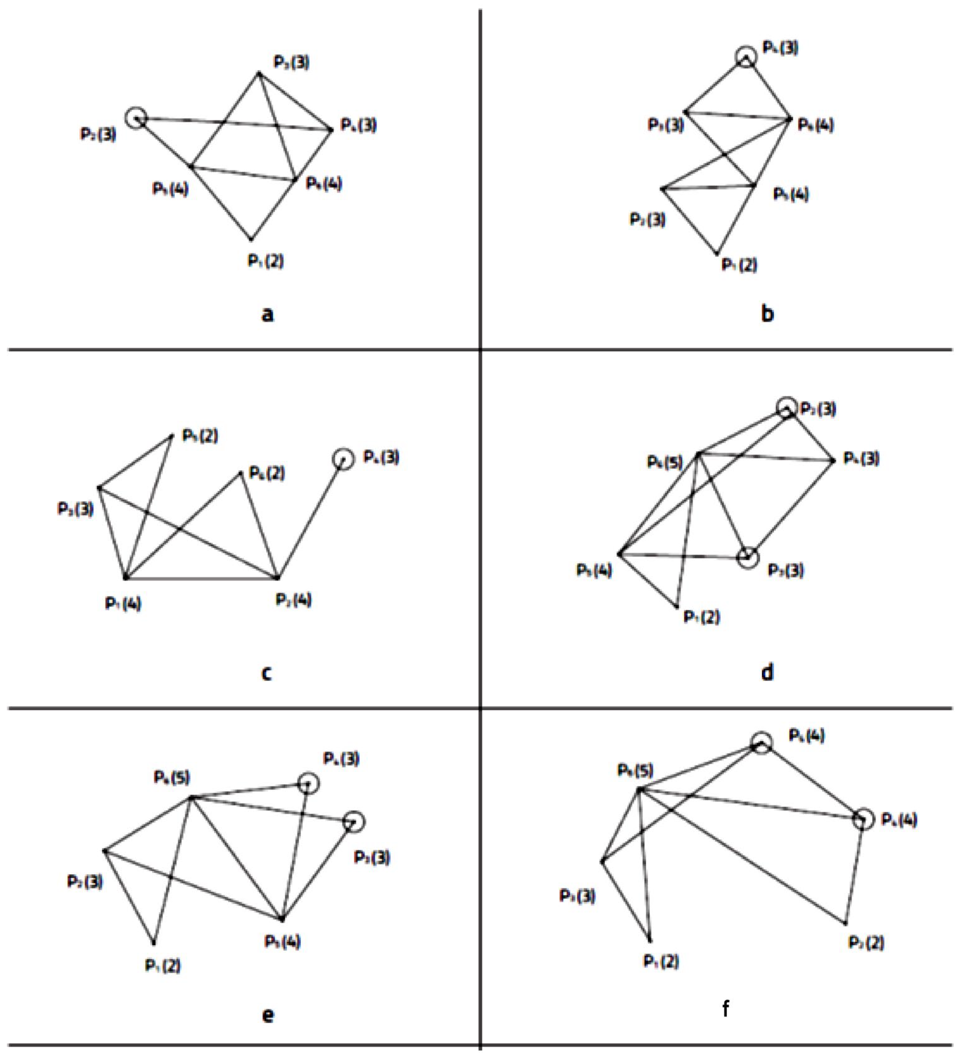
Now P₅(2) and P₆(2) cannot be connected according to theorem 8. Hence according to axiom d at least one of the vertices having V = 2, say P₅(2), must be connected to P₃(3) (The mediator between P₅(2) and P₁(4) must be one of the vertices already connected to P₁(4) as all its connections are already allocated. It cannot be P₆(2) due to Theorem 8 and it cannot be P₂(4) which has only one V = 2 vertex in its SS structure and this is P₆(2)). Since P₂(4) is connected to P₄(3) (circled in the figure), then according to axiom d they both have to be connected to their mediator, but this is impossible since the structure includes already six vertices and all the other vertices, except P₄(3), are fully connected in accordance with their valence.

We see then that the attempt to design an OS satisfying the above-mentioned conditions (m₂ = m₃ = m₄ = 2) results in contradiction.

Case B.

m₅ = 1.

In this case, m₄ ≤ 2 (Theorem 7). Also, m₂ ≤ 2 because the only possible SSs for the vertex having V = 2 are 5,4 and 5,3 (since these vertices must be connected to the vertex having V = 5, and according to Theorem 8, they cannot be connected to each other). Hence, if m₄ = 0, then m₂ = 1, and according to Theorem 3, m₃ = 4. But this result is impossible since, according to Theorems 10 and 12, there are only two possible SSs for the vertices having V = 3; SS = 5,3,3; and SS = 5,3,2. Hence, m₄ ≠ 0, so that m₄ = 1,2.

Let us show now that m₂ ≠ 0. Suppose that m₂ = 0, since m₄ ≤ 2 (Theorem 7) and m₃ + m₄ + 1 = 6 (Theorem 3) -> m₃ = 5 − m₄; then, m₃ ≥3. The only possible SSs for the vertex having V = 3 are 5,3,3; 5,4,3; and 5,4,4. But the case where SS = 5,3,3 is impossible. To show this, let us try to form an OS satisfying this condition. Let V(P₁) = 3 and SS(P₁) = 5,3,3. Let P₁ be connected to P₂, P₃, and P₄, where V(P₂) = 3, V(P₃) = 3, and V(P₄) = 5. P₂ and P₃ have to be connected to P₄ (having V = 5). Since V(P₂) = 3, and it is connected only to two vertices (P₁ and P₄), it has to be connected to an additional vertex, P₅ (not to P₃ because, in this case, SS(P₃) = 5,3,3, the same as SS(P₁)), and P₅ has to be connected to P₄. By the same token, P₃ and P₄ have to be connected to P₆. Now, the only possible values of the V of P₅ and P₆ is 4 (since m₂ = 0, and there are already three vertices having V = 3 and one vertex having V = 5). Therefore, SS(P₂) = SS(P₃) = 3,4,5. Hence, P₂ = P₃, in contradiction to axiom e.

We are left then with the following four possibilities: m₂ = 1,2 and m₄ = 1,2. For each of these cases, m₃ = 5 − m₂ − m₄, as ${3 \mathrm{m}}_3{+5 \mathrm{m}}_{5 }=\mathrm{even}.$ It follows for ${\mathrm{m}}_{5 }=1$ that

$$3 {\mathrm{m}}_3=\mathrm{even}-5=\mathrm{odd}$$

Thus, ${\mathrm{m}}_3 \ne 2$. The remaining cases are given in

Table 7. The possible multiplicities of the V = 2,3,4.

V = 2	V = 3	V = 4
1	3	1
2	1	2

.

We subsequently show that the attempt to design an OS satisfying the conditions of each row in this table always results in the contradiction of one of the axioms, a to e. Pay attention to the fact that, in all the cases discussed below, all the vertices have to be connected to P₆(5).

Let us begin with the first row of Table 7, in which m₂ = 1, m₃ = 3, m₄ = 1, and m₅ = 1. Let us denote the vertices of the possible OS by P₁(2), P₂(3), P₃(3), P₄(3), P₅(4), and P₆(5). (The numbers in parentheses are the valences of the vertices). The possible SSs of P₁(2) can be either SS = 4,5 or SS = 3,5. Let us discuss each of these cases separately.

Case 1.

SS(P₁(2)) = 4,5.

In this case (see Figure 5d), P₁(2) is connected to P₅(4) and P₆(5). Then, P₅(4) is connected to P₂(3), P₃(3), and P₆(5). Now, P₂(3) and P₃(3) have two connections (to P₅(4) and P₆(5)) instead of three, and the only available connection is to a vertex having V = 3. But such connections will yield that the SS of these vertices (circled in the figure) will be SS = 3,4,5, so that these two vertices will be equal, in contradiction to axiom e.

Case 2.

SS(P₁(2)) = 3,5.

In this case (see Figure 5e), P₁(2) is connected to P₂(3) and P₆(5). Then, P₅(4) is connected to P₂(3), P₃(3), P₄(3), and P₆(5). (As noted earlier, all the vertices have to be connected to P₆(5).) As a result, all the vertices are fully connected in accordance with their V, except the vertices having V = 3. P₃(3) and P₄(3) are circled in the figure. They each have only two connections instead of three. Trying to form a connection between these vertices will result in making them equal (they will both have SS = 3,4,5), in contradiction to axiom e.

The analysis of these two cases shows that it is impossible to design an OS satisfying the conditions of the first row of Table 7.

Let us examine now the second row in which m₂ = 2, m₃ = 1, m₄ = 2, and m₅ = 1. Let us denote the vertices of the possible OS by P₁(2), P₂(2), P₃(3), P₄(4), P₅(4), and P₆(5)—see Figure 5f. The possible SSs of P₁(2) and P₂(2) are, respectively, SS = 3,5, and SS = 4,5 since, as was indicated previously, they cannot be connected to each other. Hence, P₁(2) has to be connected to P₃(3) and P₆(5), and P₂(2) has to be connected to P₄(4) and P₆(5). At this stage, P₅(4) has only two connections (to P₆(5) and to P₄(4)), and it cannot be connected to P₁(2) and P₂(2), which do not have any more available connections. Therefore, only P₃(3) is available for connection. Hence, P₅(4) and P₄(4) (circled in the figure) each have only three connections instead of four. Hence, it is impossible to design an OS satisfying the conditions of the fourth row. □

Remark 1.

We described two OSs of order 7 in Section 2—O₁(7) and O₂(7)—satisfying the axioms of apriorics. There may be other OSs of order 7. The enumeration of all the OSs of order 7 and of higher orders is still an open problem in apriorics.

4. Properties of the Vertices of OS Graph

4.1. Introduction

In this section, we propose the notion of specifying properties to the nodes of the ontological structure (graph) determined uniquely by the nodes to which they are joined. This is demonstrated by analyzing the property combinations of the FE’s corresponding to the nodes of O₁(7) and O₂(7), which are discussed in Section 2.

How can the properties of a node (FE) be defined through its connections to the other nodes? According to the intuitive meaning of the relationship between the concept of a common property of two vertices and their connection, we can stipulate the following rules:

(a)

If two connected nodes in an ontological structure, V₁ and V₂, have a common property, f, then their mediator vertex connected to V₁ and V₂ (obligatory by axiom d) will be assigned the property f^ (complementary property).

Remark: The empirical meaning of f^ is that it facilitates the detection of f.

(b)

Two nodes of an ontological structure are joined if and only if either they have at least a common single property or one node has a complementary property of the other node.

(c)

A node in an ontological structure cannot have both a property and its complementary.

(d)

The set of properties of every node in an ontological structure must differ in at least a single property from the set of properties of any other node which is part of the same ontological structure.

Remark 2.

This rule is derived from axiom e, which requires that every two nodes be different.

4.2. Example: Intrinsic Properties of the Nodes of O₁(7) and O₂(7)

Following the rules specified above, the properties of the nodes belonging to O₁(7) are as follows: (a) The first property, f₁, is assigned to the fundamental entity P₁, as shown in Figure 6. (b) Since P₂ is not joined to P₁, it cannot be given the same property, so that we assign to it the different property, f₂. (c) P₄ is not joined to P₁ or to P₂. Thus, an additional property, f₃, is obligatory for its depiction. (d) P₅ is joined to P₂ and P₄ so that it possesses their complementary properties, denoted as f₂^ and f₃^. Thus, we should note that there is freedom in this assignment of properties according to the rules elaborated above. However, this freedom will not affect the conclusions. (e) P₇ is joined to P₁ and P₂ so that it is depicted by f₁ and f₂. Following the same procedure, we assign properties to other nodes, as clarified in Figure 6.

We observe that the minimal number of properties necessary for the ontological structure O₁(7) is three. It can easily be demonstrated that this prediction is valid also for O₂(7). The properties of O₂(7) nodes are specified by g₁, g₂, and g₃. To each of these properties, there is a complementary property, i.e., g₁^, g₂^, and g₃^.

Table 8. Properties of the vertices of O₁(7).

	Properties
P1	f1
P2	f2
P3	f1^,f3
P4	f3
P5	f2^,f3^
P6	f1^,f2^,f3^
P7	f1,f2

and Figure 6 give the properties of the nodes of O₁(7), and

Table 9. Properties of the vertices of O₂(7).

Vertex	Properties
Q1	g1
Q2	g2
Q3	g3
Q4	g1^,g3
Q5	g2^,g3^
Q6	g1^,g3^
Q7	g1,g2,g3

and Figure 7 give those of the nodes of O₂(7).

Apriorics predicts the three basic interactions corresponding to the three properties given in Table 8. This derivation is compatible with the existence of three fundamental interactions—electromagnetic, nuclear strong, and nuclear weak. These interactions bind the fundamental entities, thus forming the elementary and more complex particles.

Using Table 8, it is possible to give properties to the twelve binary compounds of O₁(7) that are the twelve fermion elementary particles of the standard model. This mapping enables the classification of these particles according to their properties. These predictions of apriorics do not contradict the known empirical standard model of particle physics.

Using Table 9, it is also possible to assign properties to the thirteen binary compounds of O₂(7) that are mapped to the thirteen known mediator particles (gauge bosons) that transfer the interaction between twelve elementary fermions. This designation enables the classification of these thirteen particles according to their properties. This prediction is again not contradicted by known empirical data [36].

5. Discussion: OS Graphs Used for Displaying Coreless Languages

In this paper, we described and analyzed a specified undirected simple OS graph and used it for the investigation of the fundamental entities and elementary and composite particles. We believe that these graphs can also be used in the holistic theory of knowledge [45,46] expressed in a certain language in which the meaning of every word and sentence is specified by the way it is joined to other words and sentences. Thus, it can be displayed as a graph of interconnected nodes corresponding to these words and sentences. Such a graph will have “core words” and “core sentences”, whose interpretation and truth are decided by elements which are beyond language. In our daily language, we have a multitude of core words representing objects existing in the real world. In the language used in empirical sciences, there exist a significant number of core sentences that have meaning dependent on observations and experiments. Mathematical theories depend on a core of fundamental notions joined via axioms whose justification lies externally. In each and every language, the core words and core sentences serve as means for specifying meaning to the other words and sentences of the language.

Can we contemplate a language without a core? Is it possible to imagine a language in which the meaning of its words (and sentences) will be specified solely by their interconnections?

We believe that the ontological structure is appropriate for displaying such a language, and the seven vertices of O₁(7) and O₂(7) can be thought of as the fundamental words in these simplest possible languages. The compounds of these nodes, which can be characterized by their properties, represent complex words and sentences.

In fact, every OS of order n represents a coreless language, including n basic words whose significance is derived solely from their interconnections. The compounds of these vertices define composite words and sentences in this language.