Statistical Analysis of the Negative–Positive Transformation in Image Encryption

Abstract

The negative–positive transformation (NPT) is a widely employed technique for encrypting images on pixel blocks, commonly integrated into cryptosystems compatible with compression algorithms. The existing literature on NPT analysis can be categorized into two types: theoretical analyses with results that apply to any image, primarily focused on compression compatibility, and numerical analyses that report empirical results from specific images, some without explaining the causes of the security results, while others are only related to the compression performance. Consequently, there is a significant gap in understanding the implications of applying the NPT for data protection. For that reason, this paper conducts a theoretical statistical analysis, presenting, demonstrating, and verifying six theorems to understand the security contributions of NPT. Two theorems examine the shape of the image histogram and the scatter plot of adjacent pixels after the NPT application. The subsequent four theorems explore the influence of NPT on the mean, variance, covariance, and correlation within each pixel block. The findings indicate that the NPT generates images with symmetrical histograms, the correlation of pixel blocks remains invariant, and distinct vertical and horizontal reflections manifest on the scatter plot. These theorems are verified by encrypting the Lena image with four pixel-block sizes. The histogram symmetry passed the goodness-of-fit test at a significance level of 5%, revealing consistent results. The correlation of pixel blocks remained unchanged, and the scatter plot exhibited an x-shaped pattern. Therefore, as the NPT alone does not achieve desirable encryption results, such as uniform histograms, scatter plots, and decreasing correlation, cryptosystems should complement it with additional techniques.

1. Introduction

The negative–positive transformation (NPT) is a commonly utilized encryption operation for securing images, particularly in compatible cryptosystems with compression techniques [1,2]. Notably, the NPT is employed in the encryption scheme of JPEG images, featuring prominently in various proposals [3,4,5,6,7]. In all of these instances, the NPT operates at the pixel block level [8] and applies to both color and grayscale images [9,10]. Moreover, the NPT finds applications beyond JPEG image encryption, extending its utility to hybrid methods like compressed sensing. In such applications, the NPT plays a role in achieving effective results for compressing encrypted images, as it can mask the original image before compression [11]. In addition, the versatility of the NPT is established in video encryption, particularly in MJPEG files [12]. In this context, it can replace video blocks within the original frames.

In its essence, the NPT finds application in the realm of data protection [13]. For instance, it is utilized to generate learnable transformed images, subsequently employed in convolutional neural network models. The objective is to control access to trained models [14]. Furthermore, various adaptations and versions based on the NPT have been developed. These proposals often strike a balance between security levels and the efficiency of compression savings [15]. One example is the injected negative–positive transformation (NINPT) [16] designed for compressed sensing. It is integrated into the encoding process to resist known plain-text attacks. Another variant is the double negative–positive transformation (DNPT) [17], which applies the NPT twice to encrypt images from a pixel matrix.

On the other hand, evaluating the security of algorithms designed to protect data is of paramount importance [18]. For image encryption algorithms, various measures and analyses are employed. One crucial aspect involves statistical analysis, often incorporating tools such as histograms, correlation assessments, and scatter plots [19,20]. The histogram illustrates the distribution of intensity levels among encrypted pixels in an image. Additionally, the histogram of the encrypted image is ideally uniform [21,22]. In cryptography, the goal is to introduce disparities between the original pixel values and the encrypted ones. The more evenly distributed the pixel values are, the more resilient the algorithm is against statistical attacks [23]. The correlation coefficient measures the relation between pixel values. Frequently, plain digital images tend to exhibit high correlation among adjacent pixels, capturing image features in specific regions [24]. In this way, the scatter plot is part of correlation analysis, plotting pairs of adjacent pixels to visualize the distribution of correlation in a specific direction [25].

However, the scope of analyses related to the NPT is limited, classifiable into theoretical and numerical works, where the former yields results applicable to any image, and the latter provides outcomes specific to certain images. The existing theoretical analyses primarily explore the relationship between pixels after NPT encryption. For instance, one study focuses on the Euclidean distance and the inner product of pixel vectors [26], aiming to assess image compatibility with machine learning models. In contrast, our work evaluates the NPT effects on the image histogram to analyze its statistical security. Other theoretical analyses in the EtC domain concentrate on preserving image properties for an effective compression process [27]. Differing from these theoretical analyses focused on preserving compatibility, ours is grounded in security considerations.

In the realm of numerical analysis, studies address security concerns related to encryption quality, using statistical parameters such as the correlation coefficient. However, these analyses are numerical and specifically reported from certain images [28], in contrast to the theorems presented in this study, which have applicability to any image. While other works mention that each pixel block in images encrypted with EtC exhibits almost the same correlation as the original images [29,30], they lack a demonstration of the underlying causes, a gap addressed in our work. Moreover, a comprehensive statistical analysis is often absent in this genre of research, which typically focuses solely on compression results [31]. Hence, our proposed study emphasizes a security analysis. Understanding the security implications of the NPT is crucial, particularly as it serves as the final step in some cryptosystems [32], and its outcomes can directly impact the encrypted information.

Therefore, it is necessary to explore the contribution of the NPT to the cryptosystem’s security. This paper theoretically analyzes the NPT through one of the most essential studies: statistical analysis. Within this analysis, six theorems are presented, each accompanied by its respective demonstration and subsequently validated through computer simulations.

1.1. Motivation

Given the regular application of the NPT in encryption schemes compatible with compression, there is a need to explore its individual security performance. Existing security analyses are limited, and other studies primarily concentrate on compression performance. To understand the limitations of the technique, it is crucial to move beyond a mere numerical study and conduct a theoretical analysis. An individual analysis of the NPT can offer insights into its specific contribution to security. This knowledge is essential for the design of new encryption techniques aimed at enhancing results in encryption and compression schemes and complementing the application of the NPT with other procedures.

1.2. Contribution

The primary contribution of this work lies in the security study of using the NPT for image encryption through a theoretical statistical analysis. Six theorems are presented to elucidate various statistical outcomes after the application of the NPT. Two theorems examine the shape of the image histogram and the scatter plot of adjacent pixels. The remaining four theorems delve into the impact of NPT on the mean, variance, covariance, and correlation within each pixel block. In addition to the theoretical demonstration of these theorems, their computational verification is carried out by encrypting the Lena image using NPT. The results obtained can be leveraged in the development of future encryption techniques and implementations of NPT in cryptosystems to enhance security considerations.

The paper’s organization is as follows. Section 2 presents the main concepts of this work, the NPT, correlation coefficient, binomial distribution, and the goodness of fit test. Section 3 contains the theoretical statistical analysis of the NPT encryption, presenting the six theorems and their proofs. Section 4 consists of the encrypted images, graphs, and tables that verify the theorems. Section 5 and Section 6 are the discussion and conclusions sections.

2. Materials and Methods

The encryption-then-compression (EtC) systems, which incorporate block scrambling, encrypt an image with dimensions $W=M\times N$ pixels in blocks of size $w=m\times n$ pixels, where M indicates the number of pixel rows in the image, N denotes the number of pixel columns, and W represents the total number of pixels in the image. Similarly, in the pixel block, m indicates the number of pixel rows, n denotes the number of pixel columns, and w denotes the number of pixels in the block. This scheme incorporates the NPT as one of the techniques within the EtC systems, as depicted in Figure 1. The NPT is applied to pixel blocks and all color components of the pixels.

2.1. The Negative–Positive Transformation

The negative–positive transformation (NPT) is an encryption technique applied per pixel block, selectively transforming some pixel color values while leaving others unaltered. The NPT randomly employs the XOR binary operation between the pixel color value $px\left(i\right)$ and the number 255. The number 255 corresponds to the case where the number of intensity levels of a pixel color value is equal to 256. The decision to change the pixel color value, $px\left(i\right)$, to $p{x}^{\prime }\left(i\right)=px\left(i\right)\oplus 255$ or retain its original value, $p{x}^{\prime }\left(i\right)=px\left(i\right)$, is determined by a discrete random variable, X. In summary, the NPT application is defined by Equation (1). It is necessary to note that this transformation is applied to each pixel block, a, of the image, affecting all pixel color values $px\left(i\right)$ within the block, a, where $1\le a\le W/w$ and $1\le i\le w$.

$$p{x}^{\prime }\left(i\right)=\left\{\begin{array}{cc}px\left(i\right)\oplus 255,\hfill & \mathrm{if}X=1\hfill \\ px\left(i\right),\hfill & \mathrm{if}X=0\hfill \end{array}\right.$$

(1)

It is important to note that the variable X is a Bernoulli discrete random variable (BDRV), as defined in Equation (2). The probability mass function for X is presented in

Table 1. Probability mass function of X in tabular form.

x	0	1
$p\left(x\right)$	0.5	0.5

.

$$X=\left\{\begin{array}{cc}1,\hfill & \mathrm{if}\mathrm{the}\mathrm{pixel}\mathrm{block}a\mathrm{is}\mathrm{selected}\hfill \\ 0,\hfill & \mathrm{if}\mathrm{the}\mathrm{pixel}\mathrm{block}a\mathrm{is}\mathrm{not}\mathrm{selected}\hfill \end{array}\right.$$

(2)

Additionally, it is noteworthy that Equation (1) can be expressed as Equation (3), as the XOR operation can be interpreted as the two’s complement of an 8-bit number, which represents values between 0 and 255.

$$p{x}^{\prime }\left(i\right)=\left\{\begin{array}{cc}255-px\left(i\right),\hfill & \mathrm{if}X=1\hfill \\ px\left(i\right),\hfill & \mathrm{if}X=0\hfill \end{array}\right.$$

(3)

In summary, an initial random number, $X=x$, is generated for each pixel block encryption. Subsequently, the computation of $p{x}^{\prime }\left(i\right)$ takes place for all pixels within the same pixel block according to the generated number. The process applies to each color channel, c, in the case of a color image. Below are two examples illustrating the implementation of the NPT for a color image, where each pixel, i, has three color components, $px\left(i\right)=\{R_i,G_i,B_i\}$.

Table 2. The Negative-Positive Transformation (NPT) application over a color-pixel block of $w=3$ pixels and $X=1$.

	First Pixel			Second Pixel			Third Pixel
Value	${\mathbf{R}}_{\mathbf{1}}$	${\mathbf{G}}_{\mathbf{1}}$	${\mathbf{B}}_{\mathbf{1}}$	${\mathbf{R}}_{\mathbf{2}}$	${\mathbf{G}}_{\mathbf{2}}$	${\mathbf{B}}_{\mathbf{2}}$	${\mathbf{R}}_{\mathbf{3}}$	${\mathbf{G}}_{\mathbf{3}}$	${\mathbf{B}}_{\mathbf{3}}$
$px\left(i\right)$	120	254	31	123	252	37	118	249	34
$p{x}^{\prime }\left(i\right)$	135	1	224	132	3	218	137	6	221

corresponds to the example when the random number is $X=1$, and

Table 3. The NPT application over a color-pixel block of $w=3$ pixels and $X=0$.

	First Pixel			Second Pixel			Third Pixel
Value	${\mathbf{R}}_{\mathbf{1}}$	${\mathbf{G}}_{\mathbf{1}}$	${\mathbf{B}}_{\mathbf{1}}$	${\mathbf{R}}_{\mathbf{2}}$	${\mathbf{G}}_{\mathbf{2}}$	${\mathbf{B}}_{\mathbf{2}}$	${\mathbf{R}}_{\mathbf{3}}$	${\mathbf{G}}_{\mathbf{3}}$	${\mathbf{B}}_{\mathbf{3}}$
$px\left(i\right)$	10	41	55	19	42	53	11	37	54
$p{x}^{\prime }\left(i\right)$	10	41	55	19	42	53	11	37	54

corresponds to the case when the generated number is $X=0$. In both scenarios, the number of pixels, w, in the block is equal to 3. The original pixel values for Example 1 are $px\left(1\right)=\{120,254,31\}$, $px\left(2\right)=\{123,252,37\}$, and $px\left(3\right)=\{118,249,34\}$, while for Example 2, the values are $px\left(1\right)=\{10,41,55\}$, $px\left(2\right)=\{19,42,53\}$, and $px\left(3\right)=\{11,37,54\}$.

2.2. Correlation Coefficient

The correlation coefficient ($\rho$) assesses the confusion and diffusion effects in an encrypted image by considering pairs of pixels [34]. It is defined by Equation (4). In this context, let K represent the discrete random variable for the pixel color value in the original image, and Q denote the adjacent pixel color value in the original image. Throughout this work, the samples consist of w pixels as elements, where the total number of pixels in an image is W, and $w\le W$.

$$\rho (K,Q)=\frac{\mathrm{Cov}(K,Q)}{\sqrt{\mathrm{Var}\left(K\right)}\sqrt{\mathrm{Var}\left(Q\right)}}$$

(4)

where the covariance Cov$(K,Q)$, applicable to image encryption [35,36], is shown in Equation (5). It serves as a measure to evaluate the strength of the relationship between two random variables, K and Q.

$${\displaystyle \mathrm{Cov}(K,Q)=\frac{1}{w}\sum _{i=1}^w(k_i-\overline{k})(q_i-\overline{q})}$$

(5)

Also, variance $s_k^2$ or Var$\left(K\right)$ of a sample is defined in Equation (6).

$${\displaystyle \mathrm{Var}\left(K\right)=\frac{1}{w}\sum _{i=1}^w{(k_i-\overline{k})}^2}$$

(6)

Finally, the mean $\overline{k}$ of a sample with w elements is defined in Equation (7).

$${\displaystyle \overline{k}=\frac{1}{w}\sum _{i=1}^w{k}_i}$$

(7)

2.3. Binomial Distribution

If a distribution is binomial, the following conditions must be satisfied [37]:

• It has a fixed number of trials n.
• In each trial, there are two possible outcomes.
• One outcome is termed as a success with a fixed probability, p, for all the trials.
• The trials are independent of each other.
• The random variable Y denotes the number of successes observed after the n-executed trials.

If all the aforementioned conditions are met, the probability mass function for the variable Y is given by Equation (8). In addition, if Y follows a binomial distribution, it can be denoted as $Y\sim \mathrm{B}(n,p)$.

$$f_Y(n,p)=\left(\genfrac{}{}{0pt}{}{n}{y}\right)p^y{(1-p)}^{n-y}$$

(8)

where $y=0,1,2,3,\cdots ,n$, its expected value is $E\left[Y\right]=np$, and the variance is Var$\left(Y\right)=np(1-p)$.

2.4. Goodness-of-Fit Test

It is a statistical hypothesis test used to compare if the observed data from a sample of d elements has an expected distribution. In other words, it assesses the fit of the theoretical distribution with the collected information [38]. The test is based on proving the null hypothesis, $H_0:$ The data follow the theoretical distribution. Although not rejecting $H_0$ should not be interpreted as accepting it as verified. The traditional goodness-of-fit test follows the chi-square test. It works with the ${\chi }^2$ statistic, computed as Equation (9) defines it. It sums the squared deviations between the observed registers, $O_i$, and the expected values, $E_i$.

$${\displaystyle {\chi }^2=\sum _{i=1}^d\frac{{(O_i-E_i)}^2}{E_i}}$$

(9)

The ${\chi }^2$ has $d-1$ degrees of freedom, where d indicates the number of categories (cells) into which the data are divided [39]. Additionally, the statistical test has an associated p-value. Specifically, a histogram of 256 classes follows a theoretical distribution if ${\chi }^2<291$ with a significance level of $0.05$ [40]. The preceding information is relevant since the color images in this work have 256 different intensity levels.

3. Statistical Analysis

In this section, the statistical analysis is conducted through the presentation and proof of six theorems. Section 3.1 contains the theorem on the histogram. Section 3.2 provides the theorem on the mean, Section 3.3 presents the theorem on variance, and Section 3.4 addresses the theorem on covariance. Section 3.5 explores the theorem on correlation. Finally, Section 3.6 delves into the theorem on the scatter plot. The theorems on the histogram and scatter plot encompass the results of the entire image, while the remaining theorems focus specifically on the outcomes of pixel blocks. Furthermore, Section 3.3, Section 3.4 and Section 3.5 include two distinct proofs each.

The analysis is based on the following assumptions. Firstly, considering that the NPT in EtC systems is implemented in the RGB space, the analysis focuses specifically on this color space. Furthermore, NPT operates by pixel block; hence, the results derived from the analysis apply to pixel-block encryption. Also, it is assumed that the image width is a multiple of the block width, and the image height is a multiple of the block height. While the current examination is conducted on a single color component, it is important to note that the findings can be extrapolated to any of the three colors in the RGB space. Subsequently, the upcoming section will perform computer verification for each color, aligning with the outcomes of this theoretical analysis.

3.1. Histogram

Histograms applied to images serve to depict the frequency distribution of each color intensity across all pixels. In other words, it quantifies the number of pixels with a specific intensity value throughout the entire image. This process is replicated for each color channel, providing statistical insights into its distribution [41]. In the present study, the number of intensity levels is 256, ranging from 0 to 255, and there are three colors: red, green, and blue. However, it does not capture information about the spatial position of individual pixels. Following the application of the NPT procedure, the new pixel color values, $p{x}^{\prime }\left(i\right)$, lead to a redistribution of the original intensity levels within the image histogram. In this context, the resulting frequencies of the histogram are analyzed in Theorem 1.

Theorem 1.

The intensity level distribution of any image, after applying the NPT, conforms to a symmetric histogram.

Proof. 

The proof involves two probabilistic experiments to examine the modified distribution.

• Observe the new pixel color value, $p{x}^{\prime }\left(i\right)$, after the NPT, of a pixel with an original color value equal to h. This analysis applies to all instances of $px\left(i\right)=h$.
• Observe the new pixel color value, $p{x}^{\prime }\left(i\right)$, after the NPT, of a pixel with an original color value equal to $h\oplus 255$. It is repeated for all instances of $px\left(i\right)=h\oplus 255$.

Therefore, the observation in experiment number 1 has two possibilities: retaining its value as $p{x}^{\prime }\left(i\right)=h$ or modifying it to $p{x}^{\prime }\left(i\right)=h\oplus 255$. In this context, the BDRV, $S_i$, is defined in Equation (10) to represent this scenario. Additionally, in experiment two, there are two possibilities, and to signify them, the BDRV, $T_i$, is defined in Equation (11).

$$S_i=\left\{\begin{array}{cc}1,\hfill & \mathrm{if}p{x}^{\prime }\left(i\right)=h\hfill \\ 0,\hfill & \mathrm{if}p{x}^{\prime }\left(i\right)=h\oplus 255\hfill \end{array}\right.$$

(10)

$$T_i=\left\{\begin{array}{cc}1,\hfill & \mathrm{if}p{x}^{\prime }\left(i\right)=h\hfill \\ 0,\hfill & \mathrm{if}p{x}^{\prime }\left(i\right)=h\oplus 255\hfill \end{array}\right.$$

(11)

It is important to note that in Equation (11), value h is obtained when $px\left(i\right)=h\oplus 255$ changes its value to $p{x}^{\prime }\left(i\right)=(h\oplus 255)\oplus 255=h$. Additionally, considering the NPT composition in Equation (1), the probabilities for both $S_i$ and $T_i$ variables are $p\left(0\right)=p\left(1\right)=0.5$.

Another point to consider is that experiment number 1 can only be executed over the $l_h\le W$ pixel color values, such that $px\left(i\right)=h$, and similarly, the second experiment can be performed $l_{h\oplus 255}$ times. Consequently, two new discrete random variables are defined, $S_{\mathrm{tot}}$ and $T_{\mathrm{tot}}$, corresponding to the sum of the variables, $S_i$ and $T_i$, respectively. Both are presented in Equations (12) and (13).

Additionally, considering that the sum of BDRV converges to a binomial distribution [42], it follows that $S_{\mathrm{tot}}\sim B(l_h,0.5)$, where the number of trials is $l_h$, and the probability of success is equal to $0.5$. Similarly, $T_{\mathrm{tot}}\sim B(l_{h\oplus 255},0.5)$, with $l_{h\oplus 255}$ trials and a success probability of $0.5$.

$${\displaystyle S_{\mathrm{tot}}=\sum _{i=1}^{l_h}{S}_i}$$

(12)

$${\displaystyle T_{\mathrm{tot}}=\sum _{i=1}^{l_{(h\oplus 255)}}{T}_i}$$

(13)

In other words, the variable $S_{\mathrm{tot}}$ corresponds to the number of transformed pixels $p{x}^{\prime }\left(i\right)=h$, such that the pixel color component was previously $px\left(i\right)=h$. Similarly, the variable $T_{\mathrm{tot}}$ represents the number of $p{x}^{\prime }\left(i\right)=h$ occurrences, which was previously $px\left(i\right)=h\oplus 255$.

Furthermore, it can be verified that both variables satisfy the conditions for a binomial distribution. For example, the verification for the variable $S_{\mathrm{tot}}$ is provided below.

• It has a fixed number of trials $l_h$, which is the original number of pixels that satisfy $px\left(i\right)=h$.
• There are only two possible outcomes: $p{x}^{\prime }\left(i\right)=h$ and $p{x}^{\prime }\left(i\right)=h\oplus 255$.
• The success is $p{x}^{\prime }\left(i\right)=h$ with a probability of $p=0.5$.
• The trials are independent because, within a pixel block, there are similar pixel color values, though not necessarily the same. Then, the NPT is applied independently to each pixel $px\left(i\right)=h$.

On the other hand, a final discrete random variable is proposed, denoted as F, representing the number of color pixels with a value equal to h after the NPT. It is defined in Equation (14) and can be replicated for each color c.

$$F=S_{\mathrm{tot}}+T_{\mathrm{tot}}$$

(14)

With this in mind, the expected value of F is given in Equation (15).

$$E\left(F\right)=E(S_{\mathrm{tot}}+T_{\mathrm{tot}})=E\left(S_{\mathrm{tot}}\right)+E\left(T_{\mathrm{tot}}\right)$$

(15)

Since $S_{\mathrm{tot}}$ and $T_{\mathrm{tot}}$ follow a binomial distribution, their expected value is computed as $n\times p$, resulting in Equation (16). This represents the number of pixel color values equal to h after the NPT.

$$E\left(F\right)=l_h\times 0.5+l_{h\oplus 255}\times 0.5=\frac{(l_h+l_{h\oplus 255})}{2}$$

(16)

Now, to estimate the number of pixel color values equal to $h\oplus 255$ after the NPT, the variables $S_{\mathrm{tot}}^{\prime }$ and $T_{\mathrm{tot}}^{\prime }$ are defined in Equations (17) and (18), respectively. Here, $S_{\mathrm{tot}}^{\prime }$ represents the number of transformed pixels $p{x}^{\prime }\left(i\right)=h\oplus 255$ that were originally $px\left(i\right)=h$. Meanwhile, $T_{\mathrm{tot}}^{\prime }$ considers the number of transformed pixels $p{x}^{\prime }\left(i\right)=h\oplus 255$ with the original color values $px\left(i\right)=h\oplus 255$.

$$S_{\mathrm{tot}}^{\prime }=l_h-S_{\mathrm{tot}}$$

(17)

$$T_{\mathrm{tot}}^{\prime }=l_{h\oplus 255}-T_{\mathrm{tot}}$$

(18)

Thus, the variable $F^{\prime }$, as defined in Equation (19), represents the frequency of the $h\oplus 255$ level after the NPT.

$$F^{\prime }=S_{\mathrm{tot}}^{\prime }+T_{\mathrm{tot}}^{\prime }$$

(19)

Now, the expected value of $F^{\prime }$, indicating the expected frequency of pixel color values equal to the $h\oplus 255$ level, is shown in Equation (20).

$$E\left(F^{\prime }\right)=E(S_{\mathrm{tot}}^{\prime }+T_{\mathrm{tot}}^{\prime })=E(l_h-S_{\mathrm{tot}}+l_{h\oplus 255}-T_{\mathrm{tot}})$$

(20)

The expected value can also be expressed as Equation (21) by rearranging and utilizing the definition of F in Equation (14).

$$E\left(F^{\prime }\right)=E(l_h+l_{h\oplus 255}-\left(S_{\mathrm{tot}+}{T}_{\mathrm{tot}}\right))=E(l_h+l_{h\oplus 255}-F)$$

(21)

Finally, the resultant $E\left(F\right)$ from Equation (16) leads to Equation (22).

$$E\left(F^{\prime }\right)=l_h+l_{h\oplus 255}-E\left(F\right)=l_h+l_{h\oplus 255}-\frac{(l_h+l_{h\oplus 255})}{2}$$

(22)

Simplifying the expected value of $F^{\prime }$, it is presented in Equation (23). This result is equivalent to the $E\left(F\right)$ obtained in Equation (16). In other words, the expected value of the number of frequencies for the color level h is the same as the color level $h\oplus 255$. This is anticipated for all the intensity levels of the histograms after applying the NPT.

$$E\left(F^{\prime }\right)=\frac{(l_h+l_{h\oplus 255})}{2}=E\left(F\right)$$

(23)

□

3.2. Arithmetic Mean

The mean $\overline{k^{\prime }}$ calculates the average of the new pixel color values $p{x}^{\prime }\left(i\right)$ after the NPT application to the w pixels within a pixel block. This is illustrated in Equation (24).

$${\displaystyle \overline{k^{\prime }}=\frac{1}{w}\sum _{i=1}^{w}p{x}^{\prime }\left(i\right)}$$

(24)

Theorem 2.

The mean of the pixels in a block after the NPT is equal to the NPT of its original mean.

Proof. 

The demonstration considers two cases: when the BDRV $X=1$, and $X=0$. In the former, the value $px\left(i\right)=k_i$ changes to $p{x}^{\prime }\left(i\right)=k_i\oplus 255$, while Equation (25) illustrates its mean $\overline{k^{\prime }}$.

$${\displaystyle \overline{k^{\prime }}=\frac{1}{w}\sum _{i=1}^w(255-k_i)}$$

(25)

Equation (25) is split into two sums, resulting in Equation (26).

$$\overline{k^{\prime }}=\frac{1}{w}\left({\displaystyle \sum _{i=1}^{w}255-\sum _{i=1}^w{k}_i}\right)$$

(26)

The first term is a constant sum, and the second one corresponds to Equation (7). The simplified result is in Equation (27).

$$\overline{k^{\prime }}=255-\overline{k}$$

(27)

Which is equivalent to Equation (28).

$$\overline{k^{\prime }}=\overline{k}\oplus 255$$

(28)

In the case of $X=0$, the pixel value remains unchanged, i.e., $p{x}^{\prime }\left(i\right)=px\left(i\right)$. Consequently, the mean also remains the same, $\overline{k^{\prime }}=\overline{k}$.

In conclusion, in both cases, the mean of pixels in a block after the NPT is equal to the NPT of its original mean, as shown in Equation (29).

$$\overline{k^{\prime }}=\left\{\begin{array}{cc}\overline{k}\oplus 255,\hfill & \mathrm{if}X=1\hfill \\ \overline{k},\hfill & \mathrm{if}X=0\hfill \end{array}\right.$$

(29)

□

3.3. Variance

Similarly to the mean, the variance of $p{x}^{\prime }\left(i\right)$ in a pixel block after applying the NPT is analyzed with Equation (6). Since the pixels might change their values, the mean $\overline{k^{\prime }}$ also needs to be considered (obtained in Equation (29)). Consequently, the variance $s_k^{\prime 2}$, which includes these considerations, is shown in Equation (30).

$${\displaystyle s_k^{\prime 2}=\frac{1}{w}\sum _{i=1}^w{(p{x}^{\prime }\left(i\right)-\overline{k^{\prime }})}^2}$$

(30)

The variance quantifies the degree of dispersion among the elements within a set [41]. It considers the squared distance between a specific value of the set and the mean of the set. It computes all the distances in this manner for all the elements of the set. Subsequently, their average is calculated to derive the variance. In this context, the set is the pixel block, and the elements are the pixel color values. Since the mean can change after the NPT application, the variance must consider this modification along with the encryption of the pixel color values. In this way, the Theorem 3 is presented.

Theorem 3.

The variance of pixels in a block remains invariant after the NPT.

Proof. 

The demonstration considers the two following NPT cases: $X=1$ and $X=0$. When $X=1$, then $p{x}^{\prime }\left(i\right)=255-k_i$, and the resulting variance $s_k^{\prime 2}$ is expressed in Equation (31), taking into account the mean from Equation (27).

$${\displaystyle s_k^{\prime 2}=\frac{1}{w}\sum _{i=1}^w{(255-k_i-(255-\overline{k}))}^2}$$

(31)

The simplified form of Equation (31) is presented in Equation (32).

$${\displaystyle s_k^{\prime 2}=\frac{1}{w}\sum _{i=1}^w{(-k_i+\overline{k})}^2}$$

(32)

Finally, it can be observed that Equations (6) and (32) are equivalent, both representing the same quadratic term.

$$s_k^{\prime 2}=s_k^2$$

(33)

In the case of $X=0$, where the pixel values remain unchanged ($p{x}^{\prime }\left(i\right)=px\left(i\right)$), the variance remains the same, i.e., $s_k^{\prime 2}=s_k^2$. In conclusion, the NPT does not alter the variance of any pixel block in either case. □

Proof. 

Another method to derive the variance result is through the proposition in Equation (34), which applies to linear functions of the form $aK+b$ [43].

$$\mathrm{Var}(aK+b)=a^2{\sigma }_K^2$$

(34)

Let the discrete random variable $K^{\prime }$ represent the pixel color value in the block after the NPT. When $X=1$, $K^{\prime }$ takes the value $255-K$. Therefore, applying the proposition, its resulting variance is given by Equation (35). In this case, $a=-1$ and $b=0$.

$$\mathrm{Var}\left(K^{\prime }\right)=\mathrm{Var}(-K+255)={(-1)}^2{s}_k^2=s_k^2$$

(35)

Consequently, the variance after the NPT application, whether $X=1$ or $X=0$, remains unchanged. □

3.4. Covariance

In a similar manner, the covariance is examined after the NPT by employing two discrete random variables. One is the variable $K^{\prime }$ introduced earlier in the variance section, and another random variable is defined as $Q^{\prime }:$ The adjacent pixel color value in the block after the NPT. The covariance of both variables is computed using Equation (5), resulting in Equation (36).

$${\displaystyle \mathrm{Cov}(K^{\prime },Q^{\prime })=\frac{1}{w}\sum _{i=1}^w(k_i^{\prime }-\overline{k^{\prime }})(q_i^{\prime }-\overline{q^{\prime }})}$$

(36)

The covariance measures the degree of the relationship between a pair of variables, denoted as $K^{\prime }$ and $Q^{\prime }$, within the same sample [41]. In this case, the sample is the pixel block, and the pairs of variables are defined by the values of adjacent pixels. Similar to the variance, the covariance assesses the distance of each variable value from its respective mean, and subsequently multiplies them. Consequently, the sign of the covariance depends on the variability of one variable relative to the other. A positive covariance indicates a change in the same direction, while a negative sign suggests an opposite change. Now, the relationship between these variables is assessed after the NPT application. In this context, the Theorem 4 is presented.

Theorem 4.

The covariance within a pixel block remains invariant after the NPT.

Proof. 

The NPT, in the case of $X=0$, preserves the initial covariance $\mathrm{Cov}(K^{\prime },Q^{\prime })=\mathrm{Cov}(K,Q)$, similar to the mean and variance. Conversely, when the NPT takes the value $X=1$, the alternative definition of the NPT in Equation (3) for $k_i^{\prime }$ and $q_i^{\prime }$, along with the sample mean value result of Equation (27), modifies Equation (36) to Equation (37).

$${\displaystyle \mathrm{Cov}(K^{\prime },Q^{\prime })=\frac{1}{w}\sum _{i=1}^w((255-k_i)-(255-\overline{k}))((255-q_i)-(255-\overline{q}))}$$

(37)

Simplifying, the result is presented in Equation (38).

$${\displaystyle \mathrm{Cov}(K^{\prime },Q^{\prime })=\frac{1}{w}\sum _{i=1}^w(-k_i+\overline{k})(-q_i+\overline{q})}$$

(38)

Consequently, the product can be expressed as shown in Equation (39).

$${\displaystyle \mathrm{Cov}(K^{\prime },Q^{\prime })=\frac{1}{w}\sum _{i=1}^w(-1)(k_i-\overline{k})(-1)(q_i-\overline{q})}$$

(39)

Therefore, the final result is shown in Equation (40).

$${\displaystyle \mathrm{Cov}(K^{\prime },Q^{\prime })=\frac{1}{w}\sum _{i=1}^w(k_i-\overline{k})(q_i-\overline{q})}$$

(40)

In conclusion, the NPT does not modify the covariance value in a pixel block.

$$\mathrm{Cov}(K^{\prime },Q^{\prime })=\mathrm{Cov}(K,Q)$$

(41)

□

Proof. 

Another approach to validate the covariance result is through the use of the proposition in Equation (42) [43].

$$\mathrm{Cov}(aK+c,Q)=a\mathrm{Cov}(K,Q)$$

(42)

In the NPT, when $X=1$, the discrete random variables $K^{\prime }$ and $Q^{\prime }$ change to $255-K$ and $255-Q$, respectively, as illustrated in Equation (43).

$$\mathrm{Cov}(K^{\prime },Q^{\prime })=\mathrm{Cov}(-K+255,-Q+255)$$

(43)

Therefore, we apply the preposition of Equation (42) to Equation (43) with $a=-1$ and $b=255$.

$$\mathrm{Cov}(K^{\prime },Q^{\prime })=(-1)\mathrm{Cov}(K,-Q+255)$$

(44)

Since $\mathrm{Cov}(K,Q)=\mathrm{Cov}(Q,K)$, applying Equation (42) once more yields Equation (45).

$$\mathrm{Cov}(K^{\prime },Q^{\prime })=(-1)(-1)\mathrm{Cov}(Q,K)$$

(45)

Consequently.

$$\mathrm{Cov}(K^{\prime },Q^{\prime })=\mathrm{Cov}(K,Q)$$

(46)

□

3.5. Pearson Correlation

The correlation of Equation (4) is rewritten as Equation (47) to denote the NPT application.

$$\rho (K^{\prime },Q^{\prime })=\frac{\mathrm{Cov}(K^{\prime },Q^{\prime })}{\sqrt{\mathrm{Var}\left(K^{\prime }\right)}\sqrt{\mathrm{Var}\left(Q^{\prime }\right)}}$$

(47)

Theorem 5.

The Pearson correlation in a pixel block remains invariant under the NPT.

Proof. 

Combining the results obtained for variance in Equation (33) and covariance in Equation (41), the overall result is presented in Equation (48).

$$\rho (K^{\prime },Q^{\prime })=\frac{\mathrm{Cov}(K,Q)}{\sqrt{\mathrm{Var}\left(K\right)}\sqrt{\mathrm{Var}\left(Q\right)}}$$

(48)

In conclusion, the correlation remains unaltered, i.e., $\rho (K^{\prime },Q^{\prime })=\rho (K,Q)$. □

3.6. Scatter Plot

Given two pixel values denoted as r and s, where one is adjacent to the other, their representation on a scatter plot can be with the point $(r,s)$. The NPT application shifts this point in horizontal and vertical directions, as depicted in Figure 2. It is important to highlight that reflections occur concerning the center at $(127,127)$.

Below, each of the reflections presented in Figure 2 are described as follows:

• Vertical reflection. In Figure 2b, the pixel value r remains unchanged after the application of the NPT, indicating that it was applied in this block with $X=0$. On the other hand, the adjacent pixel with an original value, s, changes its value to $255-s$, signifying that it belongs to another (but adjacent) pixel block where the NPT has been applied with $X=1$.
• Horizontal reflection. In Figure 2d, the pixel value r transforms to $255-r$ after the application of the NPT with $X=1$ in its block. Meanwhile, the adjacent pixel with value s belongs to another pixel block (though adjacent), and in that block, the NPT is applied with $X=0$, resulting in an unchanged value.
• Simultaneous vertical and horizontal reflection. This is illustrated in Figure 2c. In contrast to the other two cases, this type of reflection arises from two possibilities. Firstly, both adjacent pixels with values r and s are in the same pixel block, and the NPT is applied with $X=1$ in that pixel block. The second possibility is that both pixel values are in different pixel blocks, but in both blocks, the NPT is applied with $X=1$.

Theorem 6.

The NPT results in reflections in a scatter plot, occurring over either the horizontal, vertical, or both axes, with the point of origin set at $(127,127)$.

Proof. 

The demonstration evaluates the distance of the new point to the origin $(127,127)$ in various directions after applying the NPT compared to the original distances.

In the horizontal direction, let $d=|127-r|$ represent the distance to the center before the NPT. If the NPT, applied to its corresponding pixel, has $X=1$, then $d=|127-(255-r\left)\right|=|-128+r|=|128-r|$. Otherwise, it does not alter its value, and the distance remains unchanged.

Similarly, the distance to the center in the vertical direction is $d=|127-s|$. If it modifies its value, the distance becomes $d=|127-(255-s\left)\right|=|-128+s|=|128-s|$. □

4. Computer Verification

In this section, we validate the six theorems by implementing the NPT and applying it to encrypt the Lena image (Figure 3). Furthermore, the original histograms and scatter plots are displayed in Figure 4. As the NPT operates on pixel blocks, and although the theorems are demonstrated for any size, we present the results of four different block sizes. The encryption results in sizes of $2\times 2$, $4\times 4$, $8\times 8$, and $16\times 16$ are shown in Figure 5.

Concerning the execution time for encrypting the Lena color image of 512 × 512 pixels, it is 120.03 ms for a pixel block size of $2\times 2$, 82.05 ms for a size of $4\times 4$, 78.80 ms for a block size of $8\times 8$, and finally, 78.64 ms for a size of $16\times 16$.

4.1. Histogram

The histograms in Figure 5 display a symmetric shape, with the center around intensity levels of 127–128. Additionally, each color histogram is presented for the four different pixel block sizes. The red color histogram is depicted in Figure 6, while Figure 7 and Figure 8 showcase the green and blue color histograms, respectively. By comparing the observed values from the histograms with the expected frequencies obtained in Equation (23), a goodness-of-fit test is conducted. The degree of resemblance between the experimental and theoretical values is quantified and summarized in

Table 4. Results of the goodness-of-fit test (✔ Accept, x Reject), with $\alpha =0.01$.

Color	$2\times 2$	$4\times 4$	$8\times 8$	$16\times 16$
Red	$213.8/✔$	$284.5/✔$	$597.8/$x	$1824.5/$x
Green	$215.0/✔$	$238.5/✔$	$370.8/$x	$1702.7/$x
Blue	$222.3/✔$	$240.8/✔$	$459.2/$x	$1456.8/$x

. Notably, the pixel blocks of size $2\times 2$ and $4\times 4$ successfully pass the test for their 256 intensity levels in each color.

4.2. Correlation Coefficient

Calculating the correlation coefficient involves considering the mean, variance, and covariance, all of which were addressed in the preceding section through various theorems. Now, the empirical values are presented to validate each of these properties for four different block sizes, mirroring the approach taken in the histogram section.

Table 5. Results for two pixel blocks of $2\times 2$, before and after the NPT in its two cases.

	First Pixel Block			Second Pixel Block
	${\mathbf{Red}}_{\mathit{X}\mathbf{=}\mathbf{1}}$	${\mathbf{Green}}_{\mathit{X}\mathbf{=}\mathbf{1}}$	${\mathbf{Blue}}_{\mathit{X}\mathbf{=}\mathbf{1}}$	${\mathbf{Red}}_{\mathit{X}\mathbf{=}\mathbf{0}}$	${\mathbf{Green}}_{\mathit{X}\mathbf{=}\mathbf{0}}$	${\mathbf{Blue}}_{\mathit{X}\mathbf{=}\mathbf{0}}$
$\overline{k}$	210.5	114.5	100.0	183.0	72.5	81.0
$\overline{k^{\prime }}$	44.5	140.5	155.0	183.0	72.5	81.0
$s_K^2$	110.25	240.25	100.0	4.0	2.25	0.0
$s_K^{\prime 2}$	110.25	240.25	100.0	4.0	2.25	0.0
$s_Q^2$	110.25	240.25	100.0	4.0	2.25	0.0
$s_Q^{\prime 2}$	110.25	240.25	100.0	4.0	2.25	0.0
Cov$(K,Q)$	−110.25	−240.25	−100.0	−4.0	−2.25	0.0
Cov$(K^{\prime },Q^{\prime })$	−110.25	−240.25	−100.0	−4.0	−2.25	0.0
$\rho (K,Q)$	−1.0	−1.0	−1.0	−1.0	−1.0	—
$\rho (K^{\prime },Q^{\prime })$	−1.0	−1.0	−1.0	−1.0	−1.0	—

,

Table 6. Results for two pixel blocks of $4\times 4$, before and after the NPT in its two cases.

	First Pixel Block			Second Pixel Block
	${\mathbf{Red}}_{\mathit{X}\mathbf{=}\mathbf{1}}$	${\mathbf{Green}}_{\mathit{X}\mathbf{=}\mathbf{1}}$	${\mathbf{Blue}}_{\mathit{X}\mathbf{=}\mathbf{1}}$	${\mathbf{Red}}_{\mathit{X}\mathbf{=}\mathbf{0}}$	${\mathbf{Green}}_{\mathit{X}\mathbf{=}\mathbf{0}}$	${\mathbf{Blue}}_{\mathit{X}\mathbf{=}\mathbf{0}}$
$\overline{k}$	224.5	136.75	127.75	88.313	24.438	59.688
$\overline{k^{\prime }}$	30.5	118.25	127.25	88.313	24.438	59.688
$s_K^2$	2.25	0.188	10.688	26.215	17.371	6.465
$s_K^{\prime 2}$	2.25	0.188	10.688	26.215	17.371	6.465
$s_Q^2$	2.25	0.188	15.688	28.426	21.879	6.848
$s_Q^{\prime 2}$	2.25	0.188	15.688	28.426	21.879	6.848
Cov$(K,Q)$	1.125	−0.063	−1.063	11.102	6.031	−0.375
Cov$(K^{\prime },Q^{\prime })$	1.125	−0.063	−1.063	11.102	6.031	−0.375
$\rho (K,Q)$	0.5	−0.333	−0.082	0.407	0.309	−0.056
$\rho (K^{\prime },Q^{\prime })$	0.5	−0.333	−0.082	0.407	0.309	−0.056

,

Table 7. Results for two pixel blocks of $8\times 8$, before and after the NPT in its two cases.

	First Pixel Block			Second Pixel Block
	${\mathbf{Red}}_{\mathit{X}\mathbf{=}\mathbf{1}}$	${\mathbf{Green}}_{\mathit{X}\mathbf{=}\mathbf{1}}$	${\mathbf{Blue}}_{\mathit{X}\mathbf{=}\mathbf{1}}$	${\mathbf{Red}}_{\mathit{X}\mathbf{=}\mathbf{0}}$	${\mathbf{Green}}_{\mathit{X}\mathbf{=}\mathbf{0}}$	${\mathbf{Blue}}_{\mathit{X}\mathbf{=}\mathbf{0}}$
$\overline{k}$	225.844	134.828	121.109	199.234	109.594	104.906
$\overline{k^{\prime }}$	29.156	120.172	133.890	199.234	109.594	104.906
$s_K^2$	3.788	10.580	41.347	1641.992	1499.334	420.054
$s_K^{\prime 2}$	3.788	10.580	41.347	1641.992	1499.334	420.054
$s_Q^2$	4.086	11.297	42.042	1933.309	1729.037	457.635
$s_Q^{\prime 2}$	4.086	11.297	42.042	1933.309	1729.037	457.635
Cov$(K,Q)$	1.507	0.321	22.953	1683.994	1451.319	357.024
Cov$(K^{\prime },Q^{\prime })$	1.507	0.321	22.953	1683.994	1451.319	357.024
$\rho (K,Q)$	0.383	0.029	0.551	0.945	0.901	0.814
$\rho (K^{\prime },Q^{\prime })$	0.383	0.029	0.551	0.945	0.901	0.814

and

Table 8. Results for two pixel blocks of $16\times 16$, before and after the NPT in its two cases.

	First Pixel Block			Second Pixel Block
	${\mathbf{Red}}_{\mathit{X}\mathbf{=}\mathbf{1}}$	${\mathbf{Green}}_{\mathit{X}\mathbf{=}\mathbf{1}}$	${\mathbf{Blue}}_{X=1}$	${\mathbf{Red}}_{\mathit{X}\mathbf{=}\mathbf{0}}$	${\mathbf{Green}}_{\mathit{X}\mathbf{=}\mathbf{0}}$	${\mathbf{Blue}}_{\mathit{X}\mathbf{=}\mathbf{0}}$
$\overline{k}$	105.922	41.102	74.863	117.160	38.113	65.895
$\overline{k^{\prime }}$	149.078	213.898	180.137	117.160	38.113	65.895
$s_K^2$	330.931	461.927	324.845	553.291	216.515	84.087
$s_K^{\prime 2}$	330.931	461.927	324.845	553.291	216.515	84.087
$s_Q^2$	374.225	545.479	380.137	619.509	232.891	86.422
$s_Q^{\prime 2}$	374.225	545.479	380.137	619.509	232.891	86.422
Cov$(K,Q)$	298.760	422.537	299.807	563.409	200.191	53.260
Cov$(K^{\prime },Q^{\prime })$	298.760	422.537	299.807	563.409	200.191	53.260
$\rho (K,Q)$	0.849	0.842	0.853	0.962	0.892	0.625
$\rho (K^{\prime },Q^{\prime })$	0.849	0.842	0.853	0.962	0.892	0.625

provide the statistical outcomes both before and after encrypting two pixel blocks for each size. The first pixel block is encrypted by NPT with $X=1$, and the second with $X=0$. The results are detailed in the following points.

• In the first pixel block, the original mean, $\overline{k}$, changes to its complement to 255, whereas, in the second one, it remains unaltered, i.e., $\overline{k}=\overline{k^{\prime }}$. This outcome aligns with Theorem 2, asserting that the arithmetic mean of a pixel block after the NPT corresponds to the NPT of the original mean.
• The variance (Var), covariance (Cov), and correlation coefficient ($\rho$) of each pixel block remain unaltered in both NPT cases, thereby affirming the validity of Theorems 3–5. Here, for Table 5, Table 6, Table 7 and Table 8, $S_K$ and $S_Q$ represent the original variances in the pixel block, while $S_{K^{\prime }}$ and $S_{Q^{\prime }}$ denote the resultant variances after the NPT application. A similar notation is maintained for the covariance, transitioning from Cov$(K,Q)$ to Cov$(K^{\prime },Q^{\prime })$, and the correlation, progressing from $\rho (K,Q)$ to $\rho (K^{\prime },Q^{\prime })$.
• The second pixel block in Table 5 exhibits a variance equal to zero since all its pixels share the same value for the blue color. Consequently, computing the correlation is not feasible.

4.3. Scatter Plot

In this section, Figure 9, Figure 10 and Figure 11 show the scatter plots for red, green, and blue pixel colors after the application of the NPT in four distinct block sizes. The horizontal axis represents the current pixel value at position i, while the vertical axis indicates the adjacent pixel value one place to the right. The adjacent pixels are extracted from the first column to the last pixel column. Additionally, the various reflections over the vertical and horizontal axes can be observed, confirming Theorem 6. The three reflection combinations, along with the original positions, create an “x” figure, which is more prevalent in small pixel block sizes such as $2\times 2$ and $4\times 4$.

5. Discussion

Following the results obtained from NPT encryption, a discussion of the findings is presented below.

• The histogram graph of an image after the NPT application displays a symmetric shape, centered around the intensity levels of 127–128. This symmetry arises because, for each pair of symmetric intensity levels (e.g., intensities 0 and 255), the expected values of their frequencies are identical. Furthermore, the expected value is equal to the average of the original frequencies of the two intensity levels before the NPT application.
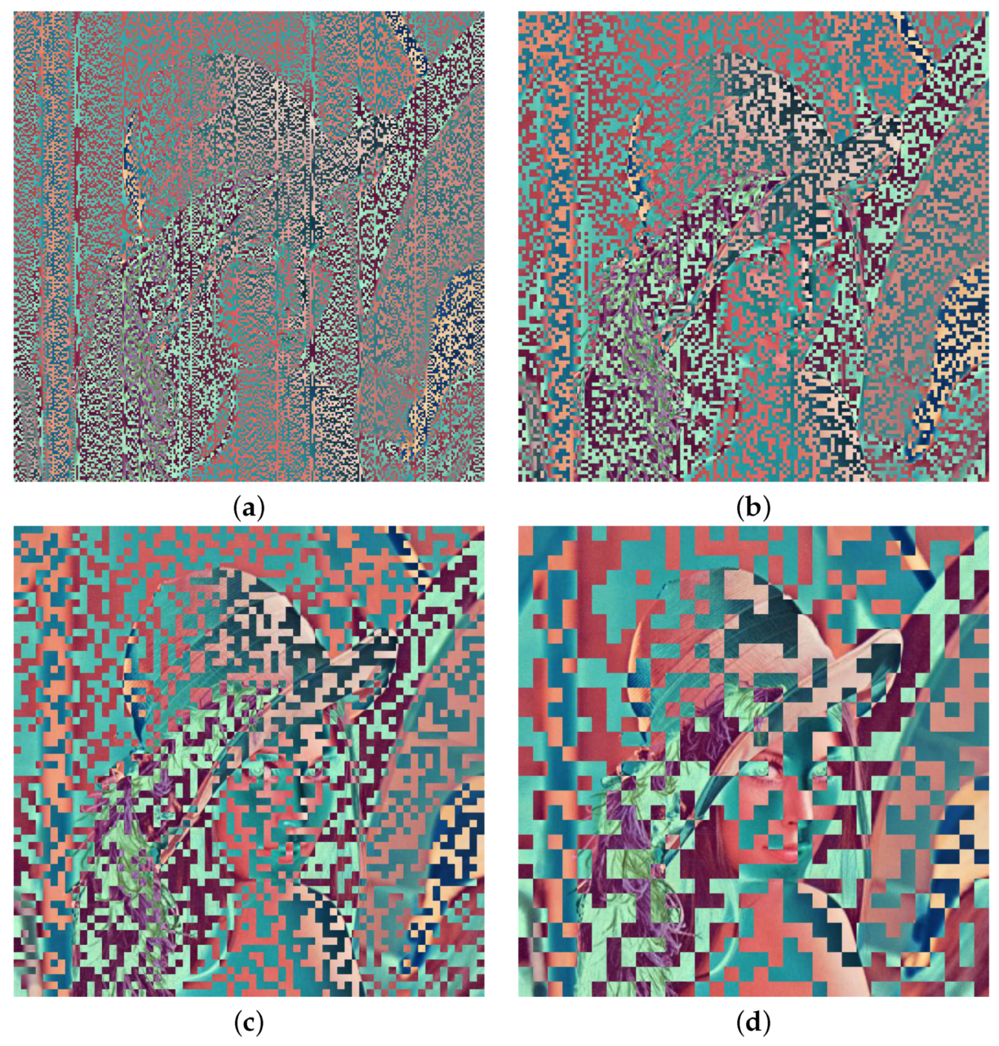
• The theorem of the symmetric histogram assumes that the NPT is independently applied. However, in larger pixel block sizes, particularly those of $8\times 8$ and greater, this independence is not rigorously maintained. The increased occurrence of pixels with the same intensity value in larger blocks may influence the independent application of the NPT. In such cases, multiple pixels sharing the same intensity level simultaneously are subject to the same single NPT application, resulting in a diminished symmetric appearance.
• The arithmetic mean of an encrypted pixel block using the NPT corresponds to the NPT of the original mean. Specifically, when $X=1$, the new value becomes the complement of 255, considering both the integer and decimal parts of the mean. Conversely, if $X=0$, the average remains unchanged.
• The variance, covariance, and correlation of a pixel block remain invariant under the NPT for any block size and magnitude measure. This was theoretically demonstrated and experimentally verified.
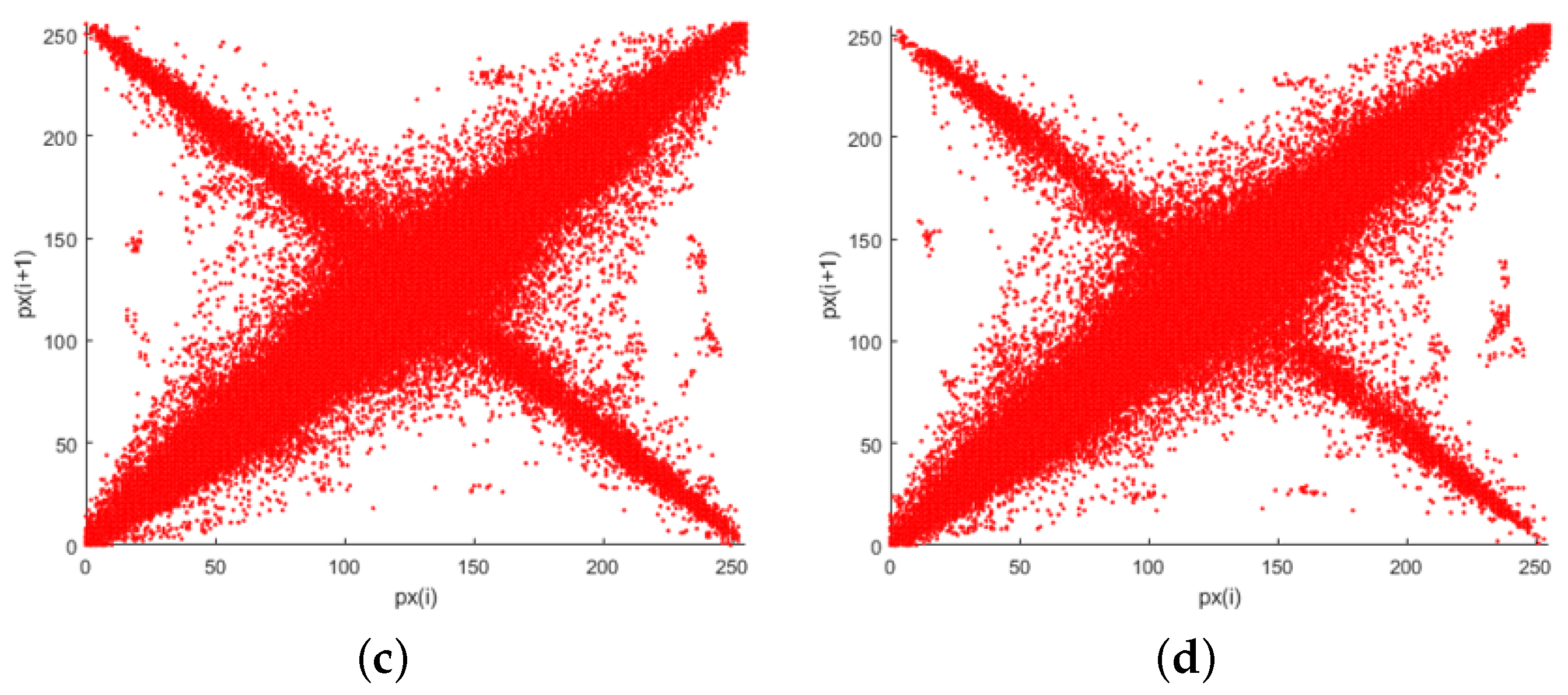
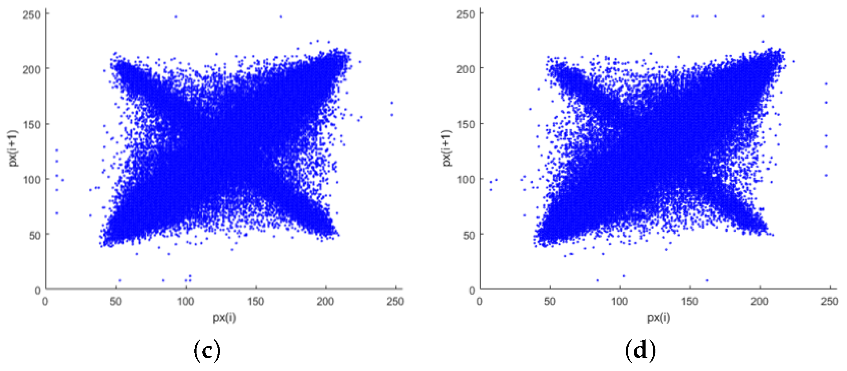
• Reflections are observed by plotting points of adjacent pixel values on a scatter plot after the NPT application. These reflections appear along one or two axes, specifically delimited by $x=127$ and $y=127$, with the origin point being $(127,127)$. The double reflection occurs when the NPT is applied with $X=1$ to both adjacent pixels. A single reflection occurs when the NPT operates with $X=1$ over only one of the two adjacent pixels, and they belong to different pixel blocks.
• Given that plain images exhibit a high linear correlation, the pairs of adjacent pixels are similar to a line $y=x$ on the scatter plot. After the NPT application, a graph in the form of “x” emerges on the scatter plot, resulting from vertical and/or horizontal reflections. Points on the line $y=-x$ indicate a single reflection, and this occurs only in pixel pairs from different blocks. As the number of blocks decreases (and the block size increases), the number of pixels over this line also decreases.
• The single application of NPT preserves the initial correlation within each pixel block, even though NPT can alter pixel values. As a technique for image encryption by pixel blocks, it proves insufficient for safeguarding data when there is initially high correlation. Additional encryption procedures must be applied afterward to modify pixel values and concurrently reduce correlation.
• Conversely, the NPT does not affect the efficacy of image compression algorithms such as JPEG, where a high correlation is desirable in pixel blocks. Therefore, this encryption technique can be incorporated into cryptosystems that are compatible with compression.

Limitations and Future Directions

Conducting a theoretical analysis of the individual security of an encryption technique encounters limitations in deriving results that can apply to any image. The study of these limitations allows for a more informed understanding of the technique’s applicability and the expected outcomes. The present work specifically examined the NPT within EtC systems, providing results on the histogram, mean, variance, covariance, and correlation that apply to any image, contrary to numerical analysis that reports results for specific images. However, it is crucial to acknowledge these limitations in future research works. Below, we describe some of them.

• Entropy. The conclusion regarding a symmetric histogram in the image after the NPT may prompt further research into other measures based on the histogram, such as entropy. However, this obtained result alone cannot provide a complete theoretical analysis of entropy after the NPT application. Since information entropy considers the probability, $p(I=h)$, that a pixel color value, I, has a specific intensity level h, this work has demonstrated that the frequencies of intensity level, h, are the same as the intensity level $l\oplus h$, and are equal to the average of these two. Therefore, the probability would tend to $p(I=h)=p(I=h\oplus 255)=(l_h+l_{h\oplus 255})/(2\times W\times H)$. Consequently, the Shannon entropy would transition from $E\left(I\right)=-{\sum }_{i=0}^{255}p(I=i){log}_{2}p(I=i)$ to approximately $E\left(I\right)=-2{\sum }_{i=0}^{127}p(I=i){log}_{2}p(I=i)$. This result does not offer clear information to conclude a reduction or increase in entropy.
• Image correlation. The correlation result obtained in this work applies to pixel blocks, as the NPT operates at the pixel block level. Extending this procedure to obtain the pixel correlation of the entire image presents a challenge. While the correlation of pixel blocks remains consistent before and after encryption, it does not necessarily imply this behavior for the correlation of the entire image. If pixel-block values change post-encryption, even with invariant individual correlations, the correlation of the entire image considers all the image pixels. The difficulty is located in the neighborhood pixels across different pixel blocks. Particularly, when a pixel block is encrypted with $X=1$ and an adjacent block with $X=0$, the correlation between pixel blocks may change, as their values do not necessarily change in the same direction. This dynamic interaction between pixel blocks makes it challenging to compute the theoretical correlation of the entire image.
• New encryption techniques. In the field of encryption schemes compatible with compression, there are two primary considerations: the security outcomes of the employed techniques and the impact of altering pixel values on compression performance. In the case of JPEG compression, it operates at the pixel block level. Preserving the correlation of the original image within pixel blocks is advantageous for its compression algorithm. This is why the NPT is employed for JPEG encryption, as it maintains pixel block correlations while altering the original values. However, it is noteworthy that the resulting distribution of pixel values does not approximate a uniform histogram. Producing new encryption techniques has the challenge of improving security and maintaining compression compatibility.

6. Conclusions

This paper presents a statistical analysis of encrypted images using the NPT technique, highlighting six theorems. These theorems were demonstrated and verified computationally to comprehend the security implications of applying the NPT. The resulting histogram of the image exhibits a symmetric shape because the expected frequencies of each pair of symmetric intensity levels are equal. Therefore, to achieve a uniform distribution, it is required that the sum of frequencies for each pair of symmetric intensities be the same. Additionally, horizontal and vertical reflections occur for couples of adjacent pixels on the scatter plot. Furthermore, the NPT preserves the initial correlation within each pixel block. This observation is significant, given that the primary objective of cryptography is to disassociate information. Consequently, it is imperative to incorporate operations, either before or after the NPT application, which reduces correlation, as the NPT itself does not alter it. However, this weakness makes it compatible with EtC algorithms, as they operate effectively when the correlation remains high. In conclusion, the NPT exhibits security vulnerabilities when employed for image encryption at the pixel block level. It is necessary to incorporate additional encryption techniques alongside the NPT that not only modify pixel values but also decrease correlation and generate uniform histograms. The challenge lies in ensuring that these techniques are also compatible with compression.

References

1. El Saj, R.; Sedgh Gooya, E.; Alfalou, A.; Khalil, M. Privacy-Preserving Deep Neural Network Methods: Computational and Perceptual Methods—An Overview. Electronics 2021, 10, 1367. [Google Scholar] [CrossRef]
2. Singh, K.N.; Singh, A.K. Towards integrating image encryption with compression: A survey. ACM Trans. Multimed. Comput. Commun. Appl. 2022, 18, 89. [Google Scholar] [CrossRef]
3. Aryal, A.; Imaizumi, S.; Horiuchi, T.; Kiya, H. Integrated algorithm for block-permutation-based encryption with reversible data hiding. In Proceedings of the 2017 Asia-Pacific Signal and Information Processing Association Annual Summit and Conference (APSIPA ASC), Kuala Lumpur, Malaysia, 12–15 December 2017; pp. 203–208. [Google Scholar] [CrossRef]
4. Imaizumi, S.; Kiya, H. A block-permutation-based encryption scheme with independent processing of RGB components. IEICE Trans. Inf. Syst. 2018, 101, 3150–3157. [Google Scholar] [CrossRef]
5. Aryal, A.; Imaizumi, S.; Horiuchi, T.; Kiya, H. Integrated Model of Image Protection Techniques. J. Imaging 2018, 4, 1. [Google Scholar] [CrossRef]
6. Imaizumi, S.; Ogasawara, T.; Kiya, H. Block-Permutation-Based Encryption Scheme with Enhanced Color Scrambling. In Proceedings of the Image Analysis: 20th Scandinavian Conference, SCIA 2017, Tromsø, Norway, 12–14 June 2017; Sharma, P., Bianchi, F.M., Eds.; Springer: Berlin/Heidelberg, Germany, 2017; pp. 562–573. [Google Scholar]
7. Motomura, R.; Imaizumi, S.; Kiya, H. Reversible Data Hiding in Compressible Encrypted Images with Capacity Enhancement. APSIPA Trans. Signal Inf. Proc. 2023, 12, e31. [Google Scholar] [CrossRef]
8. Sirichotedumrong, W.; Kinoshita, Y.; Kiya, H. Pixel-Based Image Encryption without Key Management for Privacy-Preserving Deep Neural Networks. IEEE Access 2019, 7, 177844–177855. [Google Scholar] [CrossRef]
9. Ahmad, I.; Shin, S. Perceptual Encryption-based Privacy-Preserving Deep Learning for Medical Image Analysis. In Proceedings of the 2023 International Conference on Information Networking (ICOIN), Bangkok, Thailand, 11–14 January 2023; pp. 224–229. [Google Scholar] [CrossRef]
10. Kenta, K.; Masanori, K.; Shoko, I.; Sayaka, S.; Hitoshi, K. An Encryption-then-Compression System for JPEG/Motion JPEG Standard. IEICE Trans. Fundam. Electron. Commun. Comput. Sci. 2015, E98.A, 2238–2245. [Google Scholar] [CrossRef]
11. Zhang, B.; Xiao, D.; Xiang, Y. Robust Coding of Encrypted Images via 2D Compressed Sensing. IEEE Trans. Multimed. 2021, 23, 2656–2671. [Google Scholar] [CrossRef]
12. Shimizu, K.; Suzuki, T.; Kameyama, K. Cube-Based Encryption-then-Compression System for Video Sequences. IEICE Trans. Fundam. Electron. Commun. Comput. Sci. 2018, E101.A, 1815–1822. [Google Scholar] [CrossRef]
13. Li, P.; Lo, K.T. Survey on JPEG compatible joint image compression and encryption algorithms. IET Signal Process. 2020, 14, 475–488. [Google Scholar] [CrossRef]
14. Maungmaung, A.; Kiya, H. A protection method of trained CNN model with a secret key from unauthorized access. APSIPA Trans. Signal Inf. Process. 2021, 10, e10. [Google Scholar] [CrossRef]
15. Ahmad, I.; Choi, W.; Shin, S. Comprehensive Analysis of Compressible Perceptual Encryption Methods–Compression and Encryption Perspectives. Sensors 2023, 23, 4057. [Google Scholar] [CrossRef] [PubMed]
16. Zhang, B.; Xiao, D.; Wang, M.; Liang, J. Privacy-Preserving Compressed Sensing for Image Simultaneous Compression-Encryption Applications. In Proceedings of the 2021 Data Compression Conference (DCC), Snowbird, UT, USA, 23–26 March 2021; pp. 283–292. [Google Scholar] [CrossRef]
17. Zhang, C.; Fan, H.; Zhang, M.; Lu, H.; Li, M.; Liu, Y. Plaintext-related image encryption scheme without additional plaintext based on 2DCS. Optik 2023, 272, 170312. [Google Scholar] [CrossRef]
18. SaberiKamarposhti, M.; Ghorbani, A.; Yadollahi, M. A comprehensive survey on image encryption: Taxonomy, challenges, and future directions. Chaos Solitons Fractals 2024, 178, 114361. [Google Scholar] [CrossRef]
19. Zhang, B.; Liu, L. Chaos-Based Image Encryption: Review, Application, and Challenges. Mathematics 2023, 11, 2585. [Google Scholar] [CrossRef]
20. Murillo-Escobar, M.A.; Meranza-Castillón, M.O.; López-Gutiérrez, R.M.; Cruz-Hernández, C. Suggested Integral Analysis for Chaos-Based Image Cryptosystems. Entropy 2019, 21, 815. [Google Scholar] [CrossRef]
21. Biban, G.; Chugh, R.; Panwar, A. Image encryption based on 8D hyperchaotic system using Fibonacci Q-Matrix. Chaos Solitons Fractals 2023, 170, 113396. [Google Scholar] [CrossRef]
22. Moya-Albor, E.; Romero-Arellano, A.; Brieva, J.; Gomez-Coronel, S.L. Color Image Encryption Algorithm Based on a Chaotic Model Using the Modular Discrete Derivative and Langton’s Ant. Mathematics 2023, 11, 2396. [Google Scholar] [CrossRef]
23. Sun, J.; Ma, Y.; Wang, Z.; Wang, Y. Dynamic analysis and cryptographic application of a 5D hyperbolic memristor-coupled neuron. Nonlinear Dyn. 2023, 111, 8751–8769. [Google Scholar] [CrossRef]
24. Lai, Q.; Zhang, H. A new image encryption method based on memristive hyperchaos. Opt. Laser Technol. 2023, 166, 109626. [Google Scholar] [CrossRef]
25. Lidong, L.; Jiang, D.; Wang, X.; Zhang, L.; Rong, X. A Dynamic Triple-Image Encryption Scheme Based on Chaos, S-Box and Image Compressing. IEEE Access 2020, 8, 210382–210399. [Google Scholar] [CrossRef]
26. Kiya, H.; Maung, A.P.M.; Kinoshita, Y.; Imaizumi, S.; Shiota, S. An overview of compressible and learnable image transformation with secret key and its applications. APSIPA Trans. Signal Inf. Proc. 2022, 11, e11. [Google Scholar] [CrossRef]
27. Puchala, D.; Stokfiszewski, K.; Yatsymirskyy, M. Image Statistics Preserving Encrypt-then-Compress Scheme Dedicated for JPEG Compression Standard. Entropy 2021, 23, 421. [Google Scholar] [CrossRef]
28. Ahmad, I.; Shin, S. A Perceptual Encryption-Based Image Communication System for Deep Learning-Based Tuberculosis Diagnosis Using Healthcare Cloud Services. Electronics 2022, 11, 2514. [Google Scholar] [CrossRef]
29. Chuman, T.; Kurihara, K.; Kiya, H. On the security of block scrambling-based ETC systems against jigsaw puzzle solver attacks. In Proceedings of the 2017 IEEE International Conference on Acoustics, Speech and Signal Processing (ICASSP), New Orleans, LA, USA, 5–9 March 2017; pp. 2157–2161. [Google Scholar] [CrossRef]
30. Chuman, T.; Kurihara, K.; Kiya, H. Security evaluation for block scrambling-based ETC systems against extended jigsaw puzzle solver attacks. In Proceedings of the 2017 IEEE International Conference on Multimedia and Expo (ICME), Hong Kong, China, 10–14 July 2017; pp. 229–234. [Google Scholar] [CrossRef]
31. Iida, K.; Kiya, H. Privacy-Preserving Content-Based Image Retrieval Using Compressible Encrypted Images. IEEE Access 2020, 8, 200038–200050. [Google Scholar] [CrossRef]
32. Chuman, T.; Sirichotedumrong, W.; Kiya, H. Encryption-Then-Compression Systems Using Grayscale-Based Image Encryption for JPEG Images. IEEE Trans. Inf. Forensic Secur. 2019, 14, 1515–1525. [Google Scholar] [CrossRef]
33. Sirichotedumrong, W.; Kiya, H. Grayscale-based block scrambling image encryption using ycbcr color space for encryption-then-compression systems. APSIPA Trans. Signal Inf. Process. 2019, 8, e7. [Google Scholar] [CrossRef]
34. Hosny, K.M.; Zaki, M.A.; Lashin, N.A.; Fouda, M.M.; Hamza, H.M. Multimedia Security Using Encryption: A Survey. IEEE Access 2023, 11, 63027–63056. [Google Scholar] [CrossRef]
35. Kumar, A.; Dua, M. A GRU and chaos-based novel image encryption approach for transport images. Multimed. Tools Appl. 2023, 82, 18381–18408. [Google Scholar] [CrossRef]
36. Mamia, S.B.; Puteaux, P.; Puech, W.; Bouallegue, K. From Diffusion to Confusion of RGB Pixels Using a New Chaotic System for Color Image Encryption. IEEE Access 2023, 11, 49350–49366. [Google Scholar] [CrossRef]
37. Wroughton, J.; Cole, T. Distinguishing between binomial, hypergeometric and negative binomial distributions. J. Stat. Educ. 2013, 21, 1. [Google Scholar] [CrossRef]
38. Seong, J.H.; Seo, D.H. Wi-Fi fingerprint using radio map model based on MDLP and euclidean distance based on the Chi squared test. Wirel. Netw. 2019, 25, 3019–3027. [Google Scholar] [CrossRef]
39. Sei, Y.; Ohsuga, A. Privacy-preserving chi-squared test of independence for small samples. BioData Min. 2021, 14, 6. [Google Scholar] [CrossRef]
40. Musanna, F.; Dangwal, D.; Kumar, S. Novel image encryption algorithm using fractional chaos and cellular neural network. J. Ambient. Intell. Humaniz. Comput. 2022, 8, 2205–2226. [Google Scholar] [CrossRef]
41. Burger, W.; Burge, M.J. Histograms and Image Statistics. In Digital Image Processing: An Algorithmic Introduction, 3rd ed.; Springer International Publishing: Cham, Switzerland, 2022; pp. 29–48. [Google Scholar] [CrossRef]
42. Kammoo, P.; Neammanee, K.; Laipaporn, K. The local limit theorem for general weighted sums of Bernoulli random variables. Commun. Stat. Theory Methods 2023, 0, 1–9. [Google Scholar] [CrossRef]
43. Evans, M.J.; Rosenthal, J.S. Probability and Statistics: The Science of Uncertainty, 2nd ed.; W.H. Freeman: New York, NY, USA, 2009; pp. 159–166. [Google Scholar]
Figure 1. The negative–positive transformation (NPT) as a component of the EtC system for image encryption [33].
Mathematics 12 00908 g001
Figure 2. Possible reflections of a pixel value pair ( r , s ) after NPT. (a) Original position. (b) Vertical reflection across the abscissa axis. (c) Reflection over both axes. (d) Horizontal reflection across the ordinate axis.
Mathematics 12 00908 g002
Figure 3. The Lena image, measuring 512 × 512 pixels, is utilized in this section for encryption, using the NPT to validate the presented theorems.
Mathematics 12 00908 g003
Figure 4. Lena’s original histograms and scatter plots. (a) Histogram of the red channel. (b) Histogram of the green channel. (c) Histogram of the blue channel. (d) Scatter plot of the red channel. (e) Scatter plot of the green channel. (f) Scatter plot of the blue channel.
Mathematics 12 00908 g004
Figure 5. Encryption results of the Lena image using the NPT for various block sizes. (a) Pixel block size of 2 × 2 . (b) Pixel block size of 4 × 4 . (c) Pixel block size of 8 × 8 . (d) Pixel block size of 16 × 16 .
Mathematics 12 00908 g005
Figure 6. Resultant histograms of the red channel from Figure 5. (a) Red channel histogram from Figure 5a. (b) Red channel histogram from Figure 5b. (c) Red channel histogram from Figure 5c. (d) Red channel histogram from Figure 5d.
Mathematics 12 00908 g006
Figure 7. Resultant histograms of the green channel from Figure 5. (a) Green channel histogram from Figure 5a. (b) Green channel histogram from Figure 5b. (c) Green channel histogram from Figure 5c. (d) Green channel histogram from Figure 5d.
Mathematics 12 00908 g007aMathematics 12 00908 g007b
Figure 8. Resultant histograms of the blue channel from Figure 5. (a) Blue channel histogram from Figure 5a. (b) Blue channel histogram from Figure 5b. (c) Blue channel histogram from Figure 5c. (d) Blue channel histogram from Figure 5d.
Mathematics 12 00908 g008
Figure 9. Resultant scatter plots of the red channel from Figure 5. (a) Red channel scatter plot from Figure 5a. (b) Red channel scatter plot from Figure 5b. (c) Red channel scatter plot from Figure 5c. (d) Red channel scatter plot from Figure 5d.
Mathematics 12 00908 g009aMathematics 12 00908 g009b
Figure 10. Resultant scatter plots of the green channel from Figure 5. (a) Green channel scatter plot from Figure 5a. (b) Green channel scatter plot from Figure 5b. (c) Green channel scatter plot from Figure 5c. (d) Green channel scatter plot from Figure 5d.
Mathematics 12 00908 g010
Figure 11. Resultant scatter plots of the blue channel from Figure 5. (a) Blue channel scatter plot from Figure 5a. (b) Blue channel scatter plot from Figure 5b. (c) Blue channel scatter plot from Figure 5c. (d) Blue channel scatter plot from Figure 5d.
Mathematics 12 00908 g011aMathematics 12 00908 g011b