Abstract
Many practical problems can be classified as constrained multi-objective optimization problems. Although various methods have been proposed for solving constrained multi-objective optimization problems, there is still a lack of research considering the integration of multiple constraint handling techniques. Given this, this paper combines the objective and constraint separation method with the multi-operator method, proposing a population feasibility state guided autonomous constrained evolutionary optimization method. This method first defines the feasibility state of the population based on both feasibility and feasibility of the solutions. Subsequently, a reinforcement learning model is employed to construct a mapping model between the population state and reproduction operators. Finally, based on the real-time population state, the mapping model is utilized to recommend the promising reproduction operator for the next generation. This approach demonstrates significant performance improvement for constrained mechanisms in constrained multi-objective optimization algorithms, and shows considerable advantages in comparison with state-of-the-art constrained multi-objective optimization algorithms.
Keywords:
constrained multi-objective optimization problems; population feasibility state; autonomy; evolutionary optimization; reinforcement learning MSC:
49M41
1. Introduction
Constrained multi-objective optimization problems (CMOPs) refer to optimizing multiple conflicting performance metrics simultaneously while ensuring that decision variables meet the constraints of the objective problem. Many real-world problems can be classified as CMOPs, such as integrated energy dispatch [1], multi-stage portfolio [2], and spacecraft orbit optimization [3]. Without loss of generality, a CMOP can be defined as
where represents the decision variables, is the -th objective function for . represents the -th inequality constraint for . represents the -th equality constraint for . and are lower and upper boundaries of , respectively, and generates a random number between and . The wide application in real-world problems makes the performance testing of the constrained multi-objective optimization algorithm more demanding; therefore, many real-world test suites, such as RC [4], have been proposed in the existing research, and the challenges of solving constrained multi-objective optimization problems can be studied in depth.
While meeting the problem constraints, the decision variables in CMOPs also need to be optimized for improving multiple conflicting objective functions simultaneously. This difficulty contributes to the challenging nature of solving multi-objective optimization problems. The key to solving CMOPs lies in constraint handling. Applying appropriate constraint handling methods ensures a balance between the feasibility of solutions, convergence, and diversity in the objective space. Currently, common constraint handling methods include the penalty function method, the objective and constraint separation method, the multi-objective method, the transformation method, the mixed method, and the multiple-operator method [5]. In the objective and constraint separation method, the constraint method is an effective constraint handling approach, which is capable of leveraging information from relatively good infeasible solutions to guide the evolution of the population to some extent. However, the constraint method also has limitations. For example, the setting of values often relies on human experience, which can lead to biases in the population search direction. It is, therefore, important to adjust the search direction for the constraint method. To adjust the search direction, the multiple-operator method is a candidate. In this method, use of different reproduction operators leads to the generation of diverse types of solutions, aiding in adjusting the search direction of the population [3,6,7,8]. However, the selection of reproduction operators also usually relies on subjective human experience, making it tough to determine the timing and scope of their application. Therefore, combining the constraint method with the multi-operator method poses a challenge.
In light of this, this paper combines the objective and constraint separation method with the multi-operator method, proposing a population feasibility state guided autonomous constrained evolutionary optimization method. This method first establishes the population state based on both feasibility and feasibility of the solutions. Subsequently, a reinforcement learning model is employed to construct a mapping model between the population state and the operator. Finally, based on the real-time population state, the mapping model is utilized to recommend the subsequent reproduction operator for the next generation.
The main contributions of this paper are summarized as follows:
- (1)
- Proposing a self-guided optimization method that combines the objective and constraint separation method with the multi-operator method. Specifically, this method combines the constraint method with the multi-operator method, using the multi-operator approach to enhance the diversity of solutions with more search directions. Adjusting the population search direction helps reduce the dependence of the constraint method on human experience for setting values. Additionally, overcoming the limitations of the multi-operator method relying on human experience using reinforcement learning further enhances the algorithm’s performance. This holds potential to contribute to the field of combining various constraint handling methods.
- (2)
- Proposing a novel method for characterizing the population state. Existing research has not characterized the population state from the perspective of both feasibility and feasibility of population solutions, limiting the perception of the population’s feasibility state. The proposed method for characterizing population state in this paper contributes to the description of population state in the field of autonomous intelligent optimization.
The rest of this paper is organized as follows. Section 2 reviews the relevant research works and points out the existing problems in the current research. The proposed method is described in Section 3, including the characterization of the population state, the population’s reproduction operators, and their performance evaluation. Section 4 is the experimental results and analysis. Finally, Section 5 summarizes the whole paper and discusses future research directions.
2. Related Works
This paper proposes a solving approach for constrained multi-objective optimization problems by combining the objective and constraint separation method with the multi-operator method. Hence, this section primarily reviews existing methods for constraint handling. Given that our method focuses on the objective and constraint separation method, as well as the multi-operator method, a review of the progress of research on these two approaches is also provided.
2.1. Constrained Multi-Objective Evolutionary Optimization
Constraint handling is a crucial task in addressing constrained multi-objective problems. The penalty function method is a common approach for constraint handling. The idea is to construct a penalty term based on the degree of constraint violation and incorporate this penalty term into the objective function. This transforms the constrained optimization problem into an unconstrained optimization problem. The setting of the penalty factor has a significant impact on the algorithm. Setting the penalty factor to be too large or too small both have negative effects. If the feasible region consists of several disconnected and independent subregions, setting the penalty factor too large may lead to premature convergence of the population and narrow down the located search space. On the other hand, setting the penalty factor too small may render the constraint conditions ineffective, making it challenging for the population to converge. In light of this, existing research has considered the use of variable penalty factors. In the method proposed by Jiao et al. [9], the penalty factor is dynamically adjusted based on the ratio of feasible solutions in a real-time population. In the dynamic penalty function method proposed by Maldonado et al. [10], the penalty factor undergoes gradual adjustments with changes in the population generations. Furthermore, in the learning-guided parameter tuning method proposed by Fan et al. [11] an adaptively generated penalty factor significantly enhances the adaptability of the penalty factor. From this, it is evident that the penalty function method is straightforward, yet the proper setting of the penalty factor is still challenging and usually relies on human expertise.
The hybrid method bridges evolutionary algorithms with traditional optimization methods, effectively integrating the strengths of evolutionary algorithms and mathematical programming. This approach aims to maintain both population convergence and diversity, while emphasizing the feasibility of optimized solutions. In general, evolutionary algorithms guide the population towards promising regions, and mathematical programming further explores feasible solutions within the located region. Morovati et al. [12] combined evolutionary algorithms with the Zoutendijk feasible direction method to search for solutions that meet both optimization objectives and constraints. Schutze et al. [13] utilize traditional optimization methods to explore information about nearby solutions of population. They predict the subsequent evolutionary direction of the population, guiding it towards the feasible regions. The hybrid approach is a comprehensive method that combines global and local search capabilities, effectively balancing optimization objectives and constraint satisfaction. However, the timing of integrating evolutionary algorithms and mathematical programming still requires further research.
The idea behind multi-objective optimization is to transform constrained multi-objective optimization problems into unconstrained multi-objective optimization problems. In contrast to the penalty function method, this approach transforms constraints into one or more optimization objectives. Through continuous population evolution, the method optimizes the transformed objectives, aiming to reduce the degree of constraint violation. Various methods may transform constraint conditions into a different number of optimization objectives. Long et al. [14] converted all constraints into a single optimization objective related to the degree of constraint violation. Vieira et al. [15]. transformed constraint conditions into two optimization objectives: the total degree of constraint violation and the number of violated constraints. Ming et al. [16] transformed constraint conditions into three optimization objectives. Compared with the penalty function method, this method offers greater flexibility in handling constraint conditions. However, as the number of transformed objective functions increases, the handling complexity also rises.
2.2. The Objective and Constraint Separation Method
The idea behind the objective–constraint separation method is to handle the problem’s objective and constraints separately. While reducing the degree of constraint violation, it also optimizes the objective functions. The conventional methods include the constrained dominance principle (CDP) [17], the constrained method [18], and stochastic ranking (SR) [19].
2.2.1. Constraint Dominance Principle
In the CDP, for solutions and , is considered to be non-dominated to when any of the following conditions is satisfied:
- (1)
- Both and are feasible solutions, but has a better optimization objective value.
- (2)
- is a feasible solution, whereas is an infeasible solution.
- (3)
- Both and are infeasible solutions, but , where represents the degree of constraint violation for the optimization solution.
The selection principle of CDP is relatively straightforward, as it tends to retain feasible solutions and eliminate infeasible ones, leading the population to be prone to local optima.
Deb et al. [17] proposed the abovementioned constraint handling method, which to some extent alleviates the solving pressure associated with constrained multi-objective problems. Subsequently, to utilize effective information from infeasible solutions, Saha and Ray [20] introduced a probability point-based method for repairing equality constraints.
2.2.2. ε Constrained Method
In the constraint method, the approach involves relaxing constraints and gradually reducing the value of to tighten the constraints. This method utilizes information from excellent infeasible solutions to guide the population towards the feasible region during evolution. When , the constraint method is equivalent to CDP. For solutions and , is considered to be non-dominated to when either of the following conditions is satisfied:
- (1)
- Both and are feasible solutions, but has a better optimization objective value.
- (2)
- is an feasible solution, whereas is not an feasible solution.
- (3)
- Both and are not feasible solutions, but , where represents the degree of constraint violation for the optimization solution.
The constraint method to some extent utilizes information from excellent infeasible solutions, but the choice of often relies on human expertise, which may still lead the population into local optima. Sana Ben Hamida et al. [21] tried to propose an -based algorithm by temporarily tolerating high violation degrees to expand the feasible region, and gradually narrowing the feasible region to enhance global search capability. This method effectively utilizes information from infeasible solutions, thereby guiding the population moves from infeasible regions to feasible regions, improving the algorithm’s performance. In addition, the small habitat technique with an adaptive radius can be used to extend the penalty function. Ponsich et al. [22] incorporated constraint violation and a scalar function as optimization objectives, transforming CMOPs into bi-objective problems. They integrated the constraint method into MOEA/D to prove the performance on solving the CMOPs.
2.2.3. Stochastic Ranking
SR refers to the probabilistic selection of constraint dominance and objective dominance to better generate offspring populations. Compared with the two methods mentioned above, this approach better utilizes valuable information from excellent infeasible solutions, increases the diversity of the population, avoids premature convergence of the population, and enhances global search capability. However, the setting of selection probabilities still relies on human expertise, which may lead to the population falling into local optima. SR has diverse applications, each of which possesses flexible performance and functionality. Liu et al. [23] combined indicator-based MOEA with CDP, the constraint method, and the SR method, respectively. They proposed multiple indicator-based constrained multi-objective methods, separately studying their solution performance. Jan and Khanum [24] first embedded SR in the framework of the decomposition-based multi-objective evolutionary algorithm (MOEA/D), effectively enhancing the algorithm’s performance. Ying et al. [25] drew inspiration from simulated annealing and proposed an annealing SR mechanism. This mechanism can fully utilize well-behaved feasible solutions, guiding the evolution toward global optima. Sabat et al. [26] combined particle swarm optimization with SR, proposing a new hybrid algorithm for solving standard-constrained engineering design problems. The proposed hybrid algorithm leverages the domain independence of SR and the faster convergence of particle swarm optimization. To address the drawback of setting SR parameters relying on manual expertise, some scholars have proposed methods for adaptively adjusting SR parameters. Li et al. [27] adaptively randomize sorting based on the dynamic balance of convergence and diversity in the population’s state in high-dimensional space. Ying et al. [28] proposed an adaptive SR mechanism by dynamically controlling probability parameters based on the difference between the current evolutionary stage and the degree of individual constraint violation. Gu et al. [29] proposed an enhanced SR strategy correlating fitness and probability operators, which comprehensively considers the convergence and diversity of the population to improve the quality of candidate solutions. There are various methods for adjusting evaluation indicators using SR, each with its characteristics. Wang et al. [30] introduced a logistic regression model to correct surrogate-assisted fitness evaluations and employed SR to further reduce the impact of the approximate constraint function. Li et al. [31] proposed a multi-objective algorithm for multi-objective optimization problems, which utilized SR techniques to balance search biases across different objectives. Chen et al. [32] proposed a multi-objective algorithm based on gradient SR. This employed a two-layer gradient SR method for offspring selection, guiding the direction of Pareto front selection and enhancing the relationships between different indicators in indicator-based MOEA.
2.3. The Multi-Operator Method
The dynamic selection of multiple reproduction operators can influence the distribution of the population in the search space. The fundamental idea of the multi-operator method is that of performing different reproduction operators on population to meet the solving requirements. The selected multiple reproduction operators need to balance well the feasibility, convergence, and diversity of the solution set. In the multi-operator algorithm proposed by Yu et al. [33], infeasible solutions are reproduced with special mutation operators from the mutation operator pool with a certain probability. In the approach proposed by Xu et al. [34], distinct mutation strategies are applied to feasible and infeasible solutions, facilitating the population’s rapid evolution toward the feasible region. Liu et al. [35] divided the entire population into multiple subpopulations, with each subpopulation adopting different crossover operators. This approach facilitates the population in escaping local optima and fully exploring the search space. He et al. [36] implemented different crossover and mutation operators for feasible solutions and good infeasible solutions, driving the infeasible solutions toward the feasible region. Tian et al. [37] employed deep reinforcement learning to select different operators at different stages, striking a balance between the diversity and convergence of the population. Zuo et al. [38] also used deep reinforcement learning to dynamically employ reproduction operators, which can be embedded into existing evolutionary algorithms and improve their performance.
It can be observed that the multi-operator method can adapt to the solving requirements, balancing the feasibility, convergence, and diversity of optimized solutions. However, because the multi-operator method usually relies on manual expertise, configuring performance-complementary reproduction operators, and determining the appropriate timing or scope of using reproduction operator poses a challenge.
2.4. Discussion
From this section, it can be inferred that the objective and constraint separation method is simple to conduct; however, using a single reproduction operator may lead to a biased search direction for the population. Therefore, it is necessary to employ multiple reproduction operators to adjust the population’s search directions. The multi-operator method can enhance the population diversity but this often relies on human expertise to determine the timing and scope of using different operators. Similar to the difficulty in using the constraint separation method, reliance on human expertise is one of the limitations of the multi-operator method, and this results in a subjective determination of the timing and scope for the use of different operators. Using reinforcement learning methods can effectively reduce the dependence on human expertise. This indicates that combining reinforcement learning with the objective and constraint separation method, and the multi-operator method can leverage strengths and mitigate weaknesses, which has promising prospects for improving algorithm performance.
In light of this, a self-evolving optimization approach guided by the feasibility state of the population is proposed in Section 3, which leverages the feasibility state of population solutions within a reinforcement learning framework to recommend the reproduction operator choices for population evolution. This significantly enhances the autonomy of solving problems, avoiding the subjectivity caused by human expertise.
3. The Proposed Method
3.1. Overall Framework
This section introduces the population feasibility state guided autonomous evolutionary optimization method. It first characterizes the feasibility state of the population solutions based on both feasibility and feasibility of the solutions, where the individual of population is presented as . Subsequently, a real-time mapping model between the state of solutions and reproduction operator choices based on the Q-learning reinforcement learning model is constructed. Finally, based on the current state of the population, the mapping model is utilized to recommend the reproduction operator to generate offspring population. This method exhibits a significant performance improvement for constrained multi-objective optimization algorithms employing the constraint mechanism. By employing the aforementioned method, it becomes possible to autonomously select appropriate reproduction operators for different population states, efficiently addressing constrained multi-objective optimization problems. Q-learning is used to build the mapping relationship between population state and operators. The reason for using Q-learning is that we regard dynamically selecting operators for varying populations as a Markov decision process, and Q-learning is an excellent reinforcement learning algorithm used to solve Markov decision process problems. The ability of Q-learning includes the following aspects:
- (1)
- Learning the optimal strategy: Q-learning can learn the optimal strategy, that is, taking actions that can maximize cumulative returns in each state. By continuously updating the Q-value table, the agent can gradually converge to the optimal strategy.
- (2)
- No model required: Q-learning does not require modeling of the environment; that is, it does not require prior knowledge of state transition probabilities and reward functions. It learns the Q-value function through interaction with the environment, thus achieving model free learning.
- (3)
- Adaptability: Q-learning can adapt to different environments and tasks. It can handle continuous state space and action space.
- (4)
- Convergence: Under certain conditions, the Q-learning algorithm can converge to the optimal Q-value function. This means that the agent can learn the optimal strategy within a limited time.
An analogy for the concept of evolutionary computation is that of reinforcement learning. Population is analogous to agent, population state is analogous to agent state, operator is analogous to action, indicator-based population evaluation is analogous to reward, and fitness landscape is analogous to environment.
The overall framework of the proposed method is illustrated in Algorithm 1. Regarding existing constrained multi-objective optimization algorithms, the method proposed in this paper only requires the incorporation of two steps in the algorithm process. One is the selection of the reproduction operator; the other is Q-value learning. Specifically, begin by initializing the relevant parameters for reinforcement learning, along with the Q-table for storing Q-values and the Count-table for tracking the frequency of action selections. Then, in each generation, select the reproduction operator according to Algorithm 2 to generate offspring populations. Finally, update the Q-value table with according to Algorithm 3. The whole flowchart of the proposed method is presented in Figure 1, where the extra modules required by this method are highlighted.
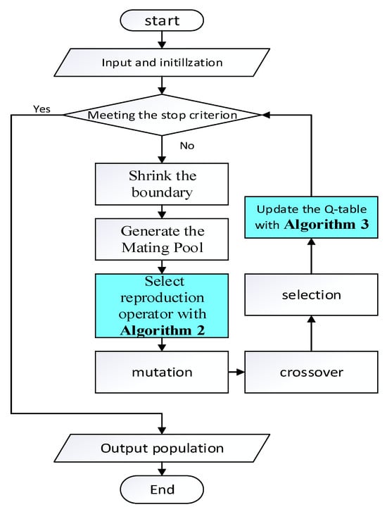
Figure 1.
A flowchart of the overall framework.
The methods for selecting the reproduction operator and updating the Q-value table are outlined in Sections B and C, respectively.
| Algorithm 1 Overall framework |
| Input: Maximum generation , Population size , Problem dimension , Scaling factor in DE operator , Crossover reward update parameter , reward predictability parameter , greedy strategy parameter . Output |
| 1. ; |
| 2. with equation (4) |
| 3. ; |
| 4. ; |
| 5. 0.005, 0.2, 0.8; |
| 6. 0 0; |
| 7. , ; |
| 8. ; |
| 9. do |
| 10. ; |
| 11. Select operator with Algorithm 2; |
| 12. ; |
| 13. ; |
| 14. For = 1: |
| 15. ; |
| 16. ; |
| 17. ; |
| 18. ; |
| 19. end |
| 20. ; |
| 21. ; |
| 22. with Algorithm 3 to update Q-table; |
| 23. ; |
| 24. , ; |
| 25. ; |
| 26. End while |
| 27. ; |
3.2. The Selection of Reproduction Operator
3.2.1. Reproduction Operator for Regulating Population State
In evolutionary algorithms, regulating the population state is achieved through different reproduction operators, each with its advantages and disadvantages. Therefore, employing different reproduction operators for different population states has a significant impact on population regulation. Among various evolutionary algorithms, Differential Evolution (DE) [38] and Genetic Algorithm (GA) [9] are very typical and have been widely applied. The reproduction operator in DE typically exhibits good convergence, while the reproduction operator in GA possesses strong global search capabilities. Combining the reproduction operator of DE and GA enables a balance between global exploration and local exploitation, contributing to the improvement of the algorithm’s search performance. Therefore, this paper considers using two reproduction operators from DE and GA to generate high-quality offspring populations.
| Algorithm 2 Two-stage reproduction operator selection |
| Input: current generation , Q-table, Count-table; ; |
| 1. then |
| 2. ; |
| 3. Else |
| 4. ; |
| 5. }; |
| 6. End if |
| 7. then |
| 8. ; |
| 9. End if |
With this approach, there are two reproduction operators used for regulating the population state. Let us denote as the identifier of the reproduction operator adopted by population . The possible values and their meanings are as follows: represents the execution of the reproduction operator from DE, and represents the execution of the reproduction operator from GA.
3.2.2. Two-Stage Reproduction Operator Selection
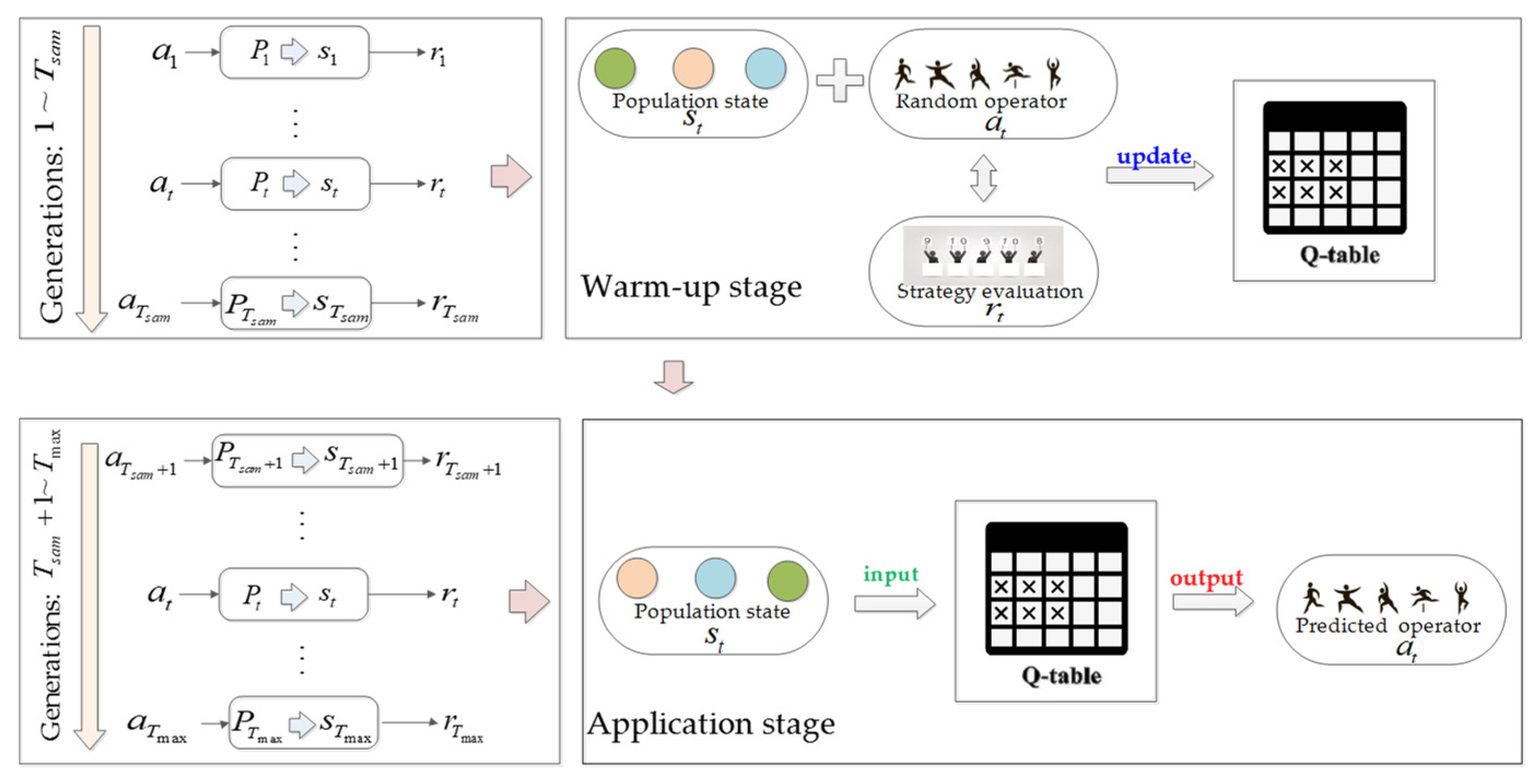
In the early stage of the evolutionary search, due to the unavailability of sufficient training samples, the Q-value table (Q-table) cannot provide effective guidance on reproduction operator choices. Therefore, the evolution of the population is divided into two stages. First, from the generation to the generation, it is the reinforcement learning warm-up stage, where samples are collected for updating the Q-table. Second, from the generation until the end of the population evolution, it is the application stage of reinforcement learning. This two-state operator selection assisted by Q-learning can be visualized in Figure 2, and its implementation details are illustrated in Algorithm 2. In Algorithm 2, the first stage involves randomly selecting the reproduction operator to accumulate training samples and update the Q-table. In the application stage, for the evolutionary population at generation , the state of this population is used as input to the Q-table to obtain performance predictions for different reproduction operators. Denote the performance prediction obtained after applying the reproduction operator to as . For all reproduction operators, let
denote the reproduction operator with the maximum performance prediction. So, is the reproduction operator adopted for the subsequent evolution of the population.
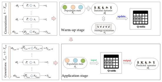
Figure 2.
The embedded evolutionary algorithm and Q-learning.
It is worth noting that the frequency of choosing each reproduction operator has a significant impact on the Q-table updates and may result in inaccurate predicted Q-values. Therefore, this paper also records the frequency of reproduction operator choices in the Count-table to calculate the average Q-value for each population state , aiming to improve the accuracy of Q-value predictions and ensure the stability of algorithm performance. Hence, the abovementioned is obtained by
To mitigate the negative impact of overfitting in Q-learning and enhance the exploration capability of the population state space, this paper borrows the Epsilon–Greedy strategy. With a small probability , a strategy is randomly chosen from the reproduction operator space instead of the one recommended by the Q-table. This operator is then used for the subsequent evolution of the population. The based operator selection is presented by
where means a random operator is selected.
3.3. Update the Q-Table
The updating of the Q-table is illustrated in Algorithm 3. Firstly, calculate the proportion of feasible and feasible solutions in the population to obtain . Then, calculate by comparing and . Finally, update the Q-value table based on the adopted and record the update frequency in the corresponding position of the Count-table.
3.3.1. Characterizing the Population State Based on the Feasibility of Population
In constrained multi-objective evolutionary algorithms (CMOEAs), a representing decision variables is regarded as a population individual, and the -th population individual is denoted as . Hence, a population with individuals in the -th generation is denoted as , where . is initialized by
and are lower and upper boundaries, respectively. During the evolution of , its feasibility and -feasibility are two important pieces of knowledge during the population evolution process. Both of them influence the search direction and efficiency of the algorithm. In view of this, the proportions of both can be used to jointly characterize the population state. As introduced in DCNSGA-II, the normalized average degree of the constraint violation of on all constraints is regarded as the constraint violation objective by
where , , and are the dynamic constraint boundaries, , is the maximum number of generations. and are updated following the same criterion. As an example, is updated by
where is a close-to-zero value ( = 1 × 10⁻⁸) and controls the decreasing trend of . and are updated as follows:
With , the constraint violation degree is computed. Thus, the population state can be characterized. Firstly, calculate the proportions of feasibility
and -feasibility in the population by
where is the population size, and are number of feasible population and -feasible population. Next, divide the proportions of both in the population into three parts, respectively, including zero to one-third, one-third to two-thirds, and two-thirds to one. Consider that feasibility proportion is not higher than the -feasibility proportion, so the population only contains six states, denoted as
| Algorithm 3 Update the Q-table |
| Input parameters of Q-learning, Count-table, Q-table; |
| Output: Q-table, Count-table; |
| 1. ; |
| 2. then |
| 3. ; |
| 4. Else |
| 5. ; |
| 6. End if |
| 7. ; |
| 8. Count-tableCount-table(; |
3.3.2. Stage-Wise Evaluation of Population Solutions
This paper adopts a stage-wise evaluation method. If the evolved population has no feasible solutions, the performance of reproduction operators is evaluated based on the extent to which the constraint violation of the best individual in the population increases or decreases. Considering the best individual in population , apply the strategy of this population as . To evaluate the performance of , calculate the violation degree of this individual for each constraint, summing up these violation degrees to obtain the overall constraint violation degree . Then, the performance of the reproduction operator , denoted as , can be expressed as
It can be observed that the values of fall within the range of 0 to 1. It is worth noting that means applying the reproduction operator does not lead to an improvement in the population’s satisfaction with constraints. means applying , the best individual in the population becomes a feasible solution.
When the evolved population contains one or more feasible solutions to the problem, the performance of reproduction operators is evaluated based on the extent to which the Hypervolume (HV) indicator of feasible solutions improves. The Hypervolume (HV) not only reflects the diversity of feasible solutions but also indicates the convergence of these solutions. For the population , calculate the HV indicator of feasible solutions in this population, denoted as . Then, the performance of reproduction operator can be expressed as
measures the volume of the objective space enclosed by the obtained solution set in and a reference point , which can be obtained by
where represents the Lebesgue measure. With this approach, the performance of the reproduction operator can be expressed as
3.3.3. Q-Value Update
This paper employs the Q-value function for updating the Q-value table, and its functional expression is as follows:
where is the learning rate controlling the willingness to accept newly observed information. is the immediate reward obtained after taking action . is the discount factor, indicating the importance given to future rewards. is the next state transitioned to after taking action . represents the Q-value corresponding to choosing the optimal action in the next state . By constantly interacting with the population evaluation function, the population can choose an operator based on the current state and update the corresponding Q-value in the Q-table based on the immediate return and the maximum expected return value of the next state. Through multiple iterations, the values in the Q-table will gradually converge to the optimal value, and the agent can choose the optimal action based on the values in the Q-table to achieve the optimal strategy.
3.4. Further Explanation
The research [37] presented by Tian et al. is enlightening on guiding the operator selection with deep reinforcement learning. Although we also use reinforcement learning to solve the same problem, our proposed method is still different from their method in the following aspects:
- (1)
- The problem type aimed at is different. Our research is devoted to solving constrained multi-objective problems, while the mentioned research is proposed for the unconstrained optimization problems.
- (2)
- The definition of population state is different. Our research defines the population state with the population feasibility information, which is useful to reduce the complexity of the mapping model between state, action, and reward. This option is important for proposing an efficient online adaptive operator selection algorithm, without the offline training phase. Oppositely, the population state in the abovementioned paper is population individual. Hence, their mapping model will be more accurate once well trained. However, it is not convenient to transfer the mapping model between the problems with different dimensions.
- (3)
- The definition of reward function is different. Our research defines the reward function using the indicator-based evaluation method, while the abovementioned paper employs the population fitness method to evaluate the performed action. Oppositely, their method has low cost on the reward function, while our method is more stable on evaluating the effectiveness of the performed operator.
In addition, our proposed approach reduces the degree of reliance on human experience. Although the new approach still relies on human experience, it still makes sense to do so. This is because the elimination of difficult-to-control parameters and the introduction of new parameters can help simplify algorithm design, and improve algorithm stability and controllability. By reducing the parameters that are difficult to control, the complexity of the algorithm can be significantly reduced, the uncertainty will be alleviated, and the reliability of the algorithm is finally improved. At the same time, introducing new parameters and ensuring that they are less sensitive can better control the behavior of the algorithm, making it easier to adjust and optimize the algorithm. This can improve the performance and efficiency of the algorithm, and make the algorithm easier to apply and popularize.
3.5. Complexity Analysis
A review of the content of the above introduction shows that the time complexity of the proposed method is mainly influenced by the extraction of population feasibility states, the execution of evolutionary strategies, and the evaluation of evolutionary strategy performance, as well as the warm-up and application stages of Q-learning.
When solving an optimization problem with a decision space of dimensions, for an evolutionary algorithm with a maximum number of generations set to and a population size of , extracting the population states involves the necessity to compute the feasibility and feasibility of the population for generations. Executing evolutionary strategies involves vector calculations for all individuals in the population. The evaluation of evolutionary strategies is related to the number of feasible solutions and the number of optimization objectives, denoted as . For Q-learning, it is necessary to compute the number of Q-table updates for each generation. The time complexities for these four components are as follows:
- (1)
- The time complexity of extracting population states is .
- (2)
- The time complexity of executing evolutionary strategies in the worst-case scenario is .
- (3)
- The time complexity of evaluating evolutionary strategies in the worst-case scenario is .
- (4)
- The time complexity of pre-warming and applying Q-learning in the worst-case scenario is ).
From this, it can be inferred that the time complexity of the proposed method is primarily determined by , , , , and the number of Q-table updates. For large-scale constrained multi-objective optimization problems, the above time complexity is primarily determined by the extraction of population states and the execution of evolutionary strategies, which is . When the number of objectives increases, the time complexity is primarily determined by the evaluation of evolutionary strategies, which is .
4. Experiment
To evaluate the performance of the proposed method in this paper, four groups of experiments were conducted in this section. The first group of experiments compared the performance of the DCNSGA-III [39] with that embedded our method, named IDCNSGA-III. This aimed to validate the effectiveness of the proposed method on benchmark test problems. The second group of experiments compared the IDCNSGA-III with five superior-performing algorithms for constrained multi-objective optimization. This further elucidated the performance of the proposed method. The third experiment compared our algorithm with the -based multi-objective optimization algorithms, which illustrates the advances achieved in our algorithms. The fourth experiment studied the influence of parameter setting on algorithm performance, which can help to recommend the best parameter setting. The experimental setup included the following environmental conditions: 13th Gen Intel(R) Core(TM) i5-13400 2.50 GHz, 16 GB RAM, Windows 10, and PlatEMO [40].
4.1. Benchmark Test Suits
In terms of test problems, the experiments utilized four groups of benchmark test problems: LIR-CMOP, MW, TREE, and RWMOP [41]. The four groups of test problems comprehensively cover four common types of constrained multi-objective optimization problems [42], namely: (1) the UPF and the CPF completely coincides; (2) parts of the UPF are feasible, and the CPF is part of the UPF; (3) some regions of the UPF are feasible, and the CPF and UPF partly coincide; (4) the UPF is located in the infeasible region, and the CPF is wholly separated from the UPF. It can be seen that the selected test problems comprehensively assess the method proposed in this paper.
4.2. Comparison Algorithms and Parameters Setting
To test the effectiveness of the proposed method, we chose the algorithm DCNSGA-III as the original algorithm embedding the proposed method. The algorithm embedded with the proposed method is named IDCNSGA-III, which is compared with DCNSGA-III to experimentally evaluate its effectiveness. The parameter of DCNSGA-III is kept consistent with the original literature. For IDCNSGA-III, the greedy strategy factor is set to , and the parameters for Q-learning are set as ,. , .
To further illustrate the performance of the proposed method, a comparison was conducted with CMOEA-MS [43], BiCo [44], AGE-MOEA-II [45], DSPCMDE [46], NSGA-II [17], IDCNSGA-III, Trip [47], DPPPS [47], and CAEAD [48]. The parameter values for the aforementioned comparative algorithms were kept consistent with the PlatEMO.
The population size for all test problems was set to 50, and the number of function evaluations for each test problem was 10,000.
4.3. Performance Indicator
The HV is a comprehensive and effective indicator to evaluate the convergence and diversity of algorithms. In this paper, it was chosen as the evaluation criterion for algorithm performance. The symbols “+”, “−”, and “=“ are used to indicate that an algorithm significantly outperforms, underperforms, or has no significant difference compared to another algorithm, respectively.
4.4. Effectiveness of the Proposed Method
For each test problem, DCNSGA-III and IDCNSGA-III were run independently 30 times, obtaining HV indicator values. The HV results statistics are presented in Table 1, where the best results are highlighted. For the HV indicator, in 17 out of 33 test problems, the performance of IDCNSGA-III was significantly better than the original algorithm. From this, it can be concluded that applying the method proposed in this paper significantly improves the algorithm’s performance.

Table 1.
HV indicator statistics for IDNSGA-III and DCNSGA-III.
The TREE testing problem has a high dimensionality, and it poses a considerable challenge to be solved. In the comparison, IDCNSGA-III demonstrated a clear advantage. This means that, although the test problems have high dimensionalities, the fitness landscapes are relatively simple. IDCNSGA-III can easily acquire effective evolutionary information, guiding the direction of population movement and promoting rapid convergence of the population.
The feasible region of the LIR-CMOP test problem is very small. Some problems exhibit only one curve, and the shape of the constraint Pareto front consists of several disjointed segments or sparse points. IDCNSGA-III exhibits significant advantages on the majority of LIR-CMOP problems. There is no apparent advantage for IDCNSGA-III on LIR-CMOP7 to LIR-CMOP8 problems, which may be caused by the relatively low solving difficulty of these problems. In this case, the algorithm can easily obtain feasible solutions, leading to a limited regulatory effect for the proposed method. There is also no significant advantage for IDCNSGA-III on LIR-CMOP13 to LIR-CMOP14, which are two three-dimensional problems. This may be caused by the high difficulty in solving these problems, and the algorithm struggles to obtain feasible solution information over the long term, resulting in less noticeable performance in regulating the population.
The constraints in the MW test problem have various forms. Its characteristic is that the objective space is divided from a very large infeasible region into very small feasible regions, and the constrained Pareto front includes multiple isolated solutions. On MW1, MW4, and MW5, the DCNSGA-III fails to find feasible solutions, while IDCNSGA-III can find and locate feasible solutions in the space. This demonstrates that applying our method can enhance the algorithm’s performance. In the case of MW8 with a high-dimensional objective space, the IDCNSGA-III’s performance degrades. This may be caused by the greediness of IDCNSGA-III, which favors continuously executing a single operator that returns higher rewards, leading to premature convergence of the population. In high-dimensional problems, there are many local optima, exacerbating the issues related to the algorithm’s greediness. On MW13, there is also a decline in the algorithm’s performance. Because our method depends on well-defined infeasible solutions to provide effective information, however, the shape of the constraint region in MW13 is excessively narrow, providing insufficient feedback information, which leads to the ineffectiveness of the method proposed in this paper.
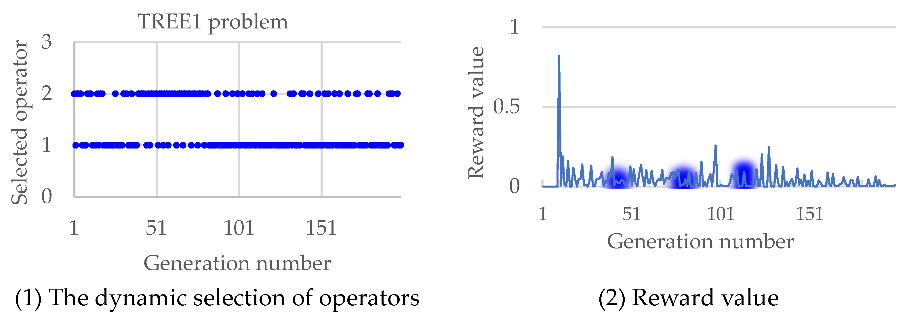
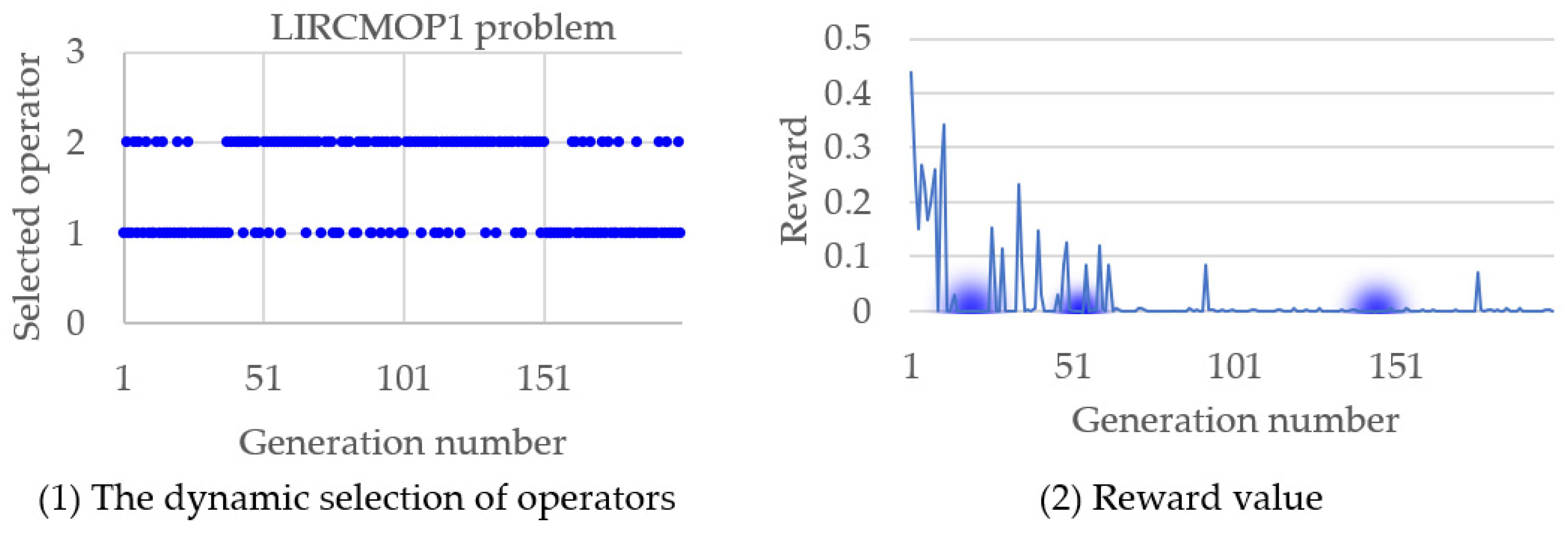
In summary, the autonomous evolution optimization method guided by the population feasibility state is effective in improving the performance of evolutionary algorithms with the constrained method. The autonomy here is the dynamic selection of operators realized by reinforcement learning, as shown in Figure 3 and Figure 4, where the TREE1 and LIRCMOP1 problems are performed as examples, and the variation of reward value along the operator selection is also simulated. In Figure 3, it can be seen that at the three key time points where the operator is preferentially selected, the reward value is obviously improved. A similar phenomenon also happened in Figure 4; at the three key time points where the operator is preferentially selected, the reward value is also obviously improved. Overall, the method proposed in this article can uniformly select operators in the early stages of evolution, accumulating sufficient and evenly distributed sampling data. In the later stage of evolution, this method can continuously adjust the operators adopted to improve the solving performance of the algorithm based on operator evaluation and real-time population state.
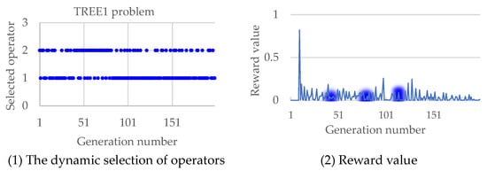
Figure 3.
The selected operators along the evolutionary process and the corresponding reward change in solving the TREE1 problem.
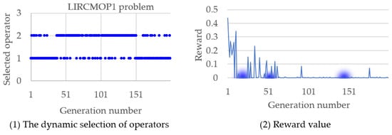
Figure 4.
The selected operators along the evolutionary process and the corresponding reward change in solving the LIRCMOP1 problem.
The demonstrated effectiveness of using reinforcement learning to autonomously select multiple operators in conjunction with the constrained method can be explained as follows:
- (1)
- Collaboration of multiple operators can increase the population diversity. When solving constrained multi-objective optimization problems, the complexity of the problem often leads to the algorithm falling into local optima. By using multiple operators to work together, the population diversity is increased, thereby enlarging the coverage on search space, and helping to avoid getting stuck in local optima.
- (2)
- Multiple operators’ collaboration can improve the convergence speed of algorithms. When solving constrained multi-objective optimization problems, the algorithm needs to find the optimal solution within a limited number of iterations. By using multiple operators to work together, it is possible to search in different directions, thereby accelerating the convergence speed of the algorithm.
- (3)
- Collaboration of multiple operators can increase the search ability of algorithms. When solving constrained multi-objective optimization problems, the algorithm needs to find the optimal solution in the search space. By using multiple operators to work together, it is possible to search in different directions simultaneously, thereby increasing the search capability of the algorithm and helping to find better solutions.
4.5. The Comprehensive Performance of the Proposed Method
4.5.1. Compared with State-of-the-Art Constrained Optimization Algorithms
This section selects the state-of-the-art constrained multi-objective optimization algorithms—including CMOEA-MS, BiCo, AGE-MOEA-II, DSPCMDE, and the classic algorithm NSGA-II—to compare with IDCNSGA-III. Regarding the test problems, IDCNSGA-III and the selected comparative algorithms were independently run 30 times, obtaining HV indicator values. The performance statistics of HV are presented in Table 2 and Table 3, where the best results are highlighted.
Table 2.
HV indicator statistics for IDNSGA-III and comparison algorithms (part 1).
Table 3.
HV indicator statistics for IDNSGA-III and comparison algorithms (part 2).
The problems in the TREE test set have a high dimensionality, making them challenging to solve. In comparison with other algorithms, IDCNSGA-III has achieved significant advantages. This may be attributed to the fact that, although the test problems have high dimensions, the fitness landscape is relatively simple, and the gradient information is clear. The algorithm can effectively utilize feedback information, promoting rapid convergence of the population.
The feasible regions of the LIR-CMOP test suite are small. For some test problems, the constrained Pareto front exhibits sparse points, continuous segments, and discontinuous segments. A portion of the feasible region has closed, non-closed, and three-dimensional grid shapes. For the two-dimensional test problems, such as LIR-CMOP1 to LIR-CMOP12, IDCNSGA-III exhibits a clear advantage over the CMOEA-MS, BiCo, AGEMOEA-II, and NSGA-II algorithms in the comparison. There is no clear advantage over DSPCMDE in the comparison. Particularly in the two three-dimensional problems, LIR-CMOP13 to LIR-CMOP14, the performance is not satisfactory. This could be due to the fact that when the algorithm executes a certain operator and receives a higher reward, its inherent greediness favors continuously executing a single operator, leading to premature convergence of the population. Moreover, in high-dimensional problems, which have more local optima, the greediness issue of the algorithm becomes more pronounced.
For the MW test problems, the constraints have various forms. In general, the feasible region is very small, and it is divided from a very large infeasible region. Hence, the constrained Pareto front includes multiple isolated solutions. Overall, IDCNSGA-III exhibits a relatively significant advantage compared with the CMOEA-MS, AGEMOEAII, DSPCMDE, and NSGA-II algorithms. In comparison with BiCo, IDCNSGA-III shows a slight performance deficiency when facing problems with non-contiguous, narrow, and scattered constraint shapes such as MW2, MW6, and MW10. This may happen due to the dependence on well-defined infeasible solutions to provide the information guiding population evolution. The scattered, narrow, and non-contiguous nature of the constraint regions may lead to insufficient feedback information, thus limiting its regulatory effect.
In addition, a Friedman test is used to rank all the algorithms. As the ranking results presented in Table 4, IDCNSGA-III shows the best ranking, and shows significant advantages in comparison with other algorithms.
Table 4.
Average rankings of the algorithms with Friedman test.
In summary, when compared with other algorithms, the proposed method in this paper has the best performance. This further elucidates the effectiveness of the proposed approach. In terms of the problem dimension, the dimensions of TREE problems are higher than 100, where IDCNSGA-III has more significant advantages than other algorithms. The possible explanation is that combining the constrained method and the multi-operator method can fully leverage the advantages of both methods. Loosening the constraints first and gradually tightening them can effectively reduce the search space and improve search efficiency. In addition, the multi-operator method can search the solution space more comprehensively and improve search quality. The comprehensive application of the two methods can better balance search efficiency and search quality, thereby exhibiting better performance in solving high-dimensional problems.
4.5.2. Compared with -Feasibility-Based Constrained Optimization Algorithms
Because our algorithm uses the -feasibility-based population state to guide the evolution, we need to compare other -feasibility-based constrained optimization algorithms to show the advantages. The selected state-of-the-art competitors include Trip, DPPPS, and CAEAD. For the test problems, as well as TREE, LIRCMOP, and MW, we also selected the RWMOP test suite to deeply test the performance of all algorithms. These problems are classified into five parts according to their domain: mechanical design problems; chemical engineering problems; process design and synthesis problems; power electronics problems; and power system problems. According to Kumar et al.’s analysis, the RWMOP test function contains various questions with different difficulty levels. Although the RWMOP benchmark suite contains testing issues with relatively low dimensions (up to 34), most problems are hard to solve with the most advanced algorithms. IDCNSGA-III and the selected comparative algorithms were independently run 30 times, obtaining HV indicator values. The performance statistics of HV are presented in Table 5, where the best results are highlighted, and the results for all algorithms that cannot find feasible solutions are removed. All the problems for which no single algorithm can find a feasible solution are removed from Table 5.
Table 5.
HV indicator statistics for IDNSGA-III and comparison algorithms.
The experimental results illustrate that IDCNSGA-III has significant advantages in comparison with competitors. For problems TREE3 to LIRCMOP6, and MW9-MW14, IDCNSGA-III has the most prominent performance. Specifically, IDCNSGA-III achieved “34+/14−/7=”, “36+/14−/5=” and “37+/13−/5=” on all test problems. In each test suite, for all existing problems IDCNSGA-III can find feasible solutions, while competitors cannot make it. Particularly in the MW test suite, there were five problems that competitors could not solve even one of. This indicates that our proposed algorithm is efficient and has promising performance in terms of applying -feasibility techniques.
4.5.3. Sensitivity Analysis of Key Parameters
To better set the parameters in our algorithm, the influence of key parameters on algorithm performance are tested with different parameters setting. , , and control the update of current reward to Q-table, prediction ability of reward, and greedy, respectively. Hence, we set the value of with 0.001, 0.005, 0.01, 0.015, and 0.02, respectively. changes from 0.1 to 0.5 with an interval of 0.1, changes from 0.5 to 0.9 with an interval of 0.1. Each version of IDCNSGA-III is run 30 times on MW, LIRCMOP, and TREE test suites independently. All versions of IDCNSGA-III are compared with each other using Friedman test, and the ranking results of IDCNSGA-III on , , and are presented in Table 6, Table 7 and Table 8, respectively. For , = 0.005 has the best ranking, while = 0.001 and = 0.01 have similar performance. That means = 0.005 is a promising setting. For , a relatively small setting is better. = 0.2 shows the best performance than = 0.3, 0.4, and 0.5. For , = 0.8 is a good choice, which surpasses = 0.5, 0.6, 0.7, and 0.9.
Table 6.
Average rankings of the algorithms with different value (Friedman).
Table 7.
Average rankings of the algorithms with different value (Friedman).
Table 8.
Average rankings of the algorithms with different value (Friedman).
5. Conclusions
We propose a population feasibility state guided autonomous evolutionary optimization method for handling constrained multi-objective optimization problems. Taking DCNSGA-III as an example, our proposed method significantly improves its performance on four test suites, demonstrating the effectiveness of our approach. In addition, the comparison of IDCNSGA-III with five state-of-the-art constrained multi-objective optimization algorithms and three -feasibility based constrained multi-objective optimization algorithms also demonstrates the effectiveness of our approach. The significant performance of the RWMOP benchmark suite illustrate the scalability of our algorithm in dealing with real-world problems.
However, our method does not significantly improve the performance of the embedded algorithm for test problems with high-dimensional objectives and non-closed constraint shapes. To further enhance performance, we will investigate the following issues in our future work: (1) Designing new methods for describing population state. (2) Integrating new reproduction operator.
Author Contributions
Conceptualization, M.Z.; methodology, M.Z.; software, M.Z.; validation, M.Z.; formal analysis, M.Z.; investigation, M.Z.; resources, M.Z.; data curation, M.Z. and Y.X.; writing—original draft preparation, M.Z. and Y.X.; writing—review and editing, M.Z. and Y.X.; visualization, M.Z. and Y.X.; supervision, M.Z.; project administration, M.Z.; funding acquisition, M.Z. All authors have read and agreed to the published version of the manuscript.
Funding
This research was funded by the National Natural Science Foundation of China with grant No. 62303465, the Shandong Provincial Natural Science Foundation with grant No. ZR2022LZH017.
Data Availability Statement
The data presented in this study are available on request from the corresponding author.
Conflicts of Interest
The authors declare no conflicts of interest.
References
- Hu, H.; Sun, X.; Zeng, B.; Gong, D.; Zhang, Y. Enhanced evolutionary multi-objective optimization-based dispatch of coal mine integrated energy system with flexible load. Appl. Energy 2022, 307, 118130. [Google Scholar] [CrossRef]
- Gong, D.; Xu, B.; Zhang, Y.; Guo, Y.; Yang, S. A Similarity-Based Cooperative Co-Evolutionary Algorithm for Dynamic Interval Multiobjective Optimization Problems. IEEE Trans. Evol. Comput. 2020, 24, 142–156. [Google Scholar] [CrossRef]
- Zuo, M.; Dai, G.; Peng, L.; Wang, M.; Liu, Z.; Chen, C. A case learning-based differential evolution algorithm for global optimization of interplanetary trajectory design. Appl. Soft Comput. 2020, 94, 106451. [Google Scholar] [CrossRef]
- Kumar, A.; Wu, G.H.; Ali, M.Z.; Mallipeddi, R.; Suganthan, P.N.; Das, S. A test-suite of non-convex constrained optimization problems from the real-world and some baseline results. Swarm Evol. Comput. 2020, 56, 100693. [Google Scholar] [CrossRef]
- Liang, J.; Ban, X.; Yu, K.; Qu, B.; Qiao, K.; Yue, C.; Chen, K.; Tan, K.C. A Survey on Evolutionary Constrained Multiobjective Optimization. IEEE Trans. Evol. Comput. 2023, 27, 201–221. [Google Scholar] [CrossRef]
- Zuo, M.C.; Dai, G.M.; Peng, L.; Tang, Z.; Gong, D.W.; Wang, Q.X. A differential evolution algorithm with the guided movement for population and its application to interplanetary transfer trajectory design. Eng. Appl. Artif. Intell. 2022, 110, 104727. [Google Scholar] [CrossRef]
- Zuo, M.C.; Dai, G.M.; Peng, L. A new mutation operator for differential evolution algorithm. Soft Comput. 2021, 25, 13595–13615. [Google Scholar] [CrossRef]
- Zuo, M.C.; Dai, G.M.; Peng, L. Multi-agent genetic algorithm with controllable mutation probability utilizing back propagation neural network for global optimization of trajectory design. Eng. Optim. 2019, 51, 120–139. [Google Scholar] [CrossRef]
- Jiao, L.C.; Luo, J.J.; Shang, R.H.; Liu, F. A modified objective function method with feasible-guiding strategy to solve constrained multi-objective optimization problems. Appl. Soft Comput. 2014, 14, 363–380. [Google Scholar] [CrossRef]
- Maldonado, H.M.; Zapotecas-Martínez, S. A Dynamic Penalty Function within MOEA/D for Constrained Multi-objective Optimization Problems. In Proceedings of the 2021 IEEE Congress on Evolutionary Computation (CEC), Kraków, Poland, 28 June–1 July 2021; pp. 1470–1477. [Google Scholar]
- Fan, Z.; Ruan, J.; Li, W.J.; You, Y.G.; Cai, X.Y.; Xu, Z.L.; Yang, Z.; Sun, F.Z.; Wang, Z.J.; Yuan, Y.T.; et al. A Learning Guided Parameter Setting for Constrained Multi-Objective Optimization. In Proceedings of the 2019 1st International Conference on Industrial Artificial Intelligence, Shenyang, China, 22–26 July 2019. [Google Scholar]
- Morovati, V.; Pourkarimi, L. Extension of Zoutendijk method for solving constrained multiobjective optimization problems. Eur. J. Oper. Res. 2019, 273, 44–57. [Google Scholar] [CrossRef]
- Schütze, O.; Alvarado, S.; Segura, C.; Landa, R. Gradient subspace approximation: A direct search method for memetic computing. Soft Comput. 2017, 21, 6331–6350. [Google Scholar] [CrossRef]
- Long, Q. A constraint handling technique for constrained multi-objective genetic algorithm. Swarm Evol. Comput. 2014, 15, 66–79. [Google Scholar] [CrossRef]
- Vieira, D.A.G.; Adriano, R.L.S.; Vasconcelos, J.A.; Krähenbühl, L. Treating constraints as objectives in multiobjective optimization problems using niched pareto genetic algorithm. IEEE Trans. Magn. 2004, 40, 1188–1191. [Google Scholar] [CrossRef]
- Ming, F.; Gong, W.; Wang, L.; Gao, L. Constrained Multi-objective Optimization via Multitasking and Knowledge Transfer. In Proceedings of the IEEE Transactions on Evolutionary Computation, Online, 20 December 2022. [Google Scholar]
- Deb, K.; Pratap, A.; Agarwal, S.; Meyarivan, T. A fast and elitist multiobjective genetic algorithm: NSGA-II. IEEE Trans. Evol. Comput. 2002, 6, 182–197. [Google Scholar] [CrossRef]
- Takahama, T.; Sakai, S. Constrained optimization by the ε constrained differential evolution with gradient-based mutation and feasible elites. IEEE Congr. Evol. Comput. 2006, 3, 2322–2327. [Google Scholar]
- Runarsson, T.P.; Xin, Y. Stochastic ranking for constrained evolutionary optimization. IEEE Trans. Evol. Comput. 2000, 4, 284–294. [Google Scholar] [CrossRef]
- Saha, A.; Ray, T. Equality Constrained Multi-Objective Optimization. In Proceedings of the IEEE Congress on Evolutionary Computation, Brisbane, QLD, Australia, 10–15 June 2012. [Google Scholar]
- Hamida, S.B.; Schoenauer, M. ASCHEA: New results using adaptive segregational constraint handling. In Proceedings of the 2002 Congress on Evolutionary Computation. CEC’02, Honolulu, HI, USA, 12–17 May 2002; pp. 884–889. [Google Scholar]
- Zapotecas-Martínez, S.; Ponsich, A. Constraint Handling within MOEA/D Through an Additional Scalarizing Function. Genet. Evol. Comput. Conf. 2020, 6, 595–602. [Google Scholar]
- Liu, Z.Z.; Wang, Y.; Wang, B.C.A. Indicator-Based Constrained Multiobjective Evolutionary Algorithms. IEEE Trans. Syst. Man Cybern.-Syst. 2021, 51, 5414–5426. [Google Scholar] [CrossRef]
- Jan, M.A.; Khanum, R.A. A study of two penalty-parameterless constraint handling techniques in the framework of MOEA/D. Appl. Soft Comput. 2013, 13, 128–148. [Google Scholar] [CrossRef]
- Ying, W.Q.; Peng, D.X.; Xie, Y.H.; Wu, Y. An Annealing Stochastic Ranking Mechanism for Constrained Evolutionary Optimization. In Proceedings of the 2016 International Conference on Information System and Artificial Intelligence, Hong Kong, China, 24–26 June 2016; pp. 576–580. [Google Scholar]
- Sabat, S.L.; Ali, L.; Udgata, S.K. Stochastic Ranking Particle Swarm Optimization for Constrained Engineering Design Problems; Lecture Notes in Computer Science; Springer: Berlin/Heidelberg, Germany, 2010; 672p. [Google Scholar]
- Li, L.; Li, G.P.; Chang, L. On self-adaptive stochastic ranking in decomposition many-objective evolutionary optimization. Neurocomputing 2022, 489, 547–557. [Google Scholar] [CrossRef]
- Ying, W.Q.; He, W.P.; Huang, Y.X.; Wu, Y. An Adaptive Stochastic Ranking Mechanism in MOEA/D for Constrained Multi-objective Optimization. In Proceedings of the 2016 International Conference on Information System and Artificial Intelligence, Hong Kong, China, 24–26 June 2016; pp. 514–518. [Google Scholar]
- Gu, Q.H.; Wang, Q.; Xiong, N.N.; Jiang, S.; Chen, L. Surrogate-assisted evolutionary algorithm for expensive constrained multi-objective discrete optimization problems. Complex Intell. Syst. 2022, 8, 2699–2718. [Google Scholar] [CrossRef]
- Wang, H.D.; Jin, Y.C. A Random Forest-Assisted Evolutionary Algorithm for Data-Driven Constrained Multiobjective Combinatorial Optimization of Trauma Systems. IEEE Trans. Cybern. 2020, 50, 536–549. [Google Scholar] [CrossRef]
- Li, B.D.; Tang, K.; Li, J.L.; Yao, X. Stochastic Ranking Algorithm for Many-Objective Optimization Based on Multiple Indicators. IEEE Trans. Evol. Comput. 2016, 20, 924–938. [Google Scholar] [CrossRef]
- Chen, Y.; Yuan, X.P.; Cang, X.H. A new gradient stochastic ranking-based multi-indicator algorithm for many-objective optimization. Soft Comput. 2019, 23, 10911–10929. [Google Scholar] [CrossRef]
- Yu, X.B.; Yu, X.R.; Lu, Y.Q.; Yen, G.G.; Cai, M. Differential evolution mutation operators for constrained multi-objective optimization. Appl. Soft Comput. 2018, 67, 452–466. [Google Scholar] [CrossRef]
- Xu, B.; Duan, W.; Zhang, H.F.; Li, Z.Q. Differential evolution with infeasible-guiding mutation operators for constrained multi-objective optimization. Appl. Intell. 2020, 50, 4459–4481. [Google Scholar] [CrossRef]
- Liu, Y.J.; Li, X.; Hao, Q.J. A New Constrained Multi-objective Optimization Problems Algorithm Based on Group-sorting. Proc. Genet. Evol. Comput. Conf. Companion 2019, 7, 221–222. [Google Scholar]
- He, C.; Cheng, R.; Tian, Y.; Zhang, X.Y.; Tan, K.C.; Jin, Y.C. Paired Offspring Generation for Constrained Large-Scale Multiobjective Optimization. IEEE Trans. Evol. Comput. 2021, 25, 448–462. [Google Scholar] [CrossRef]
- Tian, Y.; Li, X.P.; Ma, H.P.; Zhang, X.Y.; Tan, K.C.; Jin, Y.C. Deep Reinforcement Learning Based Adaptive Operator Selection for Evolutionary Multi-Objective Optimization. IEEE Trans. Emerg. Top. Comput. Intell. 2023, 7, 1051–1064. [Google Scholar] [CrossRef]
- Zuo, M.; Gong, D.; Wang, Y.; Ye, X.; Zeng, B.; Meng, F. Process Knowledge-guided Autonomous Evolutionary Optimization for Constrained Multiobjective Problems. IEEE Trans. Evol. Comput. 2023, 28, 193–207. [Google Scholar] [CrossRef]
- Jiao, R.W.; Zeng, S.Y.; Li, C.H.; Yang, S.X.; Ong, Y.S. Handling Constrained Many-Objective Optimization Problems via Problem Transformation. IEEE Trans. Cybern. 2021, 51, 4834–4847. [Google Scholar] [CrossRef]
- Tian, Y.; Cheng, R.; Zhang, X.; Jin, Y. PlatEMO: A MATLAB Platform for Evolutionary Multi-Objective Optimization [Educational Forum]. IEEE Comput. Intell. Mag. 2017, 12, 73–87. [Google Scholar] [CrossRef]
- Kumar, A.; Wu, G.H.; Ali, M.Z.; Luo, Q.Z.; Mallipeddi, R.; Suganthan, P.N.; Das, S. A Benchmark-Suite of real-World constrained multi-objective optimization problems and some baseline results. Swarm Evol. Comput. 2021, 67, 100961. [Google Scholar] [CrossRef]
- Liang, J.; Qiao, K.J.; Yu, K.J.; Qu, B.Y.; Yue, C.T.; Guo, W.F.; Wang, L. Utilizing the Relationship Between Unconstrained and Constrained Pareto Fronts for Constrained Multiobjective Optimization. IEEE Trans. Cybern. 2023, 53, 3873–3886. [Google Scholar] [CrossRef]
- Tian, Y.; Zhang, Y.; Su, Y.; Zhang, X.; Tan, K.C.; Jin, Y. Balancing Objective Optimization and Constraint Satisfaction in Constrained Evolutionary Multiobjective Optimization. IEEE Trans. Cybern. 2022, 52, 9559–9572. [Google Scholar] [CrossRef]
- Liu, Z.Z.; Wang, B.C.; Tang, K. Handling Constrained Multiobjective Optimization Problems via Bidirectional Coevolution. IEEE Trans. Cybern. 2022, 52, 10163–10176. [Google Scholar] [CrossRef]
- Panichella, A. An Improved Pareto Front Modeling Algorithm for Large-scale Many-Objective Optimization. Proc. Genet. Evol. Comput. Conf. 2022, 7, 565–573. [Google Scholar]
- Yu, K.J.; Liang, J.; Qu, B.Y.; Luo, Y.; Yue, C.T. Dynamic Selection Preference-Assisted Constrained Multiobjective Differential Evolution. IEEE Trans. Syst. Man Cybern.-Syst. 2022, 52, 2954–2965. [Google Scholar] [CrossRef]
- Ming, F.; Gong, W.Y.; Wang, L.; Lu, C. A tri-population based co-evolutionary framework for constrained multi-objective optimization problems. Swarm Evol. Comput. 2022, 70, 101055. [Google Scholar] [CrossRef]
- Zou, J.; Sun, R.Q.; Yang, S.X.; Zheng, J.H. A dual-population algorithm based on alternative evolution and degeneration for solving constrained multi-objective optimization problems. Inf. Sci. 2021, 579, 89–102. [Google Scholar] [CrossRef]

Disclaimer/Publisher’s Note: The statements, opinions and data contained in all publications are solely those of the individual author(s) and contributor(s) and not of MDPI and/or the editor(s). MDPI and/or the editor(s) disclaim responsibility for any injury to people or property resulting from any ideas, methods, instructions or products referred to in the content. |
© 2024 by the authors. Licensee MDPI, Basel, Switzerland. This article is an open access article distributed under the terms and conditions of the Creative Commons Attribution (CC BY) license (https://creativecommons.org/licenses/by/4.0/).