A Divestment Model: Migration to Green Energy Investment Portfolio Concept

Abstract

In a targeted terminal wealth generated by bond and risky assets, where the proportion of a risky asset is gradually being phased down, we propose a divestment model in a risky asset compensated by growth in a bond (insurance). The model includes the phase-down rate of the risky asset, ${\displaystyle c\left(t\right),}$ the variable proportion, ${\displaystyle \pi \left(t\right),}$ in a risky asset and the interest rate, ${\displaystyle r,}$ of the bond. To guide the growth of the total wealth in this study, we compared it to the Øksendal and Sulem (Backward Stochastic Differential Equations and Risk Measures (2019)) total wealth for which ${\displaystyle c\left(t\right)=0,}$ and ${\displaystyle \pi \left(t\right)}$ is a constant. We employed the Fokker–Planck equation to find the variable moment, ${\displaystyle \pi \left(t\right),}$ and the associated variance. We proved the existence and uniqueness of the first moment by Feller’s criteria. We have found a pair ${\displaystyle (c^{*}\left(t\right),r^{*})}$ for each ${\displaystyle \pi \left(t\right)}$, which guarantees a growing total wealth. We have addressed the question whether this pair can reasonably be achieved to ensure an acceptable phase-down rate at a financially achievable interest rate, ${\displaystyle r^{*}}$.

1. Introduction

Economic growth is key to sustained job opportunities, improved health facilities and improved infrastructure for growing populations. In Sub-Sahara African as well as developed countries, energy consumption is increasing rapidly [1]. To satisfy the energy demand, new coal-powered electricity generating plants are being constructed or plants that were shut down are being revived. In both urban and rural areas of Sub-Saharan Africa, wood energy needs have increased the cutting down of trees. This has resulted in the magnitude of carbon emissions in the environment to increase. Migration to cleaner energy sources such as renewable energies with the intent to phase down and gradually phase out fossil fuels in the wake of increasing climatic extreme conditions is an urgent matter for our planet. Inevitably, this generates movement of income in the energy sector, and this coupled with urbanization issues such as energy use and pollution is contributing to the climate crises [1]. Renewable sources of energy have been accepted as a solution towards reducing the diffusion and accumulation of greenhouse gases (GHG) in the atmosphere en route to achieve a net-zero GHG emission by 2050. “Phase-down” is herein defined as the gradual elimination of an act of production at different stages of a process. Trencher et al. [2] have reviewed the decarbonization approach and have made recommendations towards advancing Sustainable Development Goals (SDGs) 12 and 13 [3]. Their study pointed out that the approach towards achieving the net-zero GHG should be multi-disciplinary, and that due care must be taken to understand how each country will be impacted by this drastic change. They recommended a different spectrum in the way research is conducted and how the changes are implemented. This holistic approach includes reviewing all policies e.g., mine industry policies, manufacturing policies, policy on policies, socio-economics policies, etc. The importance of their findings include, among other things, understanding the impact that divestment in fossil fuel energy would have on jobs, the cost of the eradication of such processes and the benefits of migration towards achieving SDG 7 [3].

Hyun et. al. [4] investigated plausible decarbonization scenarios of the energy sector for a specified number of power plant stocks in the Republic of Korea by 2050. Depending on the portfolio, their study concluded that the proposed phase-out of coal-fired power plants would inevitably require continued investments in renewables and gas power plants, for a country where, currently, coal and nuclear power account for at least 70% of energy supply. Furthermore, the speed of replacing the existing coal and nuclear power plants could adversely affect investment in other vital areas of the Korean economy such as manufacturing, health, etc., due to redirected investment towards renewable energy.

Globally, energy demand continues to grow in response to rapid economic growth needed to maintain stability of rising energy consumption [5]. Countries like China, Japan and Australia are both producers and consumers of coal. They have continued to construct coal plants for the generation of the needed energy. As countries pledge to divest from fossil fuels to prevent global warming, some countries, particularly in Africa, are increasing the number of coal plants to satisfy the rapidly expanding industries and domestic consumption of energy. Kou et. al. [6] conducted a study on whether China can effectively implement a coal phase-out. The study highlights the difficulties China would experience to preserve industrial output, ensure economic stability and maintain people’s standards of living if it complied with the phase-out requirement. China is in a dilemma: divest quickly and suffer economic decline and political upheaval at home, or divest slowly and face condemnation internationally.

Some countries have set targets to phase out all coal-fired electricity production by 2030 and are building new renewable power plants to ensure reliable electricity supply during and after the transition [7]. Other countries have restructured their energy industries and have reduced their greenhouse gas emissions. Others have increased their reliance on natural gas as a substitute for coal and have set clear climate and energy targets, with no new developments in coal mining [8]. Some African governments have expressed commitment to transition to a cleaner energy mix [9,10]. However, this transition has come at a cost. South Africa, for example, is facing a challenge of electricity supply and demand balance, resulting in power interruptions for several hours [11]. The country heavily relies on coal-fired power generation [12,13], which is experiencing operational challenges arising from aging infrastructure and insufficient maintenance.

Oil exploration and gas extraction have been long-standing activities that have met the global demand for energy [14,15]. Despite the efforts to shift to alternative, green and sustainable energy sources, reliance on hydrocarbons continues to increase [16,17]. Velenturf [18] and Li [19] have revealed that this practice [16,17] heavily contributes to the emission of carbon dioxide (${\displaystyle C{O}_2}$), which has uncontrollable impact on global warming. However, excessive consumption and reliance on fossil fuels is necessary to maintain energy production and economic growth. The quick shift to renewables may not be an option for some countries [20] as the shift could have an adverse impact on their GDPs.

Investment in renewables has the potential to facilitate the transition to new energy sources; however, it is important to consider the potential challenges and complexities that can arise in this shift. In this present paper, we aim to model an investor’s portfolio which consists of migration to cleaner energy supported by the growth of a bond as insurance. We find the optimal phase-down rate and the associated optimal attainable bond interest rate that will compensate for the expected loss. We state the problem clearly in Section 2.

2. Formulation of the Problem

We consider an investment made on a commodity that is being phased down but in a targeted manner to obtain a certain terminal wealth at a set time ${\displaystyle T}$. The investor manages two accounts, a risk-free asset (a bond) and a risky asset (a commodity that is losing value due to the global migration to green energy). The bond acts like an insurance anticipating the loss in the risky asset price. This study is a sequel to the study by Øksendal and Sulem [21], who considered a problem of a self-financing replicating portfolio on a risk free asset, ${\displaystyle S_0\left(t\right)}$, and risky investment, ${\displaystyle S_1\left(t\right)}$, with constant proportions ${\displaystyle \pi }$ in a risky asset and ${\displaystyle (1-\pi )}$ in a bond.

The prices of the investments in [21] were given by:

$$\left\{\begin{array}{cc}\hfill d{S}_0\left(t\right)& =S_0\left(t\right)r\left(t\right)dt;{\displaystyle S_0\left(0\right)=1}\hfill \\ \hfill d{S}_1\left(t\right)& =S_1\left(t\right)[\mu \left(t\right)dt+\sigma \left(t\right)dB\left(t\right)];{\displaystyle S_1\left(0\right)>0}\hfill \end{array}\right.$$

(1)

with ${\displaystyle r\left(t\right)>0,\mu \left(t\right)>0}$ and ${\displaystyle \sigma \left(t\right)>0}$ being adapted bounded processes, and ${\displaystyle B\left(t\right)}$ is the Brownian motion. Their main focus was to find the total wealth and the optimal proportion ${\displaystyle \pi }$ that would generate the total wealth ${\displaystyle Y\left(T\right)=F}$, where ${\displaystyle F\in L^2({\mathcal{F}}_T,P)}$ with ${\displaystyle {\mathcal{F}}_T}$ being the filtration with respect to the probability law ${\displaystyle P}$ of ${\displaystyle Y\left(T\right)}$ at terminal time ${\displaystyle T}$.

2.1. The Divestment Model

In the present problem we consider the system of SDEs given by:

$$\left\{\begin{array}{cc}\hfill d{S}_0\left(t\right)& =S_0\left(t\right)r\left(t\right)dt;{\displaystyle S_0\left(0\right)=1}\hfill \\ \hfill d{S}_1\left(t\right)& =S_1\left(t\right)[(\mu \left(t\right)-c\left(t\right))dt+\sigma \left(t\right)dB\left(t\right)];{\displaystyle S_1\left(0\right)>0}\hfill \end{array}\right.$$

(2)

where ${\displaystyle 0\le c\left(t\right)}$ is the phase-down rate. In the system (2), ${\displaystyle S_0\left(t\right)}$ represents an insurance bond price, ${\displaystyle S_1\left(t\right)}$ denotes the risky price of an asset from which the investor is migrating, and ${\displaystyle B\left(t\right)}$ is the Brownian motion. An example of this is the divestment from fossil fuels discussed in the introduction. Migration from fossil fuels is the international effort of moving money and investments out of climate-unfriendly energy industries and re-investing in renewable energy and other environment-friendly initiatives. In this study, re-investment is accounted for by investing in risk-free assets. The parameters in model (2) are denoted as follows: ${\displaystyle r\left(t\right)}$ is the interest rate of the insurance bond, ${\displaystyle \mu \left(t\right)}$ is the growth rate of the stock, ${\displaystyle \sigma \left(t\right)}$ is the volatility of the stock, ${\displaystyle c\left(t\right)}$ is the phase-down rate, ${\displaystyle r\left(t\right),\mu \left(t\right),c\left(t\right)}$ and ${\displaystyle \sigma \left(t\right)\ne 0}$ being adapted and bounded processes. Since money is being taken out of the stock investment, the problem stated in (2) is pseudo self-financing. We want to find at what bond rate ${\displaystyle r\left(t\right)}$ and phase-down rate ${\displaystyle c\left(t\right)}$ the investor can replicate his original strategy of achieving a terminal wealth ${\displaystyle Y\left(T\right)=F}$, where ${\displaystyle F\in L^2({\mathcal{F}}_T,P)}$ or achieve an investment growing towards ${\displaystyle Y\left(T\right)}$.

The problem considered by Øksendal and Sulem [21] was to find the value of the initial wealth ${\displaystyle Y\left(0\right)=Y_{\pi }\left(0\right)}$ and the optimal value ${\displaystyle \pi }$, the proportion invested in the stock, that would generate a terminal wealth ${\displaystyle Y\left(T\right)=F}$, where ${\displaystyle F\in L^2({\mathcal{F}}_T,P)}$.

For a divestment problem herein, where ${\displaystyle \pi \left(t\right)}$ is continuously changing, the problem is not about finding the optimal value ${\displaystyle \pi \left(t\right)}$ but a continuous investment strategy which ensures at least a growing investment ${\displaystyle Y^d\left(t\right)}$.

Definition 1.

A time homogenous Itô drift diffusion is a process ${\displaystyle {\pi }_t=\pi (t,w):[0,\infty )\times \Omega ⟶\mathbb{R}}$ satisfying a stochastic differential equation of the form

$$\begin{array}{c}\hfill d{\pi }_t=a\left({\pi }_t\right)dt+b\left({\pi }_t\right)d{W}_t,t\ge s,{\pi }_s=\pi .\end{array}$$

(3)

where ${\displaystyle W_t}$ is a 1-dimensional Brownian motion, ${\displaystyle b\left(\pi \right):\mathbb{R}⟶\mathbb{R}}$ and ${\displaystyle a\left(\pi \right):\mathbb{R}⟶\mathbb{R}}$ satisfying the existence theorem stated in Øksendal (chap5) [22]

In this study, we have made the following assumptions:

• A1: We assume that the coefficients of the Itô drift diffusion in Equation (3) obey the Fokker–Planck initial value Cauchy problem,

  $$\begin{array}{c}\hfill \frac{\partial P}{\partial t}=\frac{\partial \left(a\right(\pi \left)P\right)}{\partial \pi }+\frac{1}{2}\frac{{\partial }^2\left(b^2\left(\pi \right)P\right)}{\partial {\pi }^2}.\end{array}$$

  (4)

  Note: There are several forms of the diffusion coefficients ${\displaystyle b^2\left(\pi \right)}$ that have been used in the literature, see for example, Frenkel [23], Goodrich, [24] and Gurol 1978 [25].
• A2: In this study, we have adopted the Gurol 1978 [25] coefficients given below by:

  $$\begin{array}{c}\hfill b\left(\pi \right)=\sqrt{q_1^2{\alpha }^2{\pi }^2+q_2^2},a\left(\pi \right)=\alpha \pi .\end{array}$$

  (5)

Remark 1.

The choice of the diffusion coefficient in (5), ${\displaystyle b\left(\pi \right)}$, is dictated by the need to capture internal market fluctuations of the stock measured by the parameter ${\displaystyle q_1}$ and the variability of the stock generated by the external environment measured by the parameter ${\displaystyle q_2}$. The functions in (5) ensure the existence of a unique global solution almost surely for the statistical moments (see [26]).

In terms of (5), the Fokker–Planck Equation (4) becomes,

$$\begin{array}{c}\hfill \frac{\partial P}{\partial t}=\frac{\partial }{\partial \pi }\left(\alpha \pi P\right)+\frac{1}{2}\frac{{\partial }^2}{\partial {\pi }^2}(q_1^2{\alpha }^2{\pi }^2+q_2^2)P.\end{array}$$

(6)

The Itô drift–diffusion (3) together with the Fokker–Planck Equation (4) with the Gurol 1978 [25] coefficients (5) can be solved for the moments of ${\displaystyle \pi \left(t\right)}$ as shown briefly below.

2.1.1. Derivation of Equations for the Statistical Moments

In order to account for any noise, we define ${\displaystyle W_t^w=(W_1\left(t\right),W_2\left(t\right),......,W_n\left(t\right));0\le t\le T}$. The ${\displaystyle n}$th process ${\displaystyle {\pi }^n\left(t\right)}$ of Equation (3) can be written as

$$\begin{array}{ccc}\hfill d{\pi }_t^n& =& {(a(\pi ,t)dt+b(\pi ,t)d{W}_t)}^n\hfill \\ \hfill & =& [n{\pi }^{n-1}a(\pi ,t)+\frac{1}{2}n(n-1){\pi }^{n-2}{b}^2(\pi ,t)]dt+n{\pi }^{n-1}b(\pi ,t)d{W}_n\left(t\right).\hfill \end{array}$$

(7)

Taking expectation, we obtain

$$\begin{array}{c}\hfill \frac{d}{dt}\mathbb{E}\left[{\pi }^n\left(t\right)\right]=n\mathbb{E}\left[{\pi }^{n-1}a(\pi ,t)\right]+\frac{1}{2}n(n-1)\mathbb{E}\left[{\pi }^{n-2}{b}^2(\pi ,t)\right].\end{array}$$

(8)

Using (3) and (6), we can write down the equations for the first and second moments as follows:

$$\begin{array}{c}\hfill n=1:\frac{d\overline{\pi }}{dt}=-a\overline{\pi },\overline{\pi }=\mathbb{E}\left[{\pi }^n\left(t\right)\right],\end{array}$$

(9)

$$\begin{array}{c}\hfill n=2:\frac{d{\overline{\pi }}^2}{dt}=-2a(1-\frac{a{q}_1^2}{2}){\overline{\pi }}^2+q_2^2.\end{array}$$

(10)

Note the following:

1.

From Equation (9), we can see that the first moment decays exponentially. The investment in the risky asset (fossil fuel investment) declines exponentially, a feature which describes divestment from the stock asset.

2.

From Equation (10), one can find the second moment which provides the reflecting boundaries within which the risky asset must evolve.

Lemma 1.

If the coefficients ${\displaystyle a\left(\pi \right)}$ and ${\displaystyle b\left(\pi \right)}$ given in (5) satisfy Feller’s criteria [26], then the Itô drift–diffusion (3) has a unique global positive solution with probability ${\displaystyle 1.}$

Proof. 

It is obvious that ${\displaystyle b^2\left(\pi \right)=q_1^2{\alpha }^2{\pi }^2+q_2^2>0}$, ${\displaystyle \forall \pi \in \mathbb{R}}$. Hence, Feller’s first criteria (H1) is satisfied. To prove the second criteria ${\displaystyle n=2}$, we note that the integral can be written as

$$\begin{array}{ccc}\hfill {\int }_{x-ϵ}^{x+ϵ}\frac{1+\alpha \pi }{q_1^2{\alpha }^2{\pi }^2+q_2^2}d\pi & =& {\int }_{x-ϵ}^{x+ϵ}\frac{d\pi }{q_1^2{\alpha }^2{\pi }^2+q_2^2}+{\int }_{x-ϵ}^{x+ϵ}\frac{\alpha \pi d\pi }{q_1^2{\alpha }^2{\pi }^2+q_2^2}\hfill \\ \hfill & =& \frac{1}{q_2^2}\left(ta{n}^{-1}\left(\frac{(x+ϵ)q_1\alpha }{q_2}\right)-ta{n}^{-1}\left(\frac{(x-ϵ)q_1\alpha }{q_2}\right)\right)\hfill \\ \hfill & +& \frac{1}{2\alpha q_1^2}(ln\left(q_1^2{\alpha }^2{(x+ϵ)}^2+q_2^2\right)\hfill \\ \hfill & -& ln\left(q_1^2{\alpha }^2{(x-ϵ)}^2+q_2^2\right))+c<\infty .\hfill \end{array}$$

(11)

${\displaystyle \square }$

Since both ${\displaystyle arctan\left(x\right)}$ and ${\displaystyle ln\left(x\right)}$ are bounded functions in the interval ${\displaystyle [x-ϵ,x+ϵ]}$, Feller’s second criteria is satisfied. It follows from Lemma (1) that the moments (9) and (10) are unique regardless of the noise ${\displaystyle W_n\in W_t^w}$ (see Chuang Xu [26] for details).

2.1.2. Derivation of the Total Wealth Equation

Let ${\displaystyle \pi \left(t\right)}$ be a pseudo self-financing portfolio representing a fraction of the total wealth ${\displaystyle Y\left(t\right)=Y_{\pi }\left(t\right)}$ invested in the risky asset which is continuously decreasing (being phased down) in time. The total wealth process ${\displaystyle Y\left(t\right)}$ with respect to (2) still takes the form described in Øksendal and Sulem [21] and is given by:

$$\begin{array}{ccc}\hfill dY\left(t\right)& =& \frac{(1-\pi (t\left)\right)}{S_0\left(t\right)}Y\left(t\right)d{S}_0\left(t\right)+\frac{\pi \left(t\right)Y\left(t\right)}{S_1\left(t\right)}d{S}_1\left(t\right)\hfill \\ \hfill & =& Y\left(t\right)\left[\left\{\right(1-\pi \left(t\right)\left)r\right(t)+\pi \mu (t)-\pi c(t\left)\right\}dt+\pi \sigma \left(t\right)dB\left(t\right)\right].\hfill \end{array}$$

(12)

Let ${\displaystyle F\in L^2({\mathcal{F}}_T,P)}$ be a given target of the value of the investment at the terminal time ${\displaystyle T}$. The problem considered by Øksendal and Sulem [21] was solved for ${\displaystyle c\left(t\right)=0}$, and the initial value of the wealth, ${\displaystyle Y\left(0\right)}$, needed to replicate ${\displaystyle Y\left(T\right)=F}$ was calculated. Since phase-down does not occur instantaneously at ${\displaystyle t=0}$, we assume herein that ${\displaystyle Y\left(0\right)}$ is known from [21]. We want to replicate ${\displaystyle Y\left(T\right)}$ from (12) for a continuously changing portfolio ${\displaystyle \pi \left(t\right)}$ in (3). To generate this problem, we let

$$\begin{array}{c}\hfill Z\left(t\right)=Y\left(t\right)\overline{\pi }\left(t\right)\sigma \left(t\right).\end{array}$$

(13)

Then,

$$\begin{array}{c}\hfill \overline{\pi }\left(t\right)=\frac{Z\left(t\right)}{Y\left(t\right)\sigma \left(t\right)}.\end{array}$$

(14)

Equation (12) becomes

$$\begin{array}{ccc}\hfill dY\left(t\right)& =& Y\left(t\right)\left[\{r\left(t\right)-\frac{r\left(t\right)Z\left(t\right)}{Y\left(t\right)\sigma \left(t\right)}+\frac{Z\left(t\right)}{Y\left(t\right)\sigma \left(t\right)}(\mu \left(t\right)-c\left(t\right))\}\right]dt\hfill \\ \hfill & +& \frac{Y\left(t\right)Z\left(t\right)}{Y\left(t\right)\sigma \left(t\right)}\sigma \left(t\right)d{B}_t\hfill \\ \hfill & =& \{r\left(t\right)Y\left(t\right)+\frac{Z\left(t\right)}{\sigma \left(t\right)}(\mu \left(t\right)-c\left(t\right)-r\left(t\right))\}dt+Z\left(t\right)d{B}_t.\hfill \end{array}$$

(15)

More generally, let

$$\begin{array}{c}\hfill g(t,y,z,w):[0,T]\times \mathbb{R}\times \mathbb{R}\times \Omega ⟶\mathbb{R}\end{array}$$

(16)

be an ${\displaystyle \mathbb{F}\in {\mathcal{L}}^2({\mathcal{F}}_t,P)}$ adapted stochastic process in ${\displaystyle (t,w)}$ for each ${\displaystyle y,z}$. Then the equation

$$\begin{array}{c}\hfill dY\left(t\right)=g(t,Y(t),Z(t),w)dt+Z\left(t\right)dB\left(t\right),0\le t\le 1\end{array}$$

(17)

$$\begin{array}{c}\hfill Y\left(0\right)=ya.s\end{array}$$

(18)

is an SDE in the unknown ${\displaystyle {\mathcal{F}}_t}$ adapted process ${\displaystyle \left(Y\right(t),Z(t\left)\right)}$ (driven by Brownian motion). We define the continuous-time stochastic value process, ${\displaystyle {\left(V\left(t\right)\right)}_{t\ge 0}}$, as the integral of the process ${\displaystyle {\left(Y_t\right)}_{t\ge 0}}$, that is,

$$\begin{array}{c}\hfill V\left(T\right)={\int }_0^{T}Y\left(s\right)ds\end{array}$$

(19)

where ${\displaystyle Y\left(t\right)}$ is the solution of (17).

The Problem: Given the SDE (17) and the initial condition (18), we want to find a pair ${\displaystyle (c^{*},r^{*})\in \Gamma }$, where ${\displaystyle \Gamma }$ is the set of all phase-down strategies ${\displaystyle ((c_1,r_1),(c_2,r_2),.,.)}$, for a time-varying portfolio, ${\displaystyle \pi \left(t\right)}$, given by Equation (9), which yields or at least maintains growth towards the Øksendal and Sulem [21] wealth and to determine the time it takes the wealth to grow towards the total wealth ${\displaystyle V\left(T\right)}$ when the stock is being phased down. However, before calculating the value (19), we want to find the optimal values of ${\displaystyle c}$ which must not be exceeded, the optimal value of ${\displaystyle r\left(t\right)}$ which must be exceeded and the time to maturity of ${\displaystyle V\left(t\right)}$. This problem can be stated precisely as follows:

Theorem 1.

Let ${\displaystyle \Phi (s,y)}$ be the value function and ${\displaystyle (c^{*},r^{*})\in \Gamma }$ an optimal strategy such that,

$$\begin{array}{c}\hfill \Phi (s,y)=\underset{c^{*},r^{*}\in \Gamma }{\sup }J{(s,y)}^{c,r}=J^{c^{*},r^{*}}(s,x).\end{array}$$

(20)

where ${\displaystyle c\left(t\right)\in \mathbb{R},r\in \mathbb{R},t\ge s,w\in \Omega }$ and ${\displaystyle \Gamma }$ is the set of all phase-down strategies. Let the value function ${\displaystyle \Phi (s,y)}$ be of the form

$$\begin{array}{cc}\hfill \Phi (s,y)={\displaystyle \frac{K\left(s\right)y^{\lambda }}{\lambda }},& if\lambda \in \mathbb{R}\setminus \left\{0\right\}.\end{array}$$

(21)

Then the phase-down rate is a function of both ${\displaystyle \pi \left(t\right)}$ and ${\displaystyle r}$ given by

$$\begin{array}{c}\hfill c\left(t\right)=\frac{-\lambda [(1-\pi )r+\pi \mu +\frac{1}{2}{\pi }^2{\sigma }^2]}{\pi [(1-\frac{y}{\lambda })-\lambda +y]}.\end{array}$$

(22)

For a given value of ${\displaystyle \pi \left(t\right)}$ generated by Equation (9), the optimal value ${\displaystyle r\left(t\right)}$ which must be exceeded for the value function ${\displaystyle V\left(T\right)}$ to be achieved can be determined.

Proof. 

Let

$$\begin{array}{c}\hfill {\mathbb{E}}^{s,y}[{\int }_0^{\tau }|f(s,Y_s)|ds+|h(\tau ,Y\tau ){|}_{\tau <\infty }]<\infty \forall s,y\end{array}$$

(23)

with ${\displaystyle f:\mathbb{R}\times \mathbb{R}⟶\mathbb{R}}$, ${\displaystyle h:\mathbb{R}\times \mathbb{R}⟶\mathbb{R}}$ being the cost function and the bequest function, respectively, be continuous functions and ${\displaystyle \tau \le T}$ be the first exit time for the process ${\displaystyle \left\{Y_s^{s,y}\right\}}$. We define the performance function ${\displaystyle J{(s,y)}^{c,r}}$ by

$$\begin{array}{c}\hfill J{(s,y)}^{c,r}={\mathbb{E}}^{s,y}[{\int }_0^{\tau }f(s,Y_s)ds+h{(\tau ,Y\tau )}_{\tau <\infty }]\forall s,y,c.\end{array}$$

(24)

where ${\displaystyle \tau \in [0,T]}$. We want to find the value function ${\displaystyle \Phi (s,y)\in C_0^2(\mathbb{R}\times {\mathbb{R}}^n)}$ satisfying the condition

$$\begin{array}{c}\hfill {\mathbb{E}}^y\left[|\Phi \left(Y_T\right)|+{\int }_0^T\left|\left({\mathcal{L}}^c{\Phi }_s\right)\right|ds\right]<\infty \end{array}$$

(25)

for a stopping time ${\displaystyle T<\infty }$ such that

$$\begin{array}{c}\hfill \underset{c}{\sup }\{f^c\left(y\right)+\left({\mathcal{L}}^c\Phi \right)\left(y\right)\}=0.\end{array}$$

(26)

To find the optimal control ${\displaystyle c^{*}}$, we first solve the equation

$$\begin{array}{c}\hfill f(y,c^{*})+\left({\mathcal{L}}^{c^{*}}\Phi \right)\left(y\right)=0\forall Y_{\pi },c^{*}\in \Gamma .\end{array}$$

(27)

From the wealth Equation (12), we have

$$\begin{array}{c}\hfill \left({\mathcal{L}}^c\varphi \right)\left(y\right)={\Phi }_s(s,y)+{\Phi }_y(s,y)y\{(1-\pi )r+\pi \mu -\pi c\}+\frac{1}{2}{\pi }^2{y}^2{\sigma }^2{\Phi }_{yy}(s,y).\end{array}$$

(28)

Differentiating (26), we obtain the following function for the phase-down rate ${\displaystyle c}$:

$$\begin{array}{ccc}\hfill & & f(s,y,c)=\pi yc{\Phi }_y(s,y).\hfill \end{array}$$

(29)

Without loss of generality, we assume a constant relative risk aversion (CRRA) utility function given by:

$$\begin{array}{c}\hfill U\left(y\right)=\left\{\begin{array}{cc}{\displaystyle \frac{y^{\lambda }}{\lambda }},\hfill & \mathrm{if}\lambda \in \mathbb{R}\setminus \left\{0\right\}\hfill \\ \ln y,\hfill & \mathrm{if}\lambda =0.\hfill \end{array}\right.\end{array}$$

(30)

Note that a similar calculation can be performed for other utility functions. Specifically, we choose the value function ${\displaystyle \Phi (s,y)}$ in (28) of the type

$$\begin{array}{cc}\hfill \Phi (s,y)={\displaystyle \frac{K\left(s\right)y^{\lambda }}{\lambda }},& \mathrm{if}\lambda \in \mathbb{R}\setminus \left\{0\right\}.\end{array}$$

(31)

From (27), (29) and (31), we obtain a time-varying value for ${\displaystyle c\left(t\right)}$ of the type

$$\begin{array}{c}\hfill c\left(t\right)=\frac{-\lambda [(1-\pi )r+\pi \mu +\frac{1}{2}{\pi }^2{\sigma }^2]}{\pi [(1-\frac{y}{\lambda })-\lambda +y]}\end{array}$$

(32)

as stated in the theorem where

$$\begin{array}{c}\hfill ((1-\frac{y}{\lambda })-\lambda +y)\ne 0,\lambda \in \mathbb{R}\setminus \left\{0\right\},\\ \hfill K\left(t\right)=K\left(0\right)exp\{-\lambda t((1-\pi )r+\pi \mu -\pi c+\frac{1}{2}{\pi }^2{\sigma }^2+\frac{\pi yc}{\lambda })\}.\end{array}$$

(33)

Furthermore, ${\displaystyle \pi \left(t\right)}$ is of the form

$$\begin{array}{ccc}\hfill \pi \left(t\right)& =& \frac{{\Phi }_y}{{\Phi }_{yy}}\frac{(r+c-\mu )}{\sigma y}.\hfill \end{array}$$

(34)

then from the first moment in Equations (9), (14) and (34), we arrive at a time-varying proportion ${\displaystyle \pi \left(t\right)}$ of the form,

$$\begin{array}{ccc}\hfill \pi \left(t\right)& =& \frac{{\Phi }_y}{{\Phi }_{yy}}\left(\frac{(r-\mu +c)\pi \left(0\right)e^{-at}}{\sigma z}\right);\mathrm{for}\sigma z\ne 0\hfill \\ \hfill & =& \frac{(\mu -r-c)}{{\sigma }^2(1-\lambda )}.\hfill \end{array}$$

(35)

${\displaystyle \square }$

Since ${\displaystyle \pi }$ depends on ${\displaystyle c}$, we note that any choice of ${\displaystyle \pi }$ will be dependent on the size of ${\displaystyle c,r}$, ${\displaystyle \mu }$ and the sets containing ${\displaystyle \lambda }$. The need for a positive value of ${\displaystyle \pi \left(t\right)}$ leads to the following scenarios:

• If ${\displaystyle (r+c)<\mu }$, then ${\displaystyle \lambda \in (-\infty ,1)\setminus \left\{0\right\}}$.
• If ${\displaystyle (r+c)>\mu }$ for all ${\displaystyle \lambda >1}$ then ${\displaystyle (1-\lambda )<(\mu -r-c)}$.

The conditions above can be used to determine the choice of ${\displaystyle \pi }$ with the desirable properties that we need. We will not focus on the case ${\displaystyle \pi \le 0}$ since our interest is not in short positions in any investment.

Proposition 1.

In a phase-down divestment problem given the value function, ${\displaystyle \Phi (s,y)=\frac{K\left(s\right)y^{\lambda }}{\lambda }}$, the phase-down rate is given by

$$\begin{array}{c}\hfill c\left(t\right)=\frac{-\lambda [(1-\pi )r+\pi \mu +\frac{1}{2}{\pi }^2{\sigma }^2]}{\pi [(1-\frac{y}{\lambda })-\lambda +y]};r,\mu >0,\sigma >0\mathit{and}0<\lambda ,\lambda \ne 1\end{array}$$

(36)

and the investment proportion on the stock is given by

$$\begin{array}{c}\hfill \pi \left(t\right)=\frac{(\mu -r-c)}{{\sigma }^2(1-\lambda )}.\end{array}$$

(37)

3. Results and Simulations

For the chosen parameters in our model (2), we want to demonstrate, with hypothetical examples the evolution of the wealth process, ${\displaystyle Y\left(t\right)}$, for varying phase-down rates, interest rates and volatility.

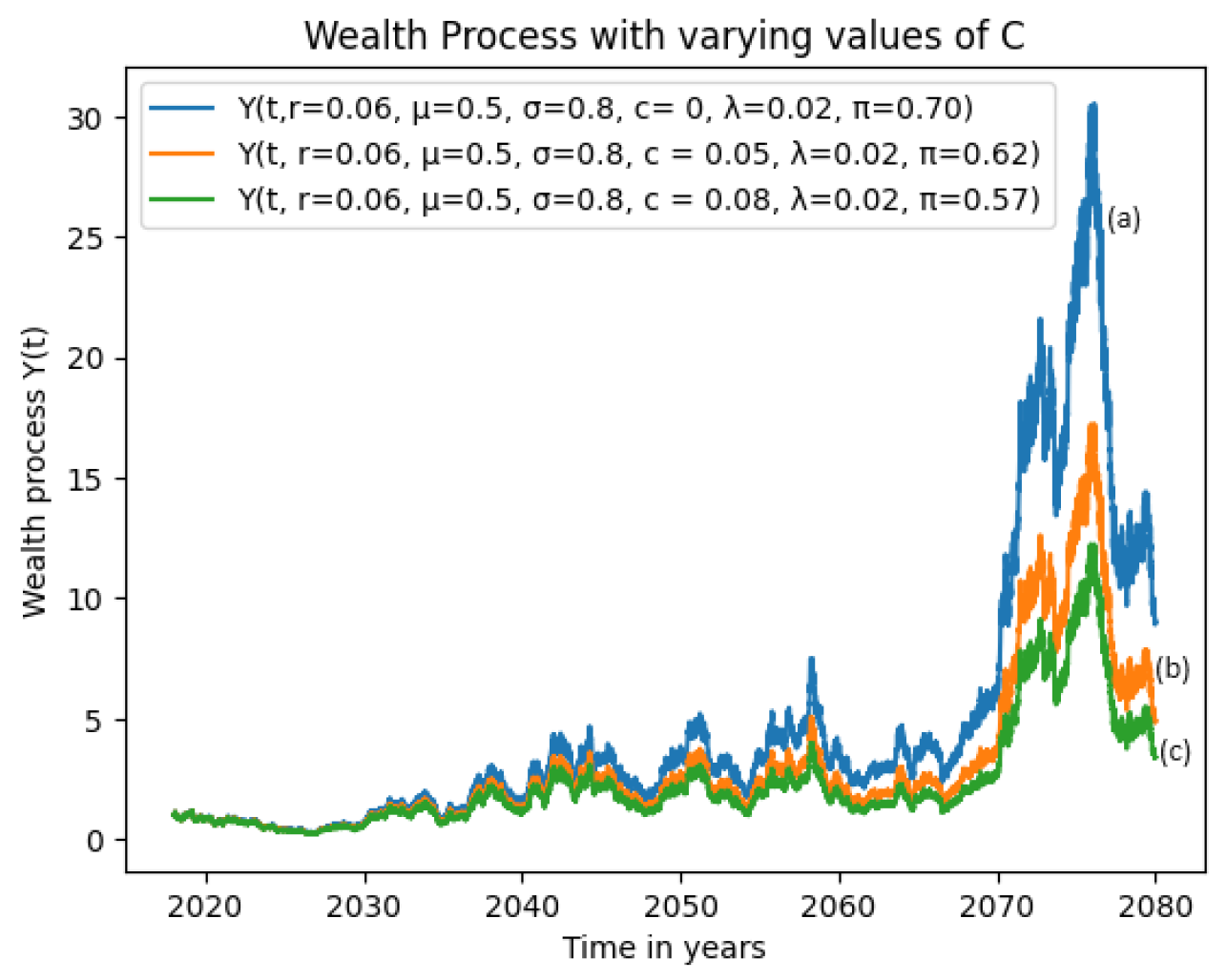
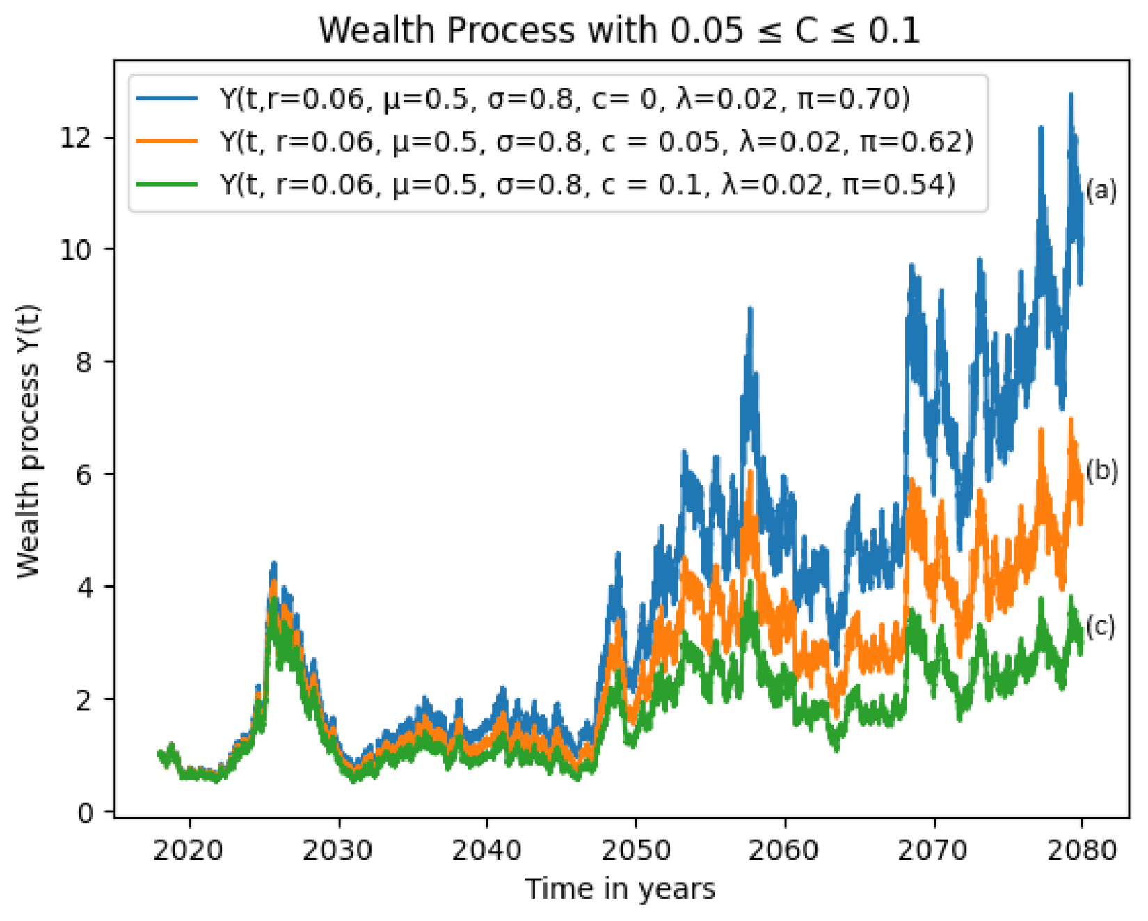
3.1. Hypothetical Examples of Increased Volatility with Varying Phase-Down Rate ${\displaystyle c\left(t\right)}$

3.1.1. Effects of Fixed Interest and Varying Phase-Down Rates

Figure 1 illustrates the progression of the total wealth process, ${\displaystyle Y\left(t\right)}$, for fixed values of the bond interest rate, ${\displaystyle r=0.06}$, the drift of the stock, ${\displaystyle \mu =0.5}$, and the volatility of stock, ${\displaystyle \sigma =0.8}$, for varying values of the phase-down rate, ${\displaystyle c\left(t\right)}$. Figure 1a shows the evolution of ${\displaystyle Y\left(t\right)}$ for ${\displaystyle c\left(t\right)=0}$. This scenario represents the Øksendal and Sulem [21] wealth for a fixed portfolio ${\displaystyle \pi =0.7015}$ (calculated from (37)). Figure 1b,c show the growth of the total wealth for non-zero phase-down rates ${\displaystyle c\left(t\right)=0.05}$ and ${\displaystyle c\left(t\right)=0.08}$, respectively. We can see that the wealth processes, for these phase-down rates, grow more slowly than the Øksendal and Sulem [21] wealth. From Equation (37), the proportions invested in the stock decrease from ${\displaystyle \pi =0.715}$ for ${\displaystyle c\left(t\right)=0}$ to ${\displaystyle \pi =0.6218}$ and ${\displaystyle \pi =0.5740}$ for ${\displaystyle c\left(t\right)=0.05}$ and ${\displaystyle c\left(t\right)=0.08}$, respectively. Clearly, as the phase-down rate increases, the contribution to the wealth from the stock declines (by virtue of 9) and it decreases significantly compared to [21] as the phase-down rate ${\displaystyle c\left(t\right)}$ increases. This observation is supported by Figure 2b,c, for the same values of ${\displaystyle r,\mu }$ and ${\displaystyle \sigma }$ but for a higher value of ${\displaystyle c\left(t\right)=0.1}$. In this case, the total wealth process decreases even further and the stock proportion, too, decreases to ${\displaystyle \pi =0.5421}$. The total wealth processes in Figure 1 and Figure 2 are not targeted wealth processes.

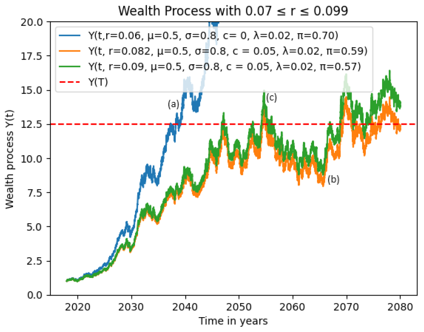
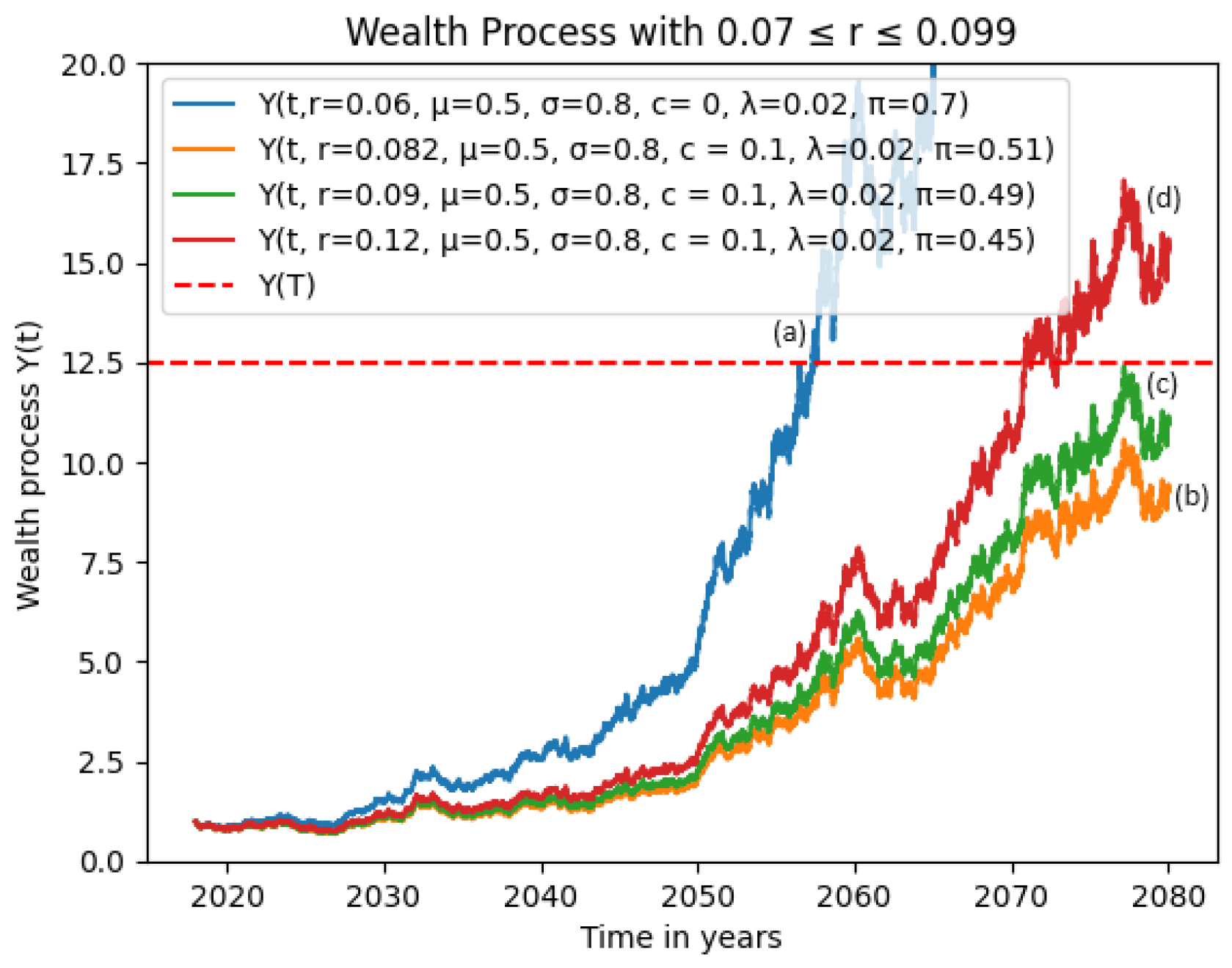
3.1.2. Effects of High Interest Rate

Figure 3 and Figure 4 represent targeted investments designed to achieve a hypothetical terminal wealth, ${\displaystyle Y\left(T\right)=12.5}$, chosen arbitrarily to demonstrate the dynamics of our model. In Figure 3, we fix the drift at ${\displaystyle \mu =0.5}$, the volatility at ${\displaystyle \sigma =0.8}$ (as in Figure 1 and Figure 2), and the phase-down rate at ${\displaystyle c\left(t\right)=0.05}$ as in Figure 1b and Figure 2b, but varied the interest rates. Clearly, the Øksendal and Sulem [21] wealth, in both Figure 3 and Figure 4 outperforms the total wealth for ${\displaystyle c\left(t\right)\ne 0}$ even though the bond interest rate for [21] is lower than that for the cases ${\displaystyle c\left(t\right)=0.05}$ and ${\displaystyle c\left(t\right)=0.1}$. The target wealth in Figure 3 is achieved much earlier for ${\displaystyle c\left(t\right)=0}$ than for ${\displaystyle c\left(t\right)\ne 0}$, which is reached much later for the cases ${\displaystyle c^{*}\left(t\right)=0.05, r^{*}=0.082}$ and ${\displaystyle c^{*}\left(t\right)=0.05, r^{*}=0.09}$.

Figure 4 reveals that increasing the divestment rate ${\displaystyle c\left(t\right)}$ delays the achievement of the target wealth. Moreover, the target wealth is achieved at higher bond rates. For example, the wealth process which fluctuated about the target wealth for ${\displaystyle c\left(t\right)=0.05}$ and bond interest rate ${\displaystyle r=0.09}$, mimicking the Ornstein–Uhlenbeck process, decreases below the target wealth when ${\displaystyle c\left(t\right)}$ is increased to ${\displaystyle 0.1}$ (Figure 4). Furthermore, we have found that for the same phase-down rate ${\displaystyle c\left(t\right)=0.1}$, the target wealth is attained at a higher bond interest rate of ${\displaystyle r=0.12}$. We can see from Figure 3 and Figure 4 that the investment strategies in Figure 3b,c which appeared to be doing well as per the strategy when the divestment rate was ${\displaystyle c\left(t\right)=0.05}$, were not sustainable as shown in Figure 4b,c when the phase-down rate increases to ${\displaystyle c\left(t\right)=0.1}$. Caution must be exercised because changes in the phase-down rate can lead to a change in the viability of the investment.

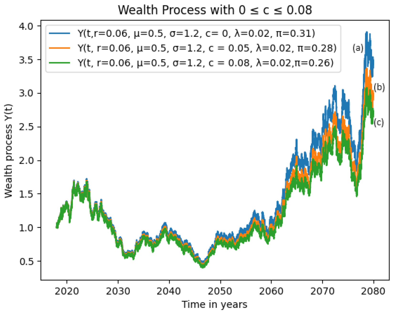
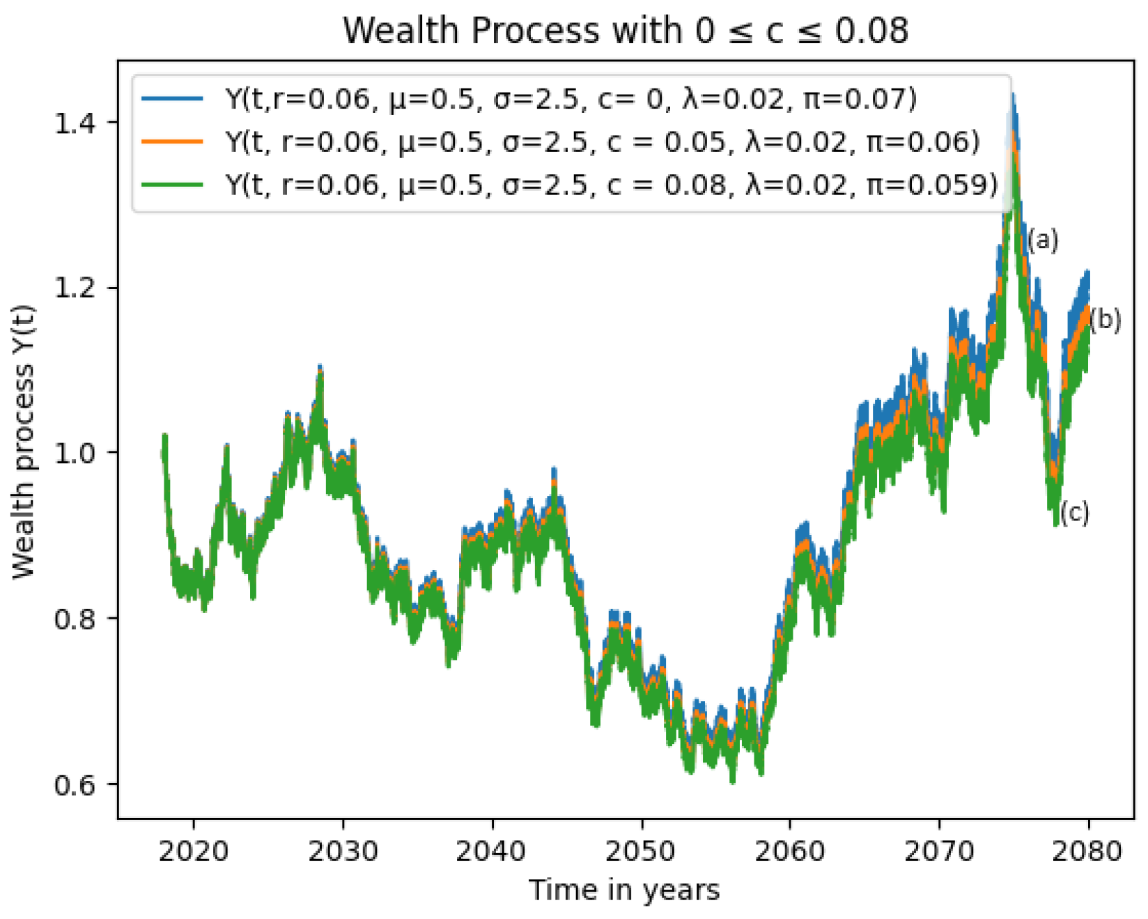
3.1.3. Effects of High Volatility

Figure 5 and Figure 6 show what happens in a highly volatile market when ${\displaystyle r}$ and ${\displaystyle \mu }$ are fixed, as in Figure 3 and Figure 4, but ${\displaystyle c\left(t\right)}$ and ${\displaystyle \sigma }$ are varied. We can see that increasing the volatility has the effect of decreasing the stock proportion. For example, in our case (Figure 5 and Figure 6), the proportion of the stock decreased from ${\displaystyle \pi =0.27636}$ when ${\displaystyle \sigma =1.2}$ to ${\displaystyle \pi =0.06367}$ when ${\displaystyle \sigma =2.5}$. The total wealth process, ${\displaystyle Y\left(t\right)}$, under these circumstances does not grow but instead mimics an Ornstein–Uhlenbeck process with a mean significantly lower than the targeted wealth.

4. Conclusions and Discussion

It is clear from our results that divestment from fossil fuel stocks can be compensated by high bond yields. However, the interest rates for the bonds of over ${\displaystyle 9\%}$ appear to be unrealistic. In Botswana, typical government bond rates are of the order of ${\displaystyle 6\%}$, the value we have used to simulate the case ${\displaystyle c\left(t\right)=0.}$ High volatility is inevitable under the current climatic conditions. Droughts will affect water levels in the dams and lakes, and consequently the hydro-generation capacity. Furthermore, droughts will reduce crop yields and lead to reduced investment in renewables to food imports. The implication of this is that most developing countries will rely on external financial inducement to grow the renewable energy sector. This study has not even taken into account the cost of training and retraining skilled human resources to develop and maintain the newer technologies. There is no doubt that the cost of training and retraining will constrain further the growth of the economies of most developing countries.

This model has demonstrated that the targeted wealth under the unclean energy era can be replicated albeit at higher bond interest rates, which may be unrealistic. However, it will take stricter commitment to the pledges being made by wealthier countries to subsidize the clean energy industry in developing countries. The instability being experienced (wars, droughts, etc.) has made some Western countries revert to fossil fuels such as coal to meet shortages in energy needs. Some Western countries are even encouraging some African coal and oil producers to increase production of these commodities. If this trend continues, it will not be easy to reverse the GHG accumulation after the current instabilities are resolved. The delay in attending to the reduction of carbon and methane accumulation could lead to catastrophic events globally in the near future. It is important in the near future to conduct a comparative study to investigate how developing and developed countries will be impacted separately.

References

1. Das, R.C.; Chatterjee, T.; Ivaldi, E. Co-movements of income and urbanization through energy use and pollution: An investigation for world’s leading polluting countries. Ecol. Indic. 2023, 153, 110381. [Google Scholar] [CrossRef]
2. Trencher, G.; Rinscheid, A.; Rosenbloom, D.; Truong, N. The rise of phase-out as a critical decarbonisation approach: A systematic review. Environ. Res. Lett. 2022, 17, 123002. [Google Scholar] [CrossRef]
3. The Sustainable Development Goals (Sdgs). Available online: https://www.un.org/sustainabledevelopment/sustainable-development-goals/ (accessed on 1 January 2022).
4. Hyun, M.; Cherp, A.; Jewell, J.; Kim, Y.J.; Eom, J. Feasibility trade-offs in decarbonising the power sector with high coal dependence: The case of korea. Renew. Sustain. Energy Transit. 2023, 3, 100050. [Google Scholar] [CrossRef]
5. Zohuri, B.; Mossavar-Rahmani, F.; Behgounia, F. Global electricity demand and clean energy source growth scenario. J. Energy Power Eng. 2022, 16, 156–165. [Google Scholar] [CrossRef]
6. Kou, J.; Sun, F.; Li, W.; Jin, J. Could China declare a “coal phase-out”? an evolutionary game and empirical analysis involving the government, enterprises, and the public. Energies 2022, 15, 531. [Google Scholar] [CrossRef]
7. Cosgrove, A.; Byrne, D.; Khan, F.; Castro, L.; Irwin, S. Air Pollution and Its Impact on the Energy Sector, A Final Report Submitted for the Course SEDV 609, Impact of Proposed Phasing out of Coal-Based Power Plants in Alberta, 16 October 2017. Available online: https://www.researchgate.net/publication/320407265_Impact_of_Proposed_Phasing_Out_of_Coal-Based_Power_Plants_in_Alberta (accessed on 26 February 2022).
8. Hauser, P.; Görlach, B.; Umpfenbach, K.; Perez, R.; Gaete, R. Phasing Out Coal in Chile and Germany. A Comparative Analysis; Agora Energiewende: Berlin, Germany, 2021. [Google Scholar]
9. Liu, X.; Peerally, J.A.; Fuentes, C.D.; Ince, D.; Vredenburg, H. Who makes or breaks energy policymaking in the caribbean small island jurisdictions? a study of stakeholders’ perceptions. Sustainability 2022, 14, 1902. [Google Scholar] [CrossRef]
10. Tesche, M.; Kruger, A. Is the summer season losing potential for solar energy applications in south africa? J. Energy South. 2017, 28, 52–60. [Google Scholar] [CrossRef]
11. Masubelele, M.L.; Masubelele, M.L. Carbon Footprint Assessment in Nature-Based Conservation Management Estates Using South African National Parks as a Case Study. Sustainability 2021, 13, 13969. [Google Scholar] [CrossRef]
12. Lin, S.-J.; Beidari, M.; Lewis, C.E. Energy consumption trends and decoupling effects between carbon dioxide and gross domestic product in south africa. Aerosol Air Qual. Res. 2015, 15, 2676–2687. [Google Scholar] [CrossRef]
13. Nel, E.; Marais, L.; Mqotyana, Z. The regional implications of just transition in the world’s most coal-dependent economy: The case of mpumalanga, south africa. Front. Sustain. Cities 2023, 4, 1059312. [Google Scholar] [CrossRef]
14. Global Oil Supply-and-Demand Outlook to 2040|Mckinsey. Available online: https://www.mckinsey.com/industries/oil-and-gas/our-insights/global-oil-supply-and-demand-outlook-to-2040 (accessed on 26 February 2022).
15. L-Rubaye, A.H.A.; Suwaid, M.A.; Al-Muntaser, A.A.; Varfolomeev, M.A.; Rakhmatullin, I.Z.; Hakimi, M.H.; Saeed, S.A. Intensification of the steam stimulation process using bimetallic oxide catalysts of mfe2o4 (m = cu, co, ni) for in-situ upgrading and recovery of heavy oil. J. Pet. Explor. Prod. Technol. 2021, 12, 577–587. [Google Scholar] [CrossRef]
16. Executive Summary—World Energy Investment 2021—Analysis-Iea. Available online: https://www.iea.org/reports/world-energy-investment-2021/executive-summary (accessed on 1 June 2022).
17. Cockerill, S.; Martin, C. Are Biofuels Sustainable? The eu Perspective. Biotechnol. Biofuels 2008, 1, 9. [Google Scholar] [CrossRef] [PubMed]
18. Velenturf, A.P. A framework and baseline for the integration of a sustainable circular economy in offshore wind. Energies 2021, 14, 5540. [Google Scholar] [CrossRef]
19. Li, D. A Study for Development Suitability of Biomass Power Generation Technology Based on Ghg Emission Reduction Benefits and Growth Potential. Comput. Intell. Neurosci. 2022, 2022, 7961573. [Google Scholar] [CrossRef] [PubMed]
20. Ringim, S.; Alhassan, A.; Güngör, H.; Victor Bekun, F. Economic policy uncertainty and energy prices: Empirical evidence from multivariate dcc-garch models. Energies 2022, 15, 3712. [Google Scholar] [CrossRef]
21. Øksendal, B.; Sulem, A. Backward Stochastic Differential Equations and Risk Measures; Springer: Berlin/Heidelberg, Germany, 2019; pp. 75–91. ISBN 978-1-4939-8930-0. [Google Scholar] [CrossRef]
22. Øksendal, B. Stochastic Differential Equations, 6th ed.; Springer: Berlin/Heidelberg, Germany, 2005; ISBN 978-3-540-04758-2. [Google Scholar] [CrossRef]
23. Frenkel, J. Kinetic Theory of Liquids; Oxford at the Claredon Press: Oxford, UK, 1946. [Google Scholar]
24. Goodrich, F. Nucleation rates and the kinetics of particle growth. i. the pure birth process. Proc. R. Soc. London. Ser. Math. Phys. Sci. 1964, 277, 155–166. [Google Scholar]
25. Gurol, H. Transport Theory Formulation of the Rate Equations, (Univ. of Carlifonia, Santa Barbora). Trans. Am. Nucl. Soc. 1978, 30, 151–159. [Google Scholar]
26. Xu, C. Global threshold dynamics of a stochastic differential equation sis model. J. Math. Anal. Appl. 2017, 447, 736–757. [Google Scholar] [CrossRef]
Figure 1. Wealth process with varying values of c.
Mathematics 12 00915 g001
Figure 2. Wealth process with 0.05 c 0.1 .
Mathematics 12 00915 g002
Figure 3. Wealth process with 0.07 r 0.099 and c = 0.05 .
Mathematics 12 00915 g003
Figure 4. Wealth process with 0.07 r 0.099 and c = 0.1 .
Mathematics 12 00915 g004
Figure 5. Wealth process with 0 c 0.08 and σ = 1.2 .
Mathematics 12 00915 g005
Figure 6. Wealth process with 0 c 0.08 and σ = 2.5 .
Mathematics 12 00915 g006
Disclaimer/Publisher’s Note: The statements, opinions and data contained in all publications are solely those of the individual author(s) and contributor(s) and not of MDPI and/or the editor(s). MDPI and/or the editor(s) disclaim responsibility for any injury to people or property resulting from any ideas, methods, instructions or products referred to in the content.