Distributed Adaptive Tracking Control of Hidden Leader-Follower Multi-Agent Systems with Unknown Parameters

Abstract

The distributed leader-follower control of multi-agent systems is discussed. Each agent is expressed in a discrete-time and non-linear dynamic model with an unknown parameter and can be affected by its neighbors’ history information. For each agent, to identify the parameter, one switching set of the parameter estimates is constructed and the optimal parameter estimate is chosen based on the index switching function. Using the given desired reference signal, the leader agent’s control law is designed, and relying on the neighbors’ history information, each follower agent’s local control law is designed. With the designed distributed tracking adaptive control laws, the whole system tracks the given desired reference signal, and in the face of strong couplings the closed-loop system ultimately reaches an agreement. Finally, by comparing simulations of the control strategy with a normal projection algorithm, the results indicate that the adaptive control method with a switching set of the parameter estimates is effective in improving the control performance.

1. Introduction

Over the past few decades, control strategies for multi-agent systems (MASs) have attracted much interest in different areas, such as unmanned vehicle formation [1,2,3], robotics and sensor networks [4,5,6], spacecraft formation flying [7,8], etc. However, from the viewpoint of control tasks, investigation of the control problem of MASs has mainly considered consistency control [9], cluster control [10], tracking control [11], formation control [12], flocking control [13], and so on.

In an MAS there are many uncertainties. For each agent, it is usually hard and often nearly impossible to create an accurate dynamic model. To deal with the various uncertainties, adaptive control to solve the unknown parameters and structural uncertainties has been studied using different methods [14,15].

Distributed adaptive control [16,17] and centralized adaptive control [18,19] are two important control strategies for MASs. The distributed control strategy uses local information to enable each agent to obtain the local control law. The centralized control strategy assumes that the central station is available and has enough capacity to control all agents. Although the use of these two strategies should be determined depending on the specific circumstances, recently, scholars and researchers have tended to think that the distributed strategy is more promising due to particular restrictions, such as information communication among agents, computational complexity in the theoretical derivation, and so on.

For MASs with a leader or which are leaderless, the adaptive control problem for MASs can be classed into leaderless [20,21] and leader-follower MAS [22,23]. The goal of a leaderless MAS is that all agents’ outputs asymptotically reach the same trajectory, while for the leader-follower MAS, the objective is to enable all agents’ outputs to asymptotically follow a given desired trajectory.

One of the most important topics regarding adaptive control issues of MASs is tracking control [24,25]. Due to the complexity of the performance indices and the interactions among agents, the intrinsic challenges and difficulties regarding the distributed tracking control problem of MASs with uncertainties are discussed. However, many studies have considered distributed tracking control [26,27]. For an MAS with unknown parameters, the parameter estimate is crucial and fundamental. To identify the parameter, various methods have been chosen, such as the projected consensus algorithm [28], the least-squares method [29], the neural network method [30], etc.

As is well-known, the multi-model method is an important technique to identify the parameters for non-linear system control. In the early 1970s, the multi-model method concept was suggested to address the control problem [31]. In [32], for a linear system, a multi-model method based on switching functions was presented, and it was shown that asymptotic tracking in a set of deterministic points could be achieved with unmodeled dynamics.

In [33], a systematic switching control method was used to investigate the adaptive stabilization of a linear time-varying system. In [34], for a discrete-time system, a multi-model method for an adaptive predictive control strategy was adopted switching between the two expressed control laws, which improved the performance of the closed-loop stability.

Most investigations of the multi-model method of adaptive control have focused on handling the various kinds of uncertainties in a single system [35,36,37,38]. In recent years, the distributed multi-model method for adaptive tracking control of MASs has attracted the attention of scholars in the systems and control community [39,40]. For example, in [39], distributed optimal tracking control was investigated based on a correlative measured model.

In light of the above, a multi-model distributed method for the adaptive tracking control of a leader-follower MAS with unknown parameters was investigated. Compared to the projection algorithm described in [41], the multi-model method was used to improve system performance for accelerating parameter convergence. Each agent and its neighbors’ history information influence the outputs. Due to the interactions among agents, the complexity of the performance indices for MAS, and the number of multiple models, certain difficulties and complexities occur. The main results obtained are listed as follows: To identify the parameters, a multi-model method was chosen. The distributed adaptive control scheme was designed based on the equivalence principle. The given desired reference signal and the leader’s control law were designed, and each follower’s local control law was designed according to its neighbors’ history information.

Under the distributed control scheme, each agent follows the given reference signal and the whole system gradually reaches strong synchronization in terms of the mean.

This paper is organized as follows: Section 2 describes the preparatory knowledge and modeling. The projection algorithm and multi-model adaptive method are introduced, and the distributed adaptive parameter update laws are presented in Section 3. Section 4 describes the design of the distributed adaptive control scheme based on the multi-model method. Section 5 provides auxiliary lemmas, and the main theoretical results are presented in Section 6. The simulation results, which show that the adaptive control method with a switching set of the parameter estimates is effective in improving the control performance in comparison with the normal projection algorithm, are presented in Section 7. Section 8 presents the conclusions.

2. Preparatory Knowledge and Modeling

2.1. Graph Theory

In an MAS composed of N agents, each agent through its neighbors’ available information can be connected to other agents. A directed graph $\mathrm{G}=(\mathrm{V},\mathrm{E},\mathrm{A})$ describes the communicated topology among agents. $\mathrm{V}=\{1,2,\cdots ,N\}$ is a vertex set, the ordered edges set $\mathrm{E}=\mathrm{V}\times \mathrm{V}$ means the ordered edges set, and $\mathrm{A}=\left[a_{ij}\right]$ represents an adjacency matrix. The ordered pair $(i,j)$ denotes that the jth agent’s history information has access to the ith agent’s current output.

The jth agent is called by the $i^{th}$ agent’s neighbor.

The adjacency matrix $\left[a_{ij}\right]\in R^{N\times N}$ refers to the matrix whose elements are $a_{ii}=0$, $a_{ij}=0$ if $(i,j)\notin \mathrm{E}$ and $a_{ij}=1$ if $(i,j)\in \mathrm{E}$. ${\mathrm{N}}_i=\{j\in \mathrm{V}|(i,j)\in \mathrm{E}\}$ expresses the $i^{th}$ agent’s all neighbors set. If ${\displaystyle \sum _{j=1}^N}{a}_{ij}\triangleq m_i,i=1,\cdots ,N$, then the diagonal matrix $D=m_1,m_2,\cdots ,m_N$ means an in-degree matrix.

Definition 1

([41,42,43]). If there is a path that follows the direction of the edges of the directed graph such that any two agents i and j are connected, then an adjacency matrix $\mathrm{A}(a_{ij}=0,1)$ is a strongly connected matrix.

Definition 2

([40,41]). If one agent obtains information from the desired reference signal, while the other agents do not know either the existence of the leader or the desired reference signal, then the agent is called a hidden leader.

2.2. Multi-Agent Modeling

In an MAS composed of N agents, the dynamic model of agent i is considered as follows:

$$x_i(T+1)=g_i({\gamma }_i,x_i\left(T\right),{\psi }_i\left(T\right))+u_i\left(T\right),i=1,2,\cdots ,N,$$

(1)

where $x_i(T+1)$ is the output, and $u_i\left(T\right)\in R$ is the input. The time-invariant parameter ${\gamma }_i\in R^{p_i}$ is unknown. ${\psi }_i\left(T\right)$, consisting of the outputs from the $m_i$ neighbors, is an $m_i$-dimensional vector when agent i has $m_i$ neighbors. The mapping $g_i$ is a known non-linear function and is differentiable with respect to the unknown ${\gamma }_i$ function.

Denote the derivative as

$${\mathrm{\Psi }}_i\left(T\right)\triangleq \frac{\partial g_i({\gamma }_i,x_i\left(T\right),{\psi }_i\left(T\right))}{{\partial {\gamma }_i}^{\prime }}{|}_{\gamma ={\widehat{\gamma }}_i\left(T\right)}.$$

In an MAS, to study the adaptive control strategy, the following assumptions are made:

Assumption 1.

In an MAS (1), the adjacency matrix $\mathrm{A}$ is strongly connected.

Remark 1.

This assumption indicates that each agent has received any other agents’ information through directed paths, directly or indirectly.

Assumption 2.

It is reasonable to assume that one or more of the agents are hidden leaders. However, for convenience, the hidden agent assumes that the first agent is a leader.

Assumption 3.

The tracking reference signal sequence $\left\{x^{\ast }\left(T\right)\right\}$ is bounded.

Assumption 4.

The derivative ${\mathrm{\Psi }}_i((x_i\left(T\right),{\psi }_i\left(T\right))$ is a Lipschitz function.

3. Multi-Model Adaptive Method

3.1. The Projection Algorithm

For each agent, in order to provide one of the multiple parameters, the projection algorithm is adopted to estimate the unknown parameters.

A parametric criterion is proposed to estimate the parameter:

$$\begin{array}{cc}\hfill J_i\left({\gamma }_i\right)& =[x_i{(T+1)-g_i({\gamma }_i,x_i\left(T\right),{\psi }_i\left(T\right))-u_i\left(T\right)]}^2+w_i{∥{\gamma }_i-{\widehat{\gamma }}_i\left(T\right)∥}^2,\hfill \end{array}$$

(2)

where $w_i$ is a small positive constant and punishment factor, and ${\widehat{\gamma }}_i\left(T\right)$ is the estimate of ${\gamma }_i$.

For $g_i({\gamma }_i,x_i\left(T\right),{\psi }_i\left(T\right))$ using Taylor’s expansion of function, we obtain

$$\begin{array}{cc}\hfill g_i({\gamma }_i,x_i\left(T\right),{\psi }_i\left(T\right))& \cong g_i({\widehat{\gamma }}_i\left(T\right),x_i\left(T\right),{\psi }_i\left(T\right))+{\mathrm{\Psi }}_i\left(T\right)[{\gamma }_i-{\widehat{\gamma }}_i\left(T\right)].\hfill \end{array}$$

(3)

Plugging (3) into (2), one has

$$\begin{array}{cc}\hfill J_i\left({\gamma }_i\right)& \cong [x_i{(T+1)-g_i({\widehat{\gamma }}_i\left(T\right),x_i\left(T\right),{\psi }_i\left(T\right))-{\mathrm{\Psi }}_i\left(T\right)\times ({\gamma }_i-{\widehat{\gamma }}_i\left(T\right))-u_i\left(T\right)]}^2+w_i{∥{\gamma }_i-{\widehat{\gamma }}_i\left(T\right)∥}^2.\hfill \end{array}$$

Taking the derivative on both sides of (3) and using the minimum value theorem, we can write

$$\begin{array}{c}\hfill \nabla J_i\left({\gamma }_i\right)=0,\end{array}$$

i.e.,

$$\begin{array}{cc}\hfill & [x_i(T+1)-g_i({\widehat{\gamma }}_i\left(T\right),x_i\left(T\right),{\psi }_i\left(T\right))-{\mathrm{\Psi }}_i\left(T\right)({\gamma }_i-{\widehat{\gamma }}_i\left(T\right))-u_i\left(T\right)]\times {\mathrm{\Psi }}_i\left(T\right)-w_i{({\gamma }_i-{\widehat{\gamma }}_i\left(T\right))}^T=0.\hfill \end{array}$$

Rearranging for agent i, we obtain the normal adaptive update law for estimation

$$\begin{array}{cc}\hfill & {\widehat{\gamma }}_i(T+1)={\widehat{\gamma }}_i\left(T\right)+\frac{{\mathsf{\Phi }}_i^T\left(T\right)[x_i(T+1)-{\widehat{x}}_i(T+1)]}{w_i+{∥{\mathrm{\Psi }}_i\left(T\right)∥}^2},\hfill \end{array}$$

(4)

where

$$\begin{array}{c}\hfill {\widehat{x}}_i(T+1)=g_i({\widehat{\gamma }}_i\left(T\right),x_i\left(T\right),{\psi }_i\left(T\right))+u_i\left(T\right).\end{array}$$

In particular, the value ${\widehat{\gamma }}_i(T+1)$ is an on-line estimation after the time-instant $T+1$ and before the time-instant $T+2$. The estimated value ${\widehat{\gamma }}_i(T+1)$ can be used to estimate the output value of the time-instant $T+2$; that is,

$$\begin{array}{c}\hfill {\widehat{x}}_i(T+2)=g_i({\widehat{\gamma }}_i(T+1),x_i(T+1),{\psi }_i\left(T\right))+u_i\left(T\right).\end{array}$$

Remark 2.

In this algorithm, the punishment factor $w_i$ plays a key role. The suitable value $w_i$ is taken to restrict the area of ${\widehat{\gamma }}_i(T+1)-{\widehat{\gamma }}_i\left(T\right)$. And the denominator of (4) is positive when $w_i$ is positive, with no singular case guaranteed.

Remark 3.

For agent i, the estimation is obtained from the recurrence formula by the projection algorithm. ${\widehat{\gamma }}_i\left(T\right)$ is just one of the parameters in the switching set in the time-instant T.

3.2. Multi-Model Adaptive Parameter Estimate

Suppose that each parameter is varying in a given convex set. In other words, the model parameter ${\gamma }_i$ for agent i is unknown, and satisfies ${\gamma }_i\in {\mathrm{\Omega }}_i\subset R^{p_i}$, where ${\mathrm{\Omega }}_i$ is one given nonempty convex set. The set ${\mathrm{\Omega }}_i$ has the following segmentations:

(1)

${\mathrm{\Omega }}_{is}\subset {\mathrm{\Omega }}_i,{\mathrm{\Omega }}_i\ne ⌀,s=1,2,\cdots ,d_i$;

(2)

${\mathrm{\Omega }}_i={\displaystyle {\displaystyle \bigcup }_{s=1}^{d_i}}{\mathrm{\Omega }}_{is}$;

(3)

For ${\mathrm{\Omega }}_{is}(s=1,2,\cdots ,d_i)$, let ${\gamma }_{is}$ and $r_{is}\ge 0$ represent the centre and radius of ${\mathrm{\Omega }}_{is}$, respectively, that is to say, ${\gamma }_{is}\in {\mathrm{\Omega }}_{is}$, and for any ${\gamma }_i\in {\mathrm{\Omega }}_{is}$, one has

$$∥{\gamma }_i-{\gamma }_{is}∥\le r_{is}.$$

(5)

Considering (1) and (4), based on multiple fixed invariant parameters, one has

$${\widehat{\gamma }}_{is}\left(T\right)={\gamma }_{is},s=1,2,\cdots ,d_i.$$

(6)

It is easy to see that one set of multiple parameters is established for agent i. Using the projection parameter update law (4), for the dynamics Equation (1), the normal adaptive parameter model is established. Denoting the normal adaptive model parameter ${\widehat{\gamma }}_{i_1}$ as ${\widehat{\gamma }}_{i,d_i+1}$, we can write

$${\widehat{\gamma }}_{i,d_i+1}\left(T\right)={\widehat{\gamma }}_{i_1}\left(T\right),$$

(7)

where ${\widehat{\gamma }}_{i_1}\left(T\right)$ is obtained from the normal update law (4). Accelerating the parameter convergence to improve the control performance, we bring in another adaptive model parameter ${\widehat{\gamma }}_{i_2}$, whose initial value would be adaptively adjusted to the nearest model parameter of the dynamics. Let

$${\widehat{\gamma }}_{i,d_i+2}\left(T\right)={\widehat{\gamma }}_{i_2}\left(T\right).$$

(8)

Thus, based on (4), (7), and (8), it is easy to establish the multiple parameters’ switching set with $d_i+2$ elements. We can establish the $d_i+2$ models, and the $d_i$ models of them are fixed; the other two models are adaptive models.

The adaptive multiple models are constructed as follows:

$$\begin{array}{cc}\hfill {\widehat{x}}_{is}(T+1)& =g_i({\widehat{\gamma }}_{is},x_i\left(T\right),{\psi }_i\left(T\right))+u_i\left(T\right),i=1,2,\cdots ,N,\hfill \\ \hfill s& =\{1,2,\cdots ,d_i,d_i+1,d_i+2\}.\hfill \end{array}$$

Remark 4.

$(d_i+2)$ models of agent i are established. Obviously, the number of all models of N agents is ${\displaystyle {\displaystyle \sum }_{i=1}^N}(d_i+2)$, which is the number of all models for the whole system.

For agent i, in the $(d_i+2)$ parameters, the question is how to choose the optimal parameter, rapidly and accurately, which tracks the true parameter.

The specific details are provided in the next section.

3.3. Multi-Model Adaptive Optimal Parameter

For convenience when seeking one adaptive optimal parameter, we provide two important definitions:

Definition 3.

Define

$$\begin{array}{cc}\hfill {\chi }_{is}\left(T\right)& =∥\frac{\Delta x_{is}(T+1)}{{[w_i+{∥{\mathrm{\Psi }}_i\left(T\right)∥}^2]}^{1/2}}∥\hfill \end{array}$$

as the output error, where

$$\begin{array}{c}\hfill s=\{1,2,\cdots ,d_i,d_i+1,d_i+2\},\end{array}$$

and

$$\begin{array}{cc}\hfill \Delta x_{is}(T+1)& =x_i(T+1)-{\widehat{x}}_{is}(T+1)\hfill \\ \hfill & =g_i({\gamma }_i,x_i\left(T\right),{\psi }_i\left(T\right))-g_i({\widehat{\gamma }}_{is},x_i\left(T\right),{\psi }_i\left(T\right)).\hfill \end{array}$$

Definition 4.

Define

$$\begin{array}{c}\hfill J_{is}(T_{i0},T_{i1})=\sum _{t=T_{i0}}^{T_{i1}}{\chi }_{is}^2\left(t\right),\end{array}$$

as the index switching function, where

$$\begin{array}{c}\hfill s=\{1,2,\cdots ,d_i,d_i+1,d_i+2\}.\end{array}$$

From Definition 4, it is obvious that

$$\begin{array}{cc}\hfill J_{is}(T_{i0},T_{i1})& =J_{is}(T_{i0},T_{i1}-1)+{\chi }_{is}^2\left(T_{i1}\right),\hfill \end{array}$$

where

$$\begin{array}{c}\hfill s=\{1,2,\cdots ,d_i,d_i+1,d_i+2\}.\end{array}$$

Using a multi-model adaptive control strategy and a linearization technique, from Definitions 3 and 4, one optimal parameter estimate is designed as follows:

(1)

When $T=T_{i0}$, let

$$I_i\left(T\right)=I_i\left(0\right)=\{1,2,\cdots ,d_i\}.$$

(9)

(2)

When $T>T_{i0}$, the index switching functions are calculated

$$\begin{array}{cc}\hfill {\widehat{I}}_i\left(T\right)& =\left\{j\right|∥x_i\left(T\right)-{\widehat{x}}_{ij}\left(T\right)∥\le r_{ij}∥{\mathrm{\Psi }}_i(T-1)∥,j\in I_i(T-1)\},\hfill \\ \hfill I_i\left(T\right)& ={\widehat{I}}_i\left(T\right)\bigcap I_i(T-1),\hfill \\ \hfill s_i\left(T\right)& =arg\underset{l\in \{I_i\left(T\right),d_i+1,d_i+2\}}{min}{J}_{il}(T_{i0},T_i).\hfill \end{array}$$

(10)

Let

$${\widehat{\gamma }}_i\left(T\right)={\gamma }_{s_i\left(T\right)}\left(T\right),$$

(11)

$$\begin{array}{cc}\hfill {\widehat{\gamma }}_{d_i+2}\left(T\right)& ={\gamma }_{s_i\left(T\right)}\left(T\right)\hfill \end{array}$$

(12)

and

$$\begin{array}{cc}\hfill J_{d_i+2}(T_{i0},T_i)& =J_{s_i\left(T\right)}(T_{i0},T_i).\hfill \end{array}$$

(13)

For $\forall {\epsilon }_i>0$, we calculate the time is

$$T_{i1}=min\left\{T_i^{\prime }\right|T_i^{\prime }>T_{i0},{\chi }_{s_i\left(T_i^{\prime }\right)}<{\epsilon }_i\}.$$

(14)

If $T<T_{i1}$, then the estimate ${\widehat{\gamma }}_i\left(T\right)$ is chosen, and return to the above step $\left(2\right)$ to calculate $x_i(T+1)$.

If $T\ge T_{i1}$, then the ${(d_i+2)}^{th}$ adaptive model degenerates into a normal adaptive identifier, and

$${\widehat{\gamma }}_i\left(T\right)={\widehat{\gamma }}_{d_i+2}\left(T\right).$$

Remark 5.

The optimal parameter estimate ${\widehat{\gamma }}_i\left(T\right)$ would be chosen in the index switching set.

Remark 6.

The parameter estimate based on the projection algorithm is one of the multi-model parameters; it is clear that the multi-model method has the advantages of accurate estimation and fast convergence.

Each optimal parameter in an MAS is obtained. The goal is to ensure that the whole system (1) tracks the given reference signal. Then, we need to solve the problem of how to design the adaptive control strategy.

4. Distributed Adaptive Control Strategy

The leader agent can obtain the given signal $x^{\ast }\left(T\right)$. By Assumption 2, the first agent is the leader, whose control law is designed using the certainty equivalence principle and the available information:

$$\begin{array}{c}\hfill u_1\left(T\right)=-g_1({\widehat{\gamma }}_1\left(T\right),x_1\left(T\right),{\psi }_1\left(T\right))+x^{\ast }(T+1).\end{array}$$

(15)

As the leader is one hidden leader, this implies that any follower agent does not know the desired signal or the existence of the leader agent, and only knows its own neighbors’ history information (only external information is available). The question arises of how to design the follower agents’ control laws. The output of each follower agent tracks the average value of the historic outputs of its own neighbors. Using the certainty equivalence principle and the neighbors’ history information, each follower agent’s local control law is designed as follows:

$$\begin{array}{c}\hfill u_i\left(T\right)=-g_i({\widehat{\gamma }}_i\left(T\right),x_i\left(T\right),{\psi }_i\left(T\right))+{\overline{x}}_i\left(T\right),i=2,\cdots ,N.\end{array}$$

(16)

And define the output average value of the neighbors of the agent i as

$$\begin{array}{c}\hfill {\overline{x}}_i\left(T\right)=\frac{1}{m_i}\sum _{l\in {\mathrm{N}}_i}{x}_l\left(T\right),\end{array}$$

where ${\mathrm{N}}_i$ denotes the set of neighbors for agent i and $m_i$ is the number of elements of ${\mathrm{N}}_i$.

Denote

$$\begin{array}{c}\hfill {\tilde{x}}_1(T+1)=x_1(T+1)-x^{\ast }(T+1).\end{array}$$

(17)

as the error between the leader agent’s output and the desired signal at $(T+1)$.

Denote

$$\begin{array}{c}\hfill {\tilde{x}}_i(T+1)=x_i(T+1)-{\overline{x}}_i\left(T\right),i=2,3\cdots ,N.\end{array}$$

(18)

as the error between the output of the follower agent i and the average value of the outputs of the neighbors ${\overline{x}}_i\left(T\right)$ at $(T+1)$. Putting (1), (15) into (17), we obtain

$$\begin{array}{cc}\hfill & {\tilde{x}}_1(T+1)=g_1({\gamma }_1,x_1\left(T\right),{\psi }_1\left(T\right))-g_1({\widehat{\gamma }}_1\left(T\right),x_1\left(T\right),{\psi }_1\left(T\right)).\hfill \end{array}$$

(19)

Plugging (3) into (19), one has

$$\begin{array}{c}\hfill {\tilde{x}}_1(T+1)\cong -{\mathrm{\Psi }}_1\left(T\right){\tilde{\gamma }}_1\left(T\right),\end{array}$$

(20)

where

$${\tilde{\gamma }}_1\left(T\right)={\widehat{\gamma }}_1\left(T\right)-{\gamma }_1.$$

Similar to (20), one has

$$\begin{array}{c}\hfill {\tilde{x}}_i(T+1)\cong -{\mathrm{\Psi }}_i\left(T\right){\tilde{\gamma }}_i\left(T\right),i=2,3\cdots ,N,\end{array}$$

(21)

where

$${\tilde{\gamma }}_i\left(T\right)={\widehat{\gamma }}_i\left(T\right)-{\gamma }_i.$$

5. Auxiliary Lemmas

Lemma 1.

The following formulas are satisfied in the projection algorithm:

(1) 

∃ $M_i>0$ s.t.

$$∥{\widehat{\gamma }}_i\left(T\right)-{\gamma }_i∥\le M_i;$$

(2) 

$$\underset{k\to \infty }{lim}\sum _{t=1}^T\frac{{∥\Delta x_i(T+1)∥}^2}{w_i+{∥{\mathrm{\Psi }}_i\left(t\right)∥}^2}<\infty ;$$

(3) 

$$\underset{k\to \infty }{lim}\frac{{∥\Delta x_i(T+1)∥}^2}{w_i+{∥{\mathrm{\Psi }}_i\left(T\right)∥}^2}=0,$$

where

$$\begin{array}{cc}\hfill \Delta x_i(T+1)& =x_i(T+1)-{\widehat{x}}_i(T+1)\hfill \\ \hfill & =g_i({\gamma }_i,x_i\left(T\right),{\psi }_i\left(T\right))-g_i({\widehat{\gamma }}_i\left(T\right),x_i\left(T\right),{\psi }_i\left(T\right)).\hfill \end{array}$$

Proof. 

(1)

Select

$$\begin{array}{c}\hfill {\Gamma }_i\left(T\right)={∥{\tilde{\gamma }}_i\left(T\right)∥}^2\end{array}$$

as the Lyapunov function. Then, the difference is

$$\begin{array}{cc}\hfill ▵{\Gamma }_i\left(T\right)=& {\Gamma }_i\left(T\right)-{\Gamma }_i(T-1)\hfill \\ \hfill =& {∥{\tilde{\gamma }}_i\left(T\right)∥}^2-{∥{\tilde{\gamma }}_i(T-1)∥}^2\hfill \\ \hfill =& {∥{\tilde{\gamma }}_i\left(T\right)-{\tilde{\gamma }}_i(T-1)∥}^2+2{\tilde{\gamma }}_i^T(T-1)[{\tilde{\gamma }}_i\left(T\right)-{\tilde{\gamma }}_i(T-1)].\hfill \end{array}$$

(22)

Since ${\tilde{\gamma }}_i\left(T\right)={\widehat{\gamma }}_i\left(T\right)-{\gamma }_i$, we have

$${\tilde{\gamma }}_i\left(T\right)-{\tilde{\gamma }}_i(T-1)={\widehat{\gamma }}_i\left(T\right)-{\widehat{\gamma }}_i(T-1).$$

(23)

Plugging (23) into (22) to obtain

$$\begin{array}{cc}\hfill ▵{\Gamma }_i\left(T\right)=& {∥{\widehat{\gamma }}_i\left(T\right)-{\widehat{\gamma }}_i(T-1)∥}^2+2{\tilde{\gamma }}_i^T(T-1)[{\widehat{\gamma }}_i\left(T\right)-{\widehat{\gamma }}_i(T-1)].\hfill \end{array}$$

(24)

Using (4) and (24), this can be written as

$$\begin{array}{cc}\hfill ▵{\Gamma }_i\left(T\right)=& \frac{{∥{\mathrm{\Psi }}_i(T-1)∥}^2\Delta x_i^2\left(T\right)}{{[w_i+{∥{\mathrm{\Psi }}_i(T-1)∥}^2]}^2}+2{\tilde{\gamma }}_i^T(T-1)\frac{{\mathsf{\Phi }}_i^T(T-1)\Delta x_i\left(T\right)}{w_i+{∥{\mathrm{\Psi }}_i(T-1)∥}^2}.\hfill \end{array}$$

(25)

Putting (20) and (21) into the right side of (25), and taking $w_i>0$, we have

$$\begin{array}{cc}\hfill ▵{\Gamma }_i\left(T\right)& \cong -\frac{w_i\Delta x_i^2\left(T\right)}{{(w_i+{∥{\mathrm{\Psi }}_i(T-1)∥}^2)}^2}-\frac{\Delta x_i^2\left(T\right)}{w_i+{∥{\mathrm{\Psi }}_i(T-1)∥}^2},\hfill \end{array}$$

which can be written as

$$\begin{array}{cc}\hfill ▵{\Gamma }_i\left(T\right)& =-\frac{w_i\Delta x_i^2\left(T\right)}{{(w_i+{∥{\mathrm{\Psi }}_i(T-1)∥}^2)}^2}-\frac{\Delta x_i^2\left(T\right)}{w_i+{∥{\mathrm{\Psi }}_i(T-1)∥}^2}+o(\Delta x_i^2\left(T\right))\hfill \\ \hfill & \le -\frac{\Delta x_i^2\left(T\right)}{w_i+{∥{\mathrm{\Psi }}_i(T-1)∥}^2}+o(\Delta x_i^2\left(T\right)),\hfill \end{array}$$

(26)

The infinitesimal of the higher-order $\left(o(\Delta x_i^2\left(T\right))\right)$ does not affect the sign of the function $▵{\Gamma }_i\left(T\right)$; that is,

$$▵{\Gamma }_i\left(T\right)\le 0.$$

So, we can conclude $∥{\tilde{\gamma }}_i\left(T\right)∥<\infty$. In other words, $\exists M_i>0$ s.t. $∥{\widehat{\gamma }}_i\left(T\right)-{\gamma }_i∥\le M_i$.

(2)

Applying some simple manipulations to (26), we can obtain

$$\begin{array}{c}\hfill \sum _{k=1}^{\infty }\frac{\Delta x_i^2\left(T\right)}{w_i+{∥{\mathrm{\Psi }}_i(T-1)∥}^2}\le {\Gamma }_i\left(0\right)+o(\Delta x_i^2\left(T\right)).\end{array}$$

(27)

It is easy to see that the left side of (27) is a convergent series; that is

$$\underset{k\to \infty }{lim}\sum _{t=1}^T\frac{{∥\Delta x_i(T+1)∥}^2}{w_i+{∥{\mathrm{\Psi }}_i\left(t\right)∥}^2}<\infty .$$

(3)

According to (2) of Lemma 1, it follows from one necessary condition for the convergence of the series that

$$\begin{array}{c}\hfill \underset{k\to \infty }{lim}\frac{\Delta x_i^2\left(T\right)}{w_i+{∥{\mathrm{\Psi }}_i(T-1)∥}^2}=0.\end{array}$$

□

Lemma 2

([41]). If Assumptions 1–4 hold, then under the normal distributed parameter update law for estimation (4) and the distributed adaptive control strategy (15) and (16), one has

(1) 

$\underset{T\to \infty }{lim}(x_1\left(T\right)-x^{\ast }\left(T\right))=0$, and $\underset{T\to \infty }{lim}(x_i\left(T\right)-{\overline{x}}_i(T-1))=0,i=2,3,\cdots ,N;$

(2) 

$\underset{T\to \infty }{lim}(x_i\left(T\right)-x_1\left(T\right))=0,i=2,3,\cdots ,N;$

(3) 

$\underset{T\to \infty }{lim}(x_i\left(T\right)-x^{\ast }\left(T\right))=0.$

Proof. 

Due to limited space, the proof can be omitted. For details, see Theorem $6.1$ of [41]. □

Lemma 3.

Considering the multi-model adaptive parameters (9)–(14) and the distributed adaptive control strategy (15) and (16), $\exists T_{i4}$ when $T>T_{i4}$, the multi-model adaptive controllers are converted into a normal single one.

Proof. 

For the fixed models $s\in I_i\left(T\right)$, the index switching function is either divergent or bounded as $T>T_{i0}$,. Considering (3) of Lemma 1, for the $(d_i+1)$th model, the index switching functions meet

$$\underset{T\to \infty }{lim}{J}_{d_i+1}(T_{i0},T)=\underset{T\to \infty }{lim}\sum _{t=1}^T{\chi }_{is}^2\left(t\right)<\infty .$$

Then, in the subset of the dynamic system

$$I_i^{\prime }\left(T\right)=\{j|j\in I_i\left(T\right)and\underset{T\to \infty }{lim}{J}_{i,j}(T_{i0},T)\to \infty \},$$

$\exists T_{i3}$, when $T>T_{i3}$, one has

$$J_{i,j}(T_{i0},T)>J_{i,d_i+1}(T_{i0},T),j\in I_i^{\prime }\left(T\right),$$

which indicates that, in the set of the dynamic model, the index functions cannot participate in switching. That is to say, when $T>T_{i3}$, the subset of the dynamic models contain multi-model adaptive controllers

$$I_i^{″}\left(T\right)=\{j|j\in I_i\left(T\right)and\underset{k\to \infty }{lim}{J}_{i,j}(T_{i0},T)<\infty \},$$

and adaptive models $d_i+1,d_i+2$. The parameter ${\widehat{\gamma }}_i\left(T\right)$ is switching in the parameters ${\widehat{\gamma }}_{S_i\left(T\right)}(S_i\left(T\right)=\{I_i^{″}\left(T\right),d_i+1,d_i+2\})$.

Considering Definitions 3, 4, Lemma 1 and (10), we have

$$\underset{k\to \infty }{lim}{\chi }_{S_i\left(T\right)}=0.$$

Thus, $\exists T_{i4}>T_{i3}$, when $T>T_{i4}$, we can obtain

$${\chi }_{S_i\left(T\right)}<{\epsilon }_i,S_i\left(T\right)\in \{I_i^{″}\left(T\right),d_i+1,d_i+2\}.$$

At this time, the multi-model adaptive controllers would be converted into a normal single one. □

Lemma 4.

For the whole system, combining the multi-model adaptive parameters (9)–(14) and the distributed adaptive laws (15), and (16), then $\exists T_{i4}$, when $T>T_{i4}$, and the multi-model adaptive controllers are converted into a normal single one.

Proof. 

From Lemma 3, we can see

$$\exists T_4=max(T_{14},T_{24},\cdots ,T_{n4}),$$

when $T>T_4$, the multi-model adaptive controllers would be converted into normal adaptive controllers. □

Remark 7.

By the distributed control strategy (15) and (16), the multi-model adaptive controllers are designed in a discrete-time non-linearly parameterized MAS. If each identification parameter satisfies that $∥{\widehat{\gamma }}_i\left(T\right)-{\gamma }_i∥$ is bounded, then the system tracks the desired signal.

6. Tracking Performance of The Multi-Agent System

Theorem 1.

If Assumptions 1–4 hold, under the multi-model adaptive parameters (9)–(14) and the distributed adaptive laws (15), and (16), a discrete-time non-linearly parameterized heterogeneous MAS (1) exhibits the following performance:

(1) 

the desired reference signal is tracked by the hidden leader agent, and each follower agent follows the average value of its own neighbors’ history outputs; that is

$$\underset{T\to \infty }{lim}(x_1\left(T\right)-x^{\ast }\left(T\right))=0$$

and

$$\underset{T\to \infty }{lim}(x_i\left(T\right)-{\overline{x}}_i(T-1))=0,i=2,3,\cdots ,N;$$

(2) 

the strong synchronization in the sense of the mean of all the follower agents to the hidden leader agent is achieved; that is,

$$\underset{T\to \infty }{lim}(x_i\left(T\right)-x_1\left(T\right))=0,i=2,3,\cdots ,N;$$

(3) 

all the agents track the desired reference signal; that is

$$\underset{T\to \infty }{lim}(x_i\left(T\right)-x^{\ast }\left(T\right))=0,i=1,2,3,\cdots ,N.$$

Proof. 

(1)

From Lemma 2, we can write

$$\begin{array}{c}\hfill {\tilde{x}}_i\left(T\right)={\iota }_i\left(T\right){[w_i+{∥{\mathrm{\Psi }}_i(T-1)∥}^2]}^{\frac{1}{2}},\end{array}$$

(28)

where ${\iota }_i\left(T\right)\in L^2[0,\infty )$. Based on Assumption 4 and the Lipschitz condition of ${\mathrm{\Psi }}_i(·)$, the order estimation is obtained

$$\begin{array}{c}\hfill {\mathrm{\Psi }}_i\left(T\right)=O(x_i\left(T\right),{\psi }_i\left(T\right)),\end{array}$$

thus, we can obtain

$$\begin{array}{c}\hfill {(w_i+{∥{\mathrm{\Psi }}_i(T-1)∥}^2)}^{\frac{1}{2}}=w_i+O(x_i(T-1),{\psi }_i(T-1)).\end{array}$$

From (28), one has

$$\begin{array}{c}\hfill {\tilde{x}}_i\left(T\right)=O\left(1\right)+o(x_i(T-1),{\psi }_i(T-1)).\end{array}$$

(29)

According to $o(x_i\left(T\right),{\psi }_i\left(T\right))\sim o\left(x_i\left(T\right)\right)+{\displaystyle \sum _{l\in {\mathrm{N}}_i}}o\left(x_l\left(T\right)\right)$, and (29), one has

$$\tilde{X}\left(T\right)\sim \{O\left(1\right),O\left(1\right),\cdots ,O\left(1\right)\}(\mathrm{A}+I)X(T-1)+{[O\left(1\right),O\left(1\right),\cdots ,O\left(1\right)]}^T,$$

(30)

where I is an identity matrix and $\mathrm{A}$ is an adjacency matrix of MAS; that is

$$\mathrm{A}=\left[\begin{array}{cccc}0& a_{12}& \cdots & a_{1N}\\ a_{21}& 0& \cdots & a_{2N}\\ ⋮& ⋮& \ddots & ⋮\\ a_{N1}& a_{N2}& \cdots & 0\end{array}\right].$$

After calculation, it can be found that

$$\begin{array}{cc}\hfill X(T+1)=& \{\mathcal{D}\mathrm{A}+\{O\left(1\right),O\left(1\right),\cdots ,O\left(1\right)\}\times (\mathrm{A}+I)\}X\left(T\right)+[x^{\ast }(T+1)+O\left(1\right),\hfill \\ \hfill & {O\left(1\right),\cdots ,O\left(1\right)]}^T,\hfill \end{array}$$

where

$$\mathcal{D}=\left[\begin{array}{cccc}0& 0& \cdots & 0\\ 0& \frac{1}{d_2}& \cdots & 0\\ ⋮& ⋮& \ddots & ⋮\\ 0& 0& \cdots & \frac{1}{d_N}\end{array}\right].$$

It is clear that as $T\to \infty$,

$$\begin{array}{cc}\hfill & \{\mathcal{D}\mathrm{A}+\{O\left(1\right),O\left(1\right),\cdots ,O\left(1\right)\left\}\right(\mathrm{A}+I\left)\right\}X\left(T\right)\to \mathcal{D}\mathrm{A}X\left(T\right).\hfill \end{array}$$

From Assumption 3, and the bounded sequence $\left\{x^{\ast }\left(T\right)\right\}$, then

$$\begin{array}{c}\hfill {(x^{\ast }(T+1)+O\left(1\right),O\left(1\right),\cdots ,O\left(1\right))}^T=O\left(1\right).\end{array}$$

Thus, (6) can be written as

$$\begin{array}{c}\hfill X(T+1)=\mathcal{D}\mathrm{A}X\left(T\right)+O\left(1\right).\end{array}$$

It is clear to see $\mathcal{D}\mathrm{A}$ is a sub-stochastic and irreducible matrix; and $\rho \left(\mathcal{D}\mathrm{A}\right)<{∥\mathcal{D}\mathrm{A}∥}_{\infty }=1$, which clearly indicates that

$$\begin{array}{c}\hfill X(T+1)=O\left(1\right).\end{array}$$

(31)

Combining (30) and (31), we have

$$\left[\begin{array}{c}{x}_1\left(T\right)-x^{\ast }\left(T\right)\\ x_2\left(T\right)-{\overline{x}}_2(T-1)\\ ⋮\\ x_n\left(T\right)-{\overline{x}}_N(T-1)\end{array}\right]=\left[\begin{array}{c}O\left(1\right)\\ O\left(1\right)\\ ⋮\\ O\left(1\right)\end{array}\right].$$

(32)

According to (32), we can obtain

$$\underset{T\to \infty }{lim}{\tilde{x}}_1\left(T\right)=\underset{T\to \infty }{lim}(x_1\left(T\right)-x^{\ast }\left(T\right))=0$$

(33)

and

$$\begin{array}{cc}\hfill \underset{T\to \infty }{lim}{\tilde{x}}_i\left(T\right)& =\underset{T\to \infty }{lim}(x_i\left(T\right)-{\overline{x}}_i(T-1))=0,\hfill \\ \hfill i& =2,3,\cdots ,N.\hfill \end{array}$$

(2)

Define the error as follows:

$$\chi \left(T\right)\triangleq \left[\begin{array}{c}{\chi }_{11}\left(T\right)\\ {\chi }_{21}\left(T\right)\\ ⋮\\ {\chi }_{N1}\left(T\right)\end{array}\right]=\left[\begin{array}{c}{x}_1\left(T\right)-x_1\left(T\right)\\ x_2\left(T\right)-x_1\left(T\right)\\ ⋮\\ x_n\left(T\right)-x_1\left(T\right)\end{array}\right].$$

(34)

By (18), we have

$$\begin{array}{c}\hfill x_i(T+1)={\overline{x}}_i\left(T\right)+{\tilde{x}}_i(T+1),i\ne 1.\end{array}$$

(35)

Combining (34) and (35), one has

$$\begin{array}{c}\hfill {\chi }_{i1}(T+1)={\overline{x}}_i\left(T\right)-x_1(T+1)+{\tilde{x}}_i(T+1),i\ne 1.\end{array}$$

Since

$$\mathcal{D}\mathrm{A}X\left(T\right)=\left[\begin{array}{cccc}0& 0& \cdots & 0\\ \frac{1}{d_2}{a}_{21}& 0& \cdots & \frac{1}{d_2}{a}_{2N}\\ ⋮& ⋮& \ddots & ⋮\\ \frac{1}{d_N}{a}_{N1}& \frac{1}{d_N}{a}_{N2}& \cdots & 0\end{array}\right]\left[\begin{array}{c}{x}_1\left(T\right)\\ x_2\left(T\right)\\ ⋮\\ x_n\left(T\right)\end{array}\right]$$

$$=\left[\begin{array}{c}0\\ \frac{1}{d_2}{\displaystyle \sum _{l\in {\mathrm{N}}_2}}{x}_l\left(T\right)\\ ⋮\\ \frac{1}{d_N}{\displaystyle \sum _{l\in {\mathrm{N}}_N}}{x}_l\left(T\right)\end{array}\right],$$

then, we can have

$$\begin{array}{cc}\hfill \chi (T+1)=& \mathcal{D}\mathrm{A}X\left(T\right)-{[0,1,\cdots ,1]}^T{x}_1(+\{0,1,\cdots ,1\}\tilde{X}(T+1).\hfill \end{array}$$

Furthermore, we have

$$\begin{array}{cc}\hfill \chi (T+1)=& \mathcal{D}\mathrm{A}X\left(T\right)-{[0,1,\cdots ,1]}^T{x}_1\left(T\right)+{[0,1,\cdots ,1]}^T(x_1\left(T\right)-x_1(T+1))\hfill \\ \hfill & +\{0,1,\cdots ,1\}\tilde{X}(T+1),\hfill \end{array}$$

which can be written as

$$\begin{array}{cc}\hfill \chi (T+1)=& \mathcal{D}\mathrm{A}X\left(T\right)-\mathcal{D}\mathrm{A}{[1,1,\cdots ,1]}^T{x}_1\left(T\right)+{[0,1,\cdots ,1]}^T(x_1\left(T\right)-x_1(T+1))\hfill \\ \hfill & +\{0,1,\cdots ,1\}\tilde{X}(T+1).\hfill \end{array}$$

(36)

Based on Assumption 3, we can suppose $\underset{k\to \infty }{lim}{x}^{\ast }\left(T\right)=x$. In other words, for every real number $\epsilon >0$, there is $K\in N$, if $k>K$, then

$$\left|x^{\ast }\left(T\right)-x\right|<\frac{\epsilon }{2},$$

which yields

$$\left|x^{\ast }(T+1)-x^{\ast }\left(T\right)\right|\le \left|x^{\ast }(T+1)-x\right|+\left|x^{\ast }\left(T\right)-x\right|<\epsilon .$$

Then,

$$\begin{array}{cc}\hfill x_1\left(T\right)-x_1(T+1)& =x_1\left(T\right)-x^{\ast }\left(T\right)-x_1(T+1)+x^{\ast }(T+1)+x^{\ast }\left(T\right)-x^{\ast }(T+1)\hfill \\ \hfill & =O\left(1\right).\hfill \end{array}$$

(37)

Combining (36) with (37), one has

$$\begin{array}{cc}\hfill \chi (T+1)& =\mathcal{D}\mathrm{A}\{X\left(T\right)-{[1,1,\cdots ,1]}^T{x}_1\left(T\right)\}+{[O\left(1\right),O\left(1\right),\cdots ,O\left(1\right)]}^T,\hfill \end{array}$$

which can be written as

$$\begin{array}{c}\hfill \chi (T+1)=\mathcal{D}\mathrm{A}\chi \left(T\right)+{[O\left(1\right),O\left(1\right),\cdots ,O\left(1\right)]}^T.\end{array}$$

In particular, $\rho \left(\mathcal{D}\mathrm{A}\right)<1$. There is a matrix norm ${∥·∥}_p$ such that

$$\begin{array}{c}\hfill {∥\chi (T+1)∥}_p\le \overline{\rho }{∥\chi \left(T\right)∥}_p+O\left(1\right),\end{array}$$

for $\forall \overline{\rho }\in [\rho ,1)$. That is

$$\begin{array}{c}\hfill {∥\chi (T+1)∥}_p\le \overline{\rho }{∥\chi \left(T\right)∥}_p+{\epsilon }_T,\end{array}$$

(38)

where $\underset{T\to \infty }{lim}{\epsilon }_T=0$; that is, for $\forall \epsilon >0$, $\exists K\in N$, if $T>K$, then $\left|{\epsilon }_T\right|<\epsilon$. Obviously, the first T terms of this sequence are bounded by a constant $\overline{\epsilon }$, i.e., $\left|{\epsilon }_T\right|<\overline{\epsilon },k=1,\cdots ,K.$ Thus, (38) can be written as

$$\begin{array}{cc}\hfill {∥\chi \left(T\right)∥}_p& \le {\overline{\rho }}^T{∥\chi \left(0\right)∥}_p+\sum _{i=0}^{T-1}\left({\overline{\rho }}^{T-i-1}{\epsilon }_i\right)\hfill \\ \hfill & \le {\overline{\rho }}^T{∥\chi \left(0\right)∥}_p+\sum _{i=T-K-1}^{T-1}{\overline{\rho }}^i\overline{\epsilon }+\sum _{i=0}^{T-K-2}{\overline{\rho }}^i{\epsilon }_{T-i-1}.\hfill \end{array}$$

(39)

Since $\overline{\rho }<1$, one has

$$\begin{array}{c}\hfill \underset{T\to \infty }{lim}\sum _{i=T-K-1}^{T-1}{\overline{\rho }}^i\overline{\epsilon }=0\end{array}$$

(40)

and

$$\begin{array}{c}\hfill \underset{T\to \infty }{lim}\sum _{i=0}^{T-K-2}{\overline{\rho }}^i{\epsilon }_{T-i-1}=0.\end{array}$$

(41)

From (39)–(41), we can obtain

$$\begin{array}{cc}\hfill & {∥\chi \left(T\right)∥}_p=O\left(1\right).\hfill \end{array}$$

Based on the equivalence among norms, we have

$$\begin{array}{c}\hfill {∥\chi \left(T\right)∥}_2=O\left(1\right).\end{array}$$

From (34), it is clear to see that

$$\begin{array}{ccc}\hfill \underset{T\to \infty }{lim}{\chi }_{i1}\left(T\right)& =\underset{T\to \infty }{lim}(x_i\left(T\right)-x_1\left(T\right))=0,i\hfill & \hfill =2,\cdots ,N.\end{array}$$

(42)

(3)

Denote the error ${\chi }_{i1}\left(T\right)=x_i\left(T\right)-x_1\left(T\right)$; thus,

$$\begin{array}{cc}\hfill {\chi }_{i1}\left(T\right)& =x_i\left(T\right)-x_1\left(T\right)\hfill \\ \hfill & =x_i\left(T\right)-x^{\ast }\left(T\right)+x^{\ast }\left(T\right)-x_1\left(T\right)\hfill \\ \hfill & ={\chi }_{ir}\left(T\right)-{\tilde{x}}_1\left(T\right),\hfill \end{array}$$

which leads to

$$\begin{array}{c}\hfill {\chi }_{ir}\left(T\right)={\chi }_{i1}\left(T\right)+{\tilde{x}}_1\left(T\right).\end{array}$$

From (33) and (42), one has

$$\begin{array}{c}\hfill \underset{T\to \infty }{lim}{\chi }_{ir}\left(T\right)=\underset{T\to \infty }{lim}(x_i\left(T\right)-x^{\ast }\left(T\right))=0.\end{array}$$

□

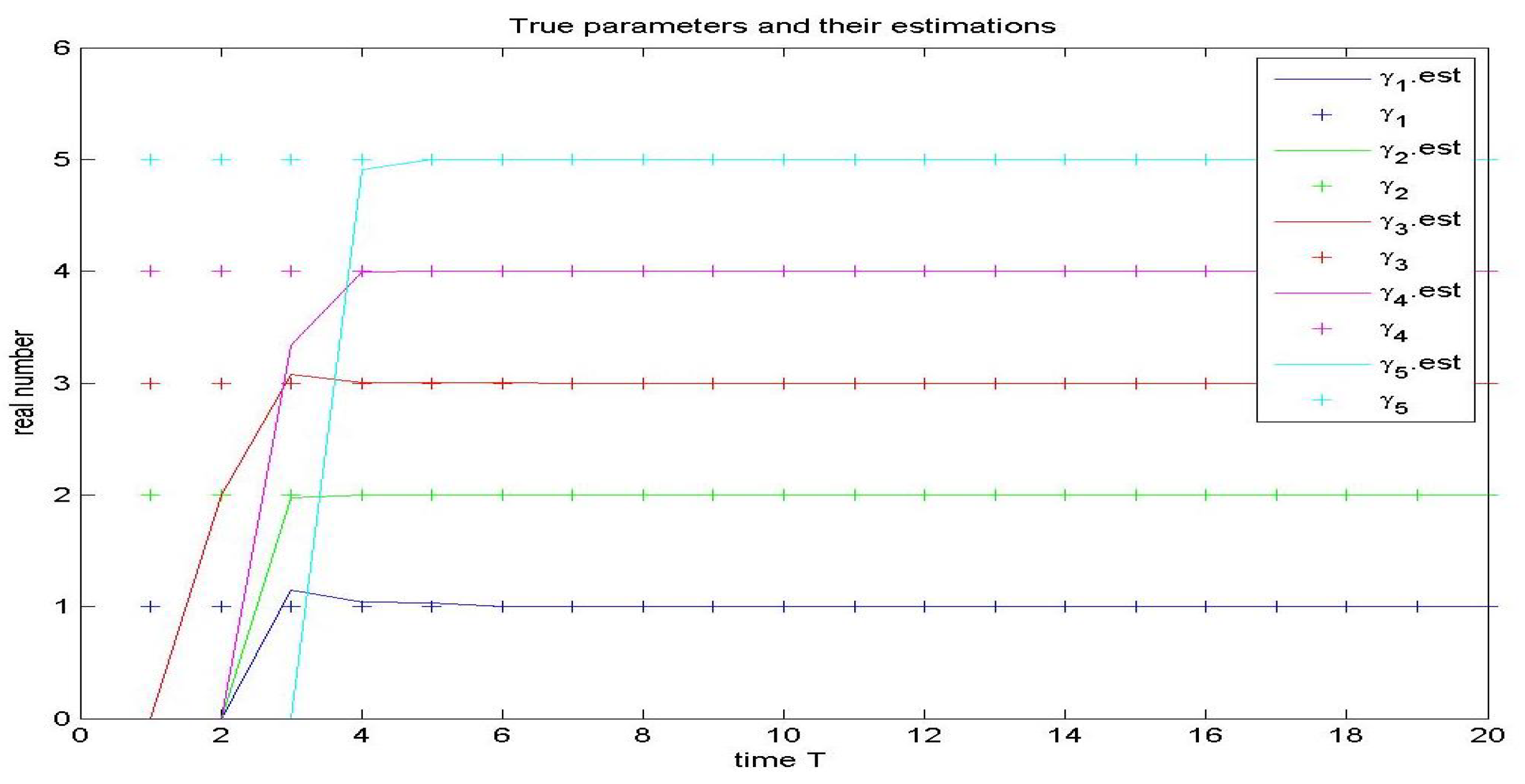
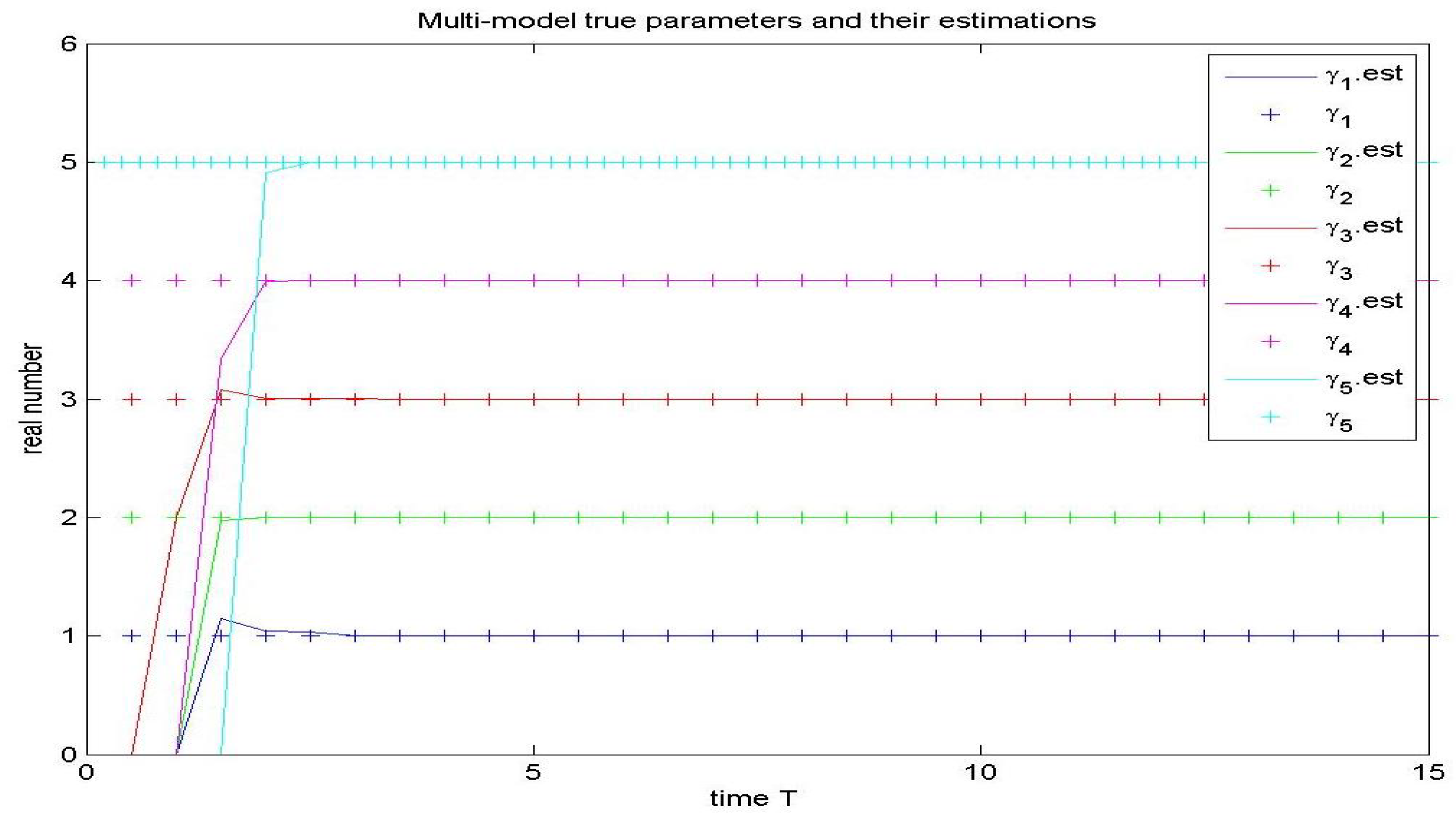
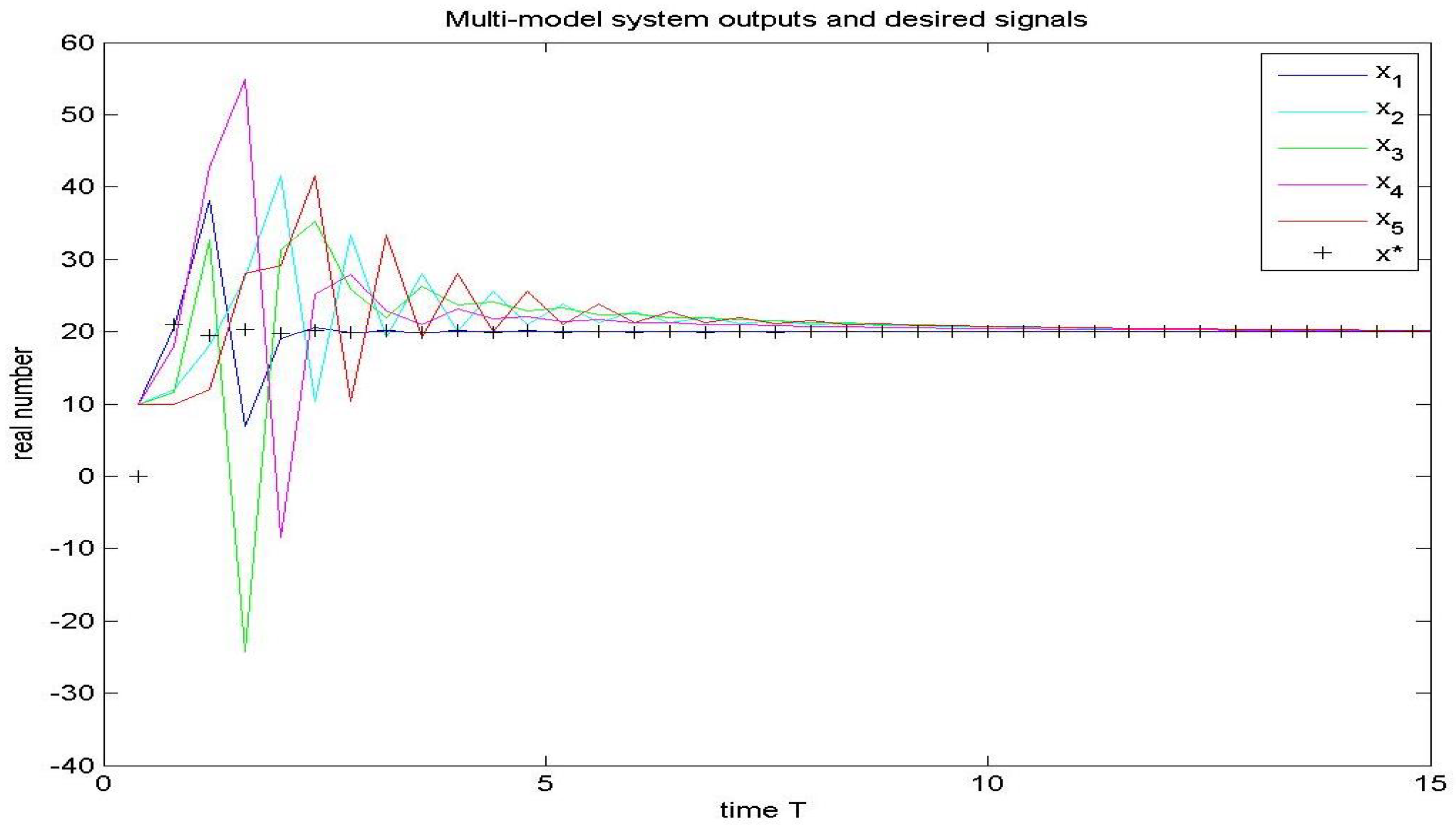
7. Simulations

To test and verify the feasibility and effectiveness of the theoretical results, we consider a non-linear discrete-time coupled MAS consisting of five agents. The dynamics model of agent i is

$$\begin{array}{c}\hfill x_i(T+1)=g_i({\gamma }_i,x_i\left(T\right),{\psi }_i\left(T\right))+u_i\left(T\right),\end{array}$$

(43)

where

$$\left\{\begin{array}{cc}\hfill g_1\left(T\right)& ={\gamma }_1^2{x}_1\left(T\right)+{\gamma }_1{x}_4\left(T\right)+sin{\gamma }_1{x}_4\left(T\right))\hfill \\ \hfill g_2\left(T\right)& ={\gamma }_2{x}_2\left(T\right)+{\gamma }_2^2{e}^{-\left|x_3\left(T\right)\right|}+cos\left({\gamma }_2{x}_5\left(T\right)\right)\hfill \\ \hfill g_3\left(T\right)& =({\gamma }_3^3-5{\gamma }_3-3)x_3\left(T\right)+cos\left({\gamma }_3{x}_1\left(T\right)\right)+{\gamma }_3{e}^{-\left|x_4\left(T\right)\right|}\hfill \\ \hfill g_4\left(T\right)& =x_4\left(T\right)+{\gamma }_4^{2}cos\left(x_2\left(T\right)\right)\hfill \\ \hfill g_5\left(T\right)& ={\gamma }_5{x}_5\left(T\right)+sin\left(x_3\left(T\right)\right)+cos\left(x_2\left(T\right)\right).\hfill \end{array}\right.$$

It follows from (43) that the adjacency matrix is

$$\mathrm{A}=\left[\begin{array}{ccccc}0& 0& 0& 1& 0\\ 0& 0& 1& 0& 1\\ 1& 0& 0& 1& 0\\ 0& 1& 0& 0& 0\\ 0& 1& 1& 0& 0\end{array}\right].$$

(44)

Firstly, by Definition 1 and the adjacency matrix, we can infer this adjacency matrix is strongly connected. It is clear that Assumption 1 holds. Secondly, the hidden leader (first) agent knows the desired signal, while the other agents are not aware of the desired signal nor the existence of the leader agent, and thus, Assumption 2 holds. Thirdly, give the desired signal $x^{\ast }\left(1\right)=21,x^{\ast }(T+1)=20+\frac{{(-1)}^{T+1}}{T}$ as the reference signal. It is easy to check that, Assumption 3 holds, too. Lastly, it is easy to obtain that Assumption 4 holds.

According to the discussion in Section 4, the distributed controllers are designed as

$$\left\{\begin{array}{c}{u}_1\left(T\right)=-{\widehat{\gamma }}_1^2\left(T\right)x_1\left(T\right)-{\widehat{\gamma }}_1{x}_4\left(T\right)-sin{\widehat{\gamma }}_1\left(T\right)x_4\left(T\right))+x^{\ast }(T+1)\hfill \\ u_2\left(T\right)=-{\widehat{\gamma }}_2{x}_2\left(T\right)-{\widehat{\gamma }}_2^2{\chi }^{-\left|x_3\left(T\right)\right|}-cos\left({\widehat{\gamma }}_{2}x5\left(T\right)\right)+\frac{1}{2}(x_3\left(T\right)+x_5\left(T\right))\hfill \\ u_3\left(T\right)=-({\widehat{\gamma }}_3^3-5{\widehat{\gamma }}_3-3)x_3\left(T\right)-cos\left({\widehat{\gamma }}_3{x}_1\left(T\right)\right)-{\widehat{\gamma }}_3{\chi }^{-\left|x_4\left(T\right)\right|}+\frac{1}{2}(x_1\left(T\right)+x_4\left(T\right))\hfill \\ u_4\left(T\right)=-x_4\left(T\right)-{\widehat{\gamma }}_4^{2}cos\left(x_2\left(T\right)\right)+x_2\left(T\right)\hfill \\ u_5\left(T\right)=-{\widehat{\gamma }}_5{x}_5\left(T\right)-sin\left(x_3\left(T\right)\right)-cos\left(x_2\left(T\right)\right)+\frac{1}{2}(x_2\left(T\right)+x_3\left(T\right)),\hfill \end{array}\right.$$

where ${\widehat{\gamma }}_i$ is the estimate calculated by (4).

$$\left\{\begin{array}{cc}\hfill {\gamma }_1& =1\hfill \\ \hfill {\gamma }_2& =2\hfill \\ \hfill {\gamma }_3& =3\hfill \\ \hfill {\gamma }_4& =4\hfill \\ \hfill {\gamma }_5& =5\hfill \end{array}\right.$$

with the set ${[1,1,1,1,1]}^T$ and $T=0.01$ as the initial outputs, ${[0,0,0,0,0]}^{\prime }$ as the initial parameter estimates, and $w_1=0.7,w_2=0.6,w_3=0.5,w_4=0.4,w_5=0.3$ as the punishment factors.

According to the normal parameter update laws discussed in Section 3.1, the unknown parameters are estimated. Each parameter’s estimate and true value are shown in Figure 1. It can be clearly obtained that, for each agent, each parameter estimate tends to the corresponding true parameter value.

It is easy to see from Figure 2 that the velocity of the hidden leader (first) agent tracking the desired signal is faster than the velocity of the followers because the hidden leader tracks the reference directly and the closed-loop system achieves strong synchronization in the sense of the mean in the presence of strong couplings.

According to the adaptive optimal parameter update laws discussed in Section 3.3, the unknown parameters are estimated. As we can see, for each agent, the parameter estimate tends to converge toward the true parameter value. A comparison of Figure 1 and Figure 3, shows that the multi-model method has advantages of accurate estimation and fast convergence. It is not difficult to see from Figure 2 and Figure 4 that the vibration time and overshoot of each agent output are reduced by multi-model adaptive control. The multi-model adaptive control algorithm is effective in improving the control performance when compared with the normal projection algorithm, based on the simulation results.

8. Conclusions

We investigated a class of distributed multi-model adaptive tracking control for discrete-time coupled MASs. The model of each agent involves non-linearly parameterized dynamics with an unknown parameter and can interact with its neighbors’ information.

To identify the system, we adopted the multi-model method.

Each optimal parameter estimate is chosen from one switching set of its own parameter estimates, which contains the parameter estimate that is obtained by the projection algorithm. Under the multi-model estimate update laws and based on the certainty equivalence principle, the leader agent’s control law is designed using the given desired reference signal, and each follower agent’s local control law is designed relying on the neighbors’ history information. With the distributed adaptive control laws, the desired reference signal is tracked by the hidden leader agent, which is followed by the follower agents. Finally, all the agents track the desired reference signal, and the whole system achieves strong synchronization in the sense of the mean.

Finally, simulations show that the adaptive control method with a switching set of the parameter estimates is effective in improving the control performance. The adaptive control scheme for time-varying strong coupling MASs was discussed.

It is very challenging to design the distributed laws such that the whole system achieves strong synchronization in the sense of the mean in the face of time-varying strong couplings.

References

- Zhang, J.L.; Yan, J.G.; Lv, M.L.; Kong, X.J.; Zhang, P. UAV Formation Flight Cooperative Tracking Controller Design. In Proceedings of the International Conference on Control, Automation, Robotics and Vision, Singapore, 18–21 November 2018. [Google Scholar]
- Zhang, J.L.; Xiao, B.; Lv, M.L.; Zhang, Q. Design and Flight-Stability Analysis of a Closed Fixed-Wing Unmanned Aerial Vehicle Formation Controller. Proc. Inst. Mech. Eng. 2019, 233, 1045–1054. [Google Scholar] [CrossRef]
- Liu, Z.Y.; Li, Y.Z.; Wu, Y.Q.; He, S.H. Formation Control of Nonholonomic Unmanned Ground Vehicles via Unscented Kalman Filter-based Sensor Fusion Approach. ISA Trans. 2022, 125, 60–71. [Google Scholar] [CrossRef] [PubMed]
- Hwang, C.L.; Chang, N.W. Fuzzy Decentralized Sliding-Mode Control of a Car-Like Mobile Robot in Distributed Sensor-Network Spaces. IEEE Trans. Fuzzy Syst. 2008, 16, 97–109. [Google Scholar] [CrossRef]
- Zhao, Y.; Guo, G. Distributed Tracking Control of Mobile Sensor Networks with Intermittent Communications. J. Frankl. Inst. 2017, 354, 3634–3647. [Google Scholar] [CrossRef]
- Meng, M.; Xiao, G.X.; Li, B.B. Adaptive Consensus for Heterogeneous Multi-Agent Systems Under Sensor and Actuator Attacks. Automatica 2020, 122, 109242. [Google Scholar] [CrossRef]
- Rouzegar, H.; Khosravi, A.; Sarhadi, P. Spacecraft Formation Flying Control Around L2 Sun-Earth Libration Point Using On-Off SDRE Approach. Adv. Space Res. 2021, 67, 2172–2184. [Google Scholar] [CrossRef]
- Gao, Z.F.; Wang, S. Fault Estimation and Fault Tolerance Control for Spacecraft Formation Systems with Actuator Fault and Saturation. Optim. Control Appl. Methods 2021, 42, 1591–1611. [Google Scholar] [CrossRef]
- Ma, X.P.; Yang, P.L.; Dong, H.Y.; Yang, J.; Yao, Z. Secondary Control Strategy of Islanded Micro-grid Based on Multi-agent Consistency. In Proceedings of the IEEE Conference on Energy Internet and Energy System Integration, Beijing, China, 26–28 November 2017. [Google Scholar]
- Chen, X. Multimode Coordination Control Method for Microgrid Cluster Based on Adaptive Power Control and Routing Algorithm. J. Nanoelectron. Optoelectron. 2022, 17, 72–81. [Google Scholar] [CrossRef]
- Zhao, Y.J.; Liu, C.G.; Liu, X.P.; Wang, H.Q.; Zhou, Y.C. Adaptive Tracking Control for Stochastic Nonlinear Systems with Unknown Virtual Control Coefficients. Int. J. Robust Nonlinear Control 2022, 32, 1331–1354. [Google Scholar] [CrossRef]
- Yan, C.H.; Zhang, W.; Guo, H.; Zhu, F.L.; Qian, Y.C. Distributed Adaptive Time-Varying Formation Control for Lipschitz Nonlinear Multi-agent Systems. Trans. Inst. Meas. Control 2022, 44, 272–285. [Google Scholar] [CrossRef]
- Wang, X.M.; Sun, J.S.; Wu, Z.X.; Li, Z.T. Robust Integral of Sign of Error-Based Distributed Flocking Control of Double-Integrator Multi-Agent Systems with a Varying Virtual Leader. Int. J. Robust Nonlinear Control 2022, 32, 286–303. [Google Scholar] [CrossRef]
- Hu, W.; Wen, G.G.; Rahmani, A.; Yang, G.Y. Distributed Consensus Tracking of Unknown Nonlinear Chaotic Delayed Fractional-order Multi-Agent Systems with External Disturbances Based on ABC Algorithm. Commun. Nonlinear Sci. Numer. Simul. 2019, 71, 101–117. [Google Scholar] [CrossRef]
- Li, J.; Li, H.; Zhang, Z.H.; Li, X.B.; Yang, X.L. Event-Triggered Adaptive NN Tracking Control with Dynamic Gain for a Class of Unknown Nonlinear Systems. Neurocomputing 2022, 467, 292–299. [Google Scholar] [CrossRef]
- Bian, Y.G.; Zhang, J.J.; Hu, Q.J.; Ding, R.J. Self-Triggered Distributed Model Predictive Control for Cooperative Diving of Multi-AUV System. Ocean Eng. 2023, 267, 113262. [Google Scholar] [CrossRef]
- Distributed Pinning Controllers Design for Set Stabilization of k-Valued Logical Control Networks. Math. Model. Control 2023, 3, 61–72. [CrossRef]
- Davis, J.H.; Dryden, G.H. Centralized Traffic Control and Train Control of the Baltimore and Ohio Railroad. Trans. Am. Inst. Electr. Eng. 2009, 52, 308–312. [Google Scholar] [CrossRef]
- Narmanlioglu, O.; Uysal, M. Event-Triggered Adaptive Handover for Centralized Hybrid VLC/MMW Networks. IEEE Trans. Commun. 2022, 70, 455–468. [Google Scholar] [CrossRef]
- Hui, Y.; Xia, X.H. Adaptive Leaderless Consensus of Agents in Jointly Connected Networks. Neurocomputing 2017, 241, 64–70. [Google Scholar] [CrossRef]
- Chen, C.; Lewis, F.L.; Li, X.L. Event-Triggered Coordination of Multi-Agent Systems via a Lyapunov-Based Approach for Leaderless Consensus. Automatica 2022, 136, 109936. [Google Scholar] [CrossRef]
- Liu, W.; Huang, J. Adaptive Leader-Following Consensus for a Class of Higher-order Nonlinear Multi-Agent Systems with Directed Switching Networks. Automatica 2017, 79, 84–92. [Google Scholar] [CrossRef]
- Zhao, M.J.; Peng, Y.; Wang, Y.Y.; Zhang, D.; Luo, J.; Pu, H.Y. Concise Leader-follower Formation Control of Under Actuated Unmanned Surface Vehicle with Output Error Constraints. Trans. Inst. Meas. Control 2022, 44, 1081–1094. [Google Scholar] [CrossRef]
- Zhang, P.; Xue, H.F.; Gao, S.; Zhang, J.L. Distributed Adaptive Consensus Tracking Control for Multi-Agent System with Communication Constraints. IEEE Trans. Parallel Distrib. Syst. 2021, 32, 1293–1306. [Google Scholar] [CrossRef]
- Yang, R.H.; Zhou, D.Y. Distributed Event-Triggered Tracking Control of Heterogeneous Discrete-Time Multi-Agent Systems with Unknown Parameters. J. Syst. Sci. Complex. 2022, 35, 1330–1347. [Google Scholar] [CrossRef]
- Lu, Y.R.; Liao, F.C.; Liu, H.Y.; Usman. Cooperative Preview Tracking Problem of Discrete-Time Linear Multi-Agent Systems: A Distributed Output Regulation Approach. ISA Trans. 2019, 85, 33–48. [Google Scholar] [CrossRef] [PubMed]
- Liu, C.; Jiang, B.; Wang, X.F.; Yang, H.L.; Xie, S.R. Distributed Fault-Tolerant Consensus Tracking of Multi-Agent Systems Under Cyber-Attacks. IEEE/CAA J. Autom. Sin. 2022, 9, 1037–1048. [Google Scholar] [CrossRef]
- Li, X.; Wang, L.L.; Zhang, Y.S. Distributed Continuous-Time Containment Control of Heterogeneous Multiagent Systems with Nonconvex Control Input Constraints. Complexity 2022, 2022, 7081091. [Google Scholar] [CrossRef]
- Hamdan, T.B.; Mercere, G.; Dairay, T.; Meunier, R.; Tremblay, P.; Coirault, P. Tracking Distributed Parameters System Dynamics with Recursive Dynamic Mode Decomposition with Control. SIAM J. Appl. Dyn. Syst. 2023, 22, 37–64. [Google Scholar] [CrossRef]
- Wen, N.Q.; Wu, A.G.; Dong, R.Q. Distributed Adaptive Neural Network Fixed-Time Leader-Follower Attitude Consensus Control for Multiple Rigid Spacecraft. Int. J. Adapt. Control Signal Process. 2023, 37, 553–582. [Google Scholar] [CrossRef]
- Lainiotis, D.G. Optimal Adaptive Estimation: Structure and Parameter Adaption. IEEE Trans. Autom. Control 1971, 16, 160–170. [Google Scholar] [CrossRef]
- Middleton, R.H.; Goodwin, G.C.; Hill, D.J.; Mayne, D.Q. Design Issues in Adaptive Control. IEEE Trans. Autom. Control 1988, 33, 50–58. [Google Scholar] [CrossRef]
- Zhivoglyadov, P.V.; Middleton, R.H.; Fu, M. Localization Based Switching Adaptive Control for Time-Varying Discrete-Time Systems. IEEE Trans. Autom. Control 2000, 45, 752–755. [Google Scholar] [CrossRef]
- Zhang, Y.J.; Chai, T.Y.; Wang, H.; Fu, J.; Zhang, L.Y.; Wang, Y.G. An Adaptive Generalized Predictive Control Method for Nonlinear Systems Based on ANFIS and Multiple Models. IEEE Trans. Fuzzy Syst. 2010, 18, 1070–1082. [Google Scholar] [CrossRef]
- Narendra, K.S.; Xiang, C. Adaptive Control of Discrete-Time Systems Using Multiple Models. IEEE Trans. Autom. Control 2000, 45, 1669–1686. [Google Scholar] [CrossRef]
- Zhai, J.Y.; Fei, S.M. Multiple Models Adaptive Control Based on Online Optimization. Syst. Eng. Electron. 2009, 31, 2185–2188. [Google Scholar]
- Yue, F.; Chai, T.Y. Nonlinear Multivariable Adaptive Control Using Multiple Models and Neural Networks. Automatica 2007, 43, 1101–1110. [Google Scholar] [CrossRef]
- Miao, H.; Wang, X.; Wang, Z.L.; Feng, Q. Multiple Models Adaptive Control Based on Cluster-optimization for a Class of Nonlinear System. In Proceedings of the Intelligent Control and Automation, Beijing, China, 6–8 July 2011. [Google Scholar] [CrossRef]
- Niu, Y.G.; Li, X.M.; Lin, Z.W.; Li, M.Y. Multiple Models Decentralized Coordinated Control of Doubly Fed Induction Generator. Int. J. Electr. Power Energy Syst. 2015, 64, 921–930. [Google Scholar] [CrossRef]
- Zhang, X.H.; Chang, Z.Y.; Wang, Y.H. Multi-Model Method Decentralized Adaptive Control for a Class of Discrete-Time Multi-Agent Systems. IEEE Access 2020, 8, 193717–193727. [Google Scholar] [CrossRef]
- Zhang, X.H.; Ma, H.B.; Yang, C.G. Decentralised Adaptive Control of a Class of Hidden Leader-follower Non-linearly Parameterised Coupled MASs. IET Control Theory Appl. 2017, 11, 3016–3025. [Google Scholar] [CrossRef]
- Ge, S.S.; Yang, C.G.; Li, Y.N.; Tong, H.L. Decentralized Adaptive Control of a Class of Discrete-time Multi-agent Systems for Hidden Leader Following Problem. In Proceedings of the IEEE/RSJ International Conference on Intelligent Robots and Systems, St. Louis, MO, USA, 10–15 October 2009. [Google Scholar] [CrossRef]
- Zhang, X.H.; Ma, H.B.; Wang, J.N. Decentralized Adaptive Control of a Class of Discrete-Time Nonlinear Hidden-Leader Follower Multi-Agent Systems. In Proceedings of the 2017 36th Chinese Control Conference (CCC), Dalian, China, 26–28 July 2017. [Google Scholar]
Disclaimer/Publisher’s Note: The statements, opinions and data contained in all publications are solely those of the individual author(s) and contributor(s) and not of MDPI and/or the editor(s). MDPI and/or the editor(s) disclaim responsibility for any injury to people or property resulting from any ideas, methods, instructions or products referred to in the content. |
© 2024 by the authors. Licensee MDPI, Basel, Switzerland. This article is an open access article distributed under the terms and conditions of the Creative Commons Attribution (CC BY) license (https://creativecommons.org/licenses/by/4.0/).
Share and Cite
Yang, J.; Lee, B.G. Distributed Adaptive Tracking Control of Hidden Leader-Follower Multi-Agent Systems with Unknown Parameters. Mathematics 2024, 12, 1013. https://doi.org/10.3390/math12071013
Yang J, Lee BG. Distributed Adaptive Tracking Control of Hidden Leader-Follower Multi-Agent Systems with Unknown Parameters. Mathematics. 2024; 12(7):1013. https://doi.org/10.3390/math12071013
Chicago/Turabian StyleYang, Jie, and Byung Gook Lee. 2024. "Distributed Adaptive Tracking Control of Hidden Leader-Follower Multi-Agent Systems with Unknown Parameters" Mathematics 12, no. 7: 1013. https://doi.org/10.3390/math12071013