Efficient Maintenance of Minimum Spanning Trees in Dynamic Weighted Undirected Graphs

Abstract

This paper presents an algorithm for effectively maintaining the minimum spanning tree in dynamic weighted undirected graphs. The algorithm efficiently updates the minimum spanning tree when the underlying graph structure changes. By identifying the portion of the original tree that can be preserved in the updated tree, our algorithm avoids recalculating the minimum spanning tree from scratch. We provide proof of correctness for the proposed algorithm and analyze its time complexity. In general scenarios, the time complexity of our algorithm is comparable to that of Kruskal’s algorithm. However, the experimental results demonstrate that our algorithm outperforms the approach of recomputing the minimum spanning tree by using Kruskal’s algorithm, especially in medium- and large-scale dynamic graphs where the graph undergoes iterative changes.

1. Introduction

Given a weighted undirected connected graph, the minimum spanning tree (MST) problem involves finding a subgraph spanning all vertices in the graph without ring structures and with the minimized sum of edge weights. This problem was first introduced by Brouvka in 1926. Nesetril and Nesetrilova [1] have provided a detailed overview of the origin and development of the MST problem. MST has widespread applications in real-life scenarios, including transportation problems, communication network design, and many other combinatorial optimization problems. For example, MST is commonly employed in clustering (see [2,3,4]). It is a common method to study relationships in financial markets by constructing an MST from correlation matrices (see [5,6,7]). MST is also used for analyzing brain networks (see [8,9,10]). The MST problem is also common in various production and life applications, such as power grid configuration [11], dynamic power distribution reconfiguration [12], optimal configuration problem [13], etc.

Real-world problems requiring solutions to the MST problem often involve graphs of immense scale and dynamic changes. Although polynomial-time algorithms exist for the MST problem, the real-time computation for large-scale graphs remains challenging. Moreover, real-world scenarios typically involve modifications to only a small portion of the original graph. Recalculating the entire graph using MST algorithms for the new graph results in significant redundant computations. This underscores the need for effective maintenance of the MST in dynamic graphs. Solutions designed for static problems are generally inadequate to meet the requirements of dynamic graphs [14]. In the context of the Internet of Things (IoT) domain, Wireless Ad Hoc Networks are commonly used and often employ a minimum dominating tree (MDT) structure as the backbone for network traffic management [15]. MDT is a spanning tree that encompasses a specific dominating set within the network. Given the dynamic nature of Ad Hoc Networks, they frequently change over time, necessitating corresponding adjustments in their backbone structure. To ensure efficient maintenance of the backbone, an effective solution to the dynamic minimum spanning tree (MST) problem is necessary. Moreover, the algorithm for dynamic MST can also be employed as a sub-procedure in the MDT algorithm to enhance convergence [16].

This paper studies the problem of updating the original MST of a graph when its structure changes. Given a weighted undirected graph and its MST, the problem queries a new MST based on the original one if the graph changes its structure, i.e., if  edges and vertices are added or removed.

Existing algorithms for maintaining the minimum spanning tree in dynamic graphs are usually designed for various scenarios. Frederickson et al. [17] proposed a top-tree-based algorithm, which is specifically designed for graphs where the maximum degree of vertices is three. Amato et al. [18] conducted the first experimental study on dynamic minimum spanning tree algorithms. They implemented different versions of Frederickson’s algorithm using partitioning and top-trees. Additionally, to achieve the fastest random input, Henzinger and King [19] introduced a fully dynamic minimum spanning tree algorithm. Holm et al. [20] improved the algorithm proposed by Henzinger and King. They were the first to introduce a fully dynamic minimum spanning tree algorithm with logarithmic-time complexity. Cattaneo et al. [21] further optimized several algorithms for this problem. Eppstein et al. [22] introduced sparsification techniques on top of Frederickson’s algorithm, reducing the time complexity to $O\left(\sqrt{n}\right)$. Based on Eppstein’s work, Kopelowitz et al. [23] proposed the algorithm with the best-known results, achieving a time complexity of $O(\sqrt{n}·lgn)$ per update for each vertex, but only allowing single-edge updates. Tarjan and Wereck [24] conducted experiments on two variants of dynamic tree data structures (self-adjusting and worst-case) and compared their advantages and disadvantages. Chen et al. [25] proposed the LDP-MST algorithm, which calculates density based on the results of the natural neighbor search algorithm, identifies local density peaks, and then constructs the minimum spanning tree. Junior et al. [26] proposed an algorithm for solving the variant of the fully dynamic minimum spanning tree problem, addressing the incremental minimum spanning tree problem through complete backtracking. Anderson et al. [22] proposed a parallel batch-processing dynamic algorithm for incremental minimum spanning trees. They introduced a parallel data structure for batch-processing incremental MSF problems, achieving polynomial time for each edge insertion, which is more efficient than the fastest sequential single-update data structure for sufficiently large batches. Tseng et al. [27] implemented parallelization based on Holm et al.’s work and proposed a parallel batch algorithm to maintain MSF.

After reviewing the current state of research, it is apparent that the majority of the existing studies have predominantly concentrated on scenarios involving single changes. In this paper, our objective is to explore a specific scenario where a portion of the graph undergoes alteration. Furthermore, we propose a method that is well suited for preserving MST in situations where the graph undergoes iterative structural modifications, with only a small segment of the graph being altered in each iteration.

The following of the paper is organized as follows: Section 2 describes the problem studied by this paper in detail; Section 3 introduces the proposed MST maintenance algorithm; Section 4 includes theoretical proofs and an analysis of the time complexity of the proposed algorithm; Section 5 presents the experiments conducted and evaluates the proposed algorithm; finally, Section 6 concludes the paper and outlines prospects for future work.

2. Problem Description

Given a weighted undirected graph $G=(V,E)$, where V is the set of vertices and E is the set of edges, and its minimum spanning tree, this paper investigates a rapid updating and generation algorithm for the new minimum spanning tree when partial structural changes occur in graph G. If the updated graph becomes a non-connected graph, the algorithm should provide a minimum spanning forest. This section describes two specific scenarios of graph changes and generalizes the common variations in the graph accordingly.

2.1. Minimum Spanning Tree of the Subgraph in the Original Graph

If the changes to the graph only involve the removal from the original graph, the updated graph is a subgraph of the original. The problem then becomes finding the minimum spanning tree of a subgraph of the original graph. This is defined as follows: Given a weighted undirected graph $G=(V,E)$ and its spanning tree T, the task is to find the minimum spanning tree $T^{-}$ of graph $G^{-}=(V,E^{-})$, where $E^{-}\subseteq E$.

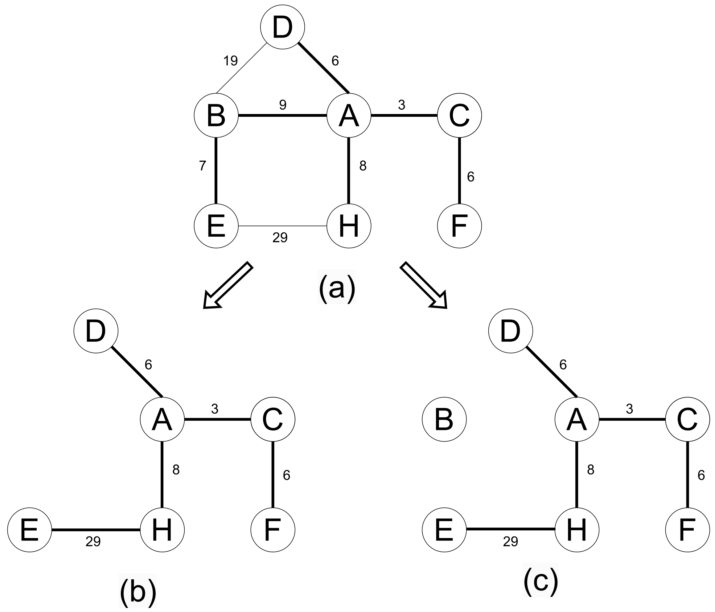
The MST of a subgraph may differ from or be identical to the MST of the original graph. Figure 1 illustrates an example of the subgraph MST problem. Given the original graph shown in Figure 1a, where solid lines represent edges in the MST (following schematic figures), a subgraph is formed by removing edge $⟨A,B⟩$, as depicted in Figure 1b. It can be observed that the MST of this subgraph is different from that of the original graph. If the removed edge is not part of the original MST, the MST of the subgraph is identical to the original MST, as shown in Figure 1c.

Figure 1. Illustration of subgraph minimum spanning tree problem. (a) The original graph and its MST; (b) Removing $⟨A,B⟩$ changes the MST; (c) Removing $⟨H,E⟩$ does not change the MST. (Numbers on edges represent the edge weights. The following figures are the same).

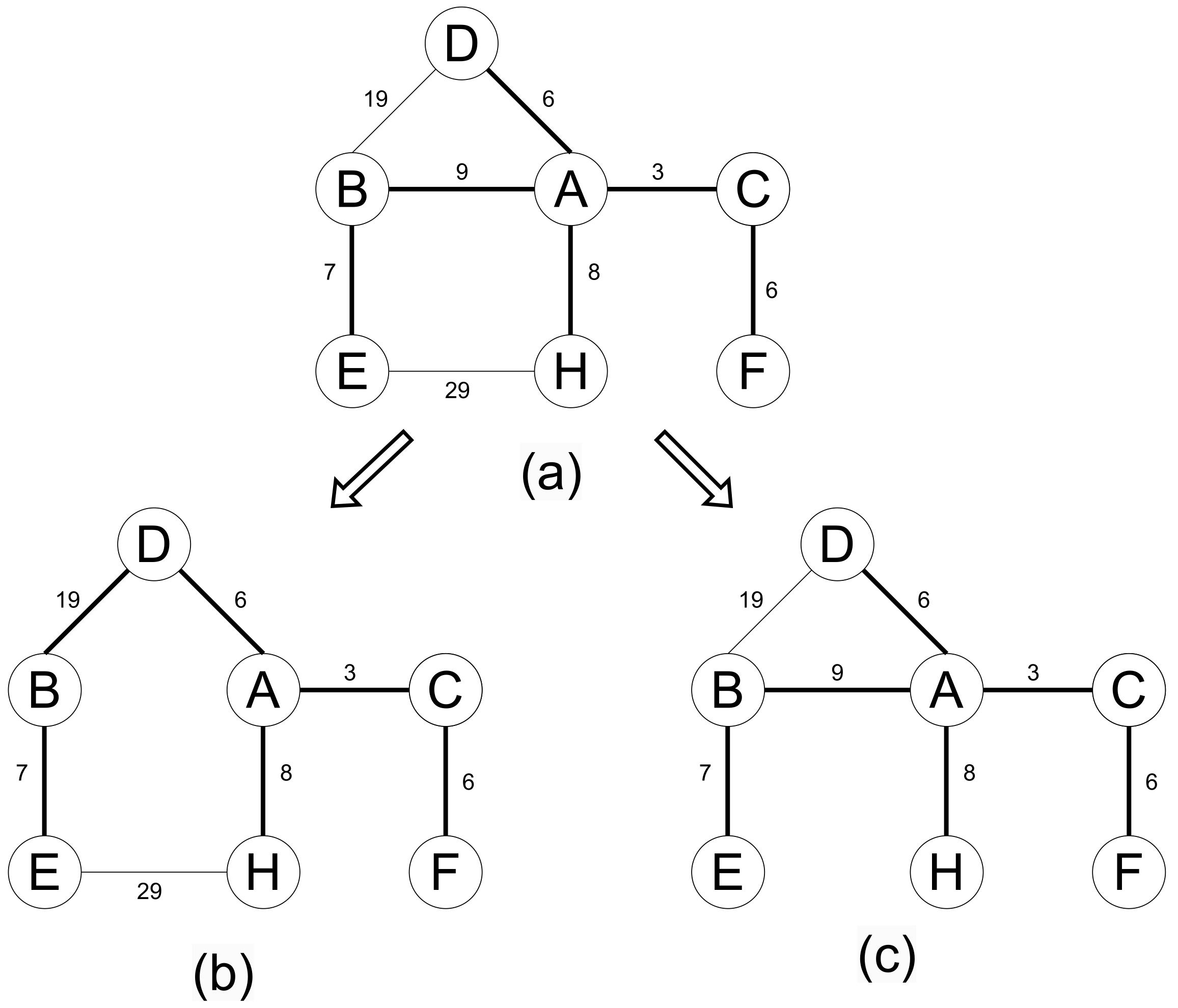
Removing a vertex from the original graph can be reduced to removing multiple edges. The new minimum spanning tree obtained after removing a vertex from the original graph has the same weight as the minimum spanning forest obtained by removing all edges connected to this vertex, after which this vertex becomes an isolated vertex, and its presence or absence does not affect the weight of the minimum spanning tree. For example, in the original graph shown in Figure 2a, after deleting vertex B, the subgraph and its minimum spanning tree are shown in Figure 2b. After deleting all edges connected to vertex B, the subgraph and its minimum spanning forest are shown in Figure 2c. Deleting a vertex from the original graph changes the minimum spanning tree.

Figure 2. Deleting vertex B provides the same MST as deleting all edges related to B. (a) The original graph; (b) Deleting vertex B; (c) Deleting all edges connected to vertex B.

2.2. Minimum Spanning Tree of the Supergraph in the Original Graph

If the modifications to the graph only involve additions to the original graph, then the updated graph becomes a supergraph of the original. The problem becomes finding the minimum spanning tree (MST) of a certain supergraph of the original graph. The definition is as follows: Given a weighted undirected graph $G=(V,E)$ and its spanning tree T, the objective is to find the minimum spanning tree $T^{+}$ of graph $G^{+}=(V,E^{+})$, where $E^{+}\subset E$.

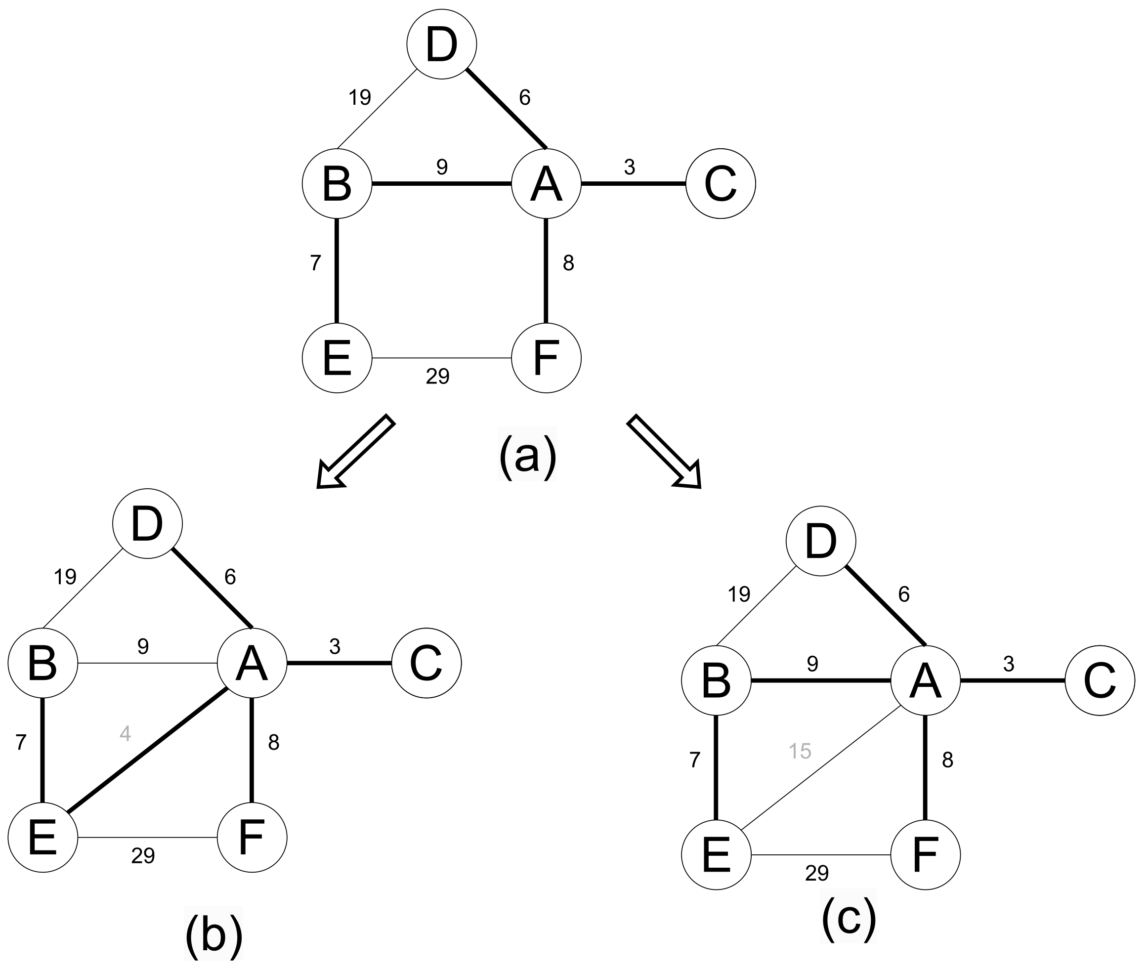
Figure 3 illustrates an example of the supergraph minimum spanning tree problem. Given the original graph and its spanning tree shown in Figure 3a, the supergraph with the added edge $⟨A,E⟩$ and its minimum spanning tree are depicted in Figure 3b. It can be observed that in this example, the spanning tree of the supergraph differs from that of the original graph. Through analysis, it can be deduced that when the weight of the added edge is less than the weight of a certain edge forming a cycle in the original MST, the new MST changes. For example, in this instance, adding $⟨A,E⟩$ creates a cycle in the original MST: $⟨A,E⟩$ — $⟨A,B⟩$ — $⟨B,E⟩$; the weight of $⟨A,E⟩$ is less than the weight of $⟨A,B⟩$ in the cycle. If the weight of the added edge is greater than the weights of all other edges in the cycle, then the MST of the supergraph remains the same as that of the original graph, as shown in Figure 3c.

Figure 3. Example of a supergraph minimum spanning tree. (a) The original graph and its MST; (b) Adding edge $⟨Q,C⟩$ with weight 4 changes the MST; (c) Adding edge $⟨Q,C⟩$ with weight 15 does not change the MST.

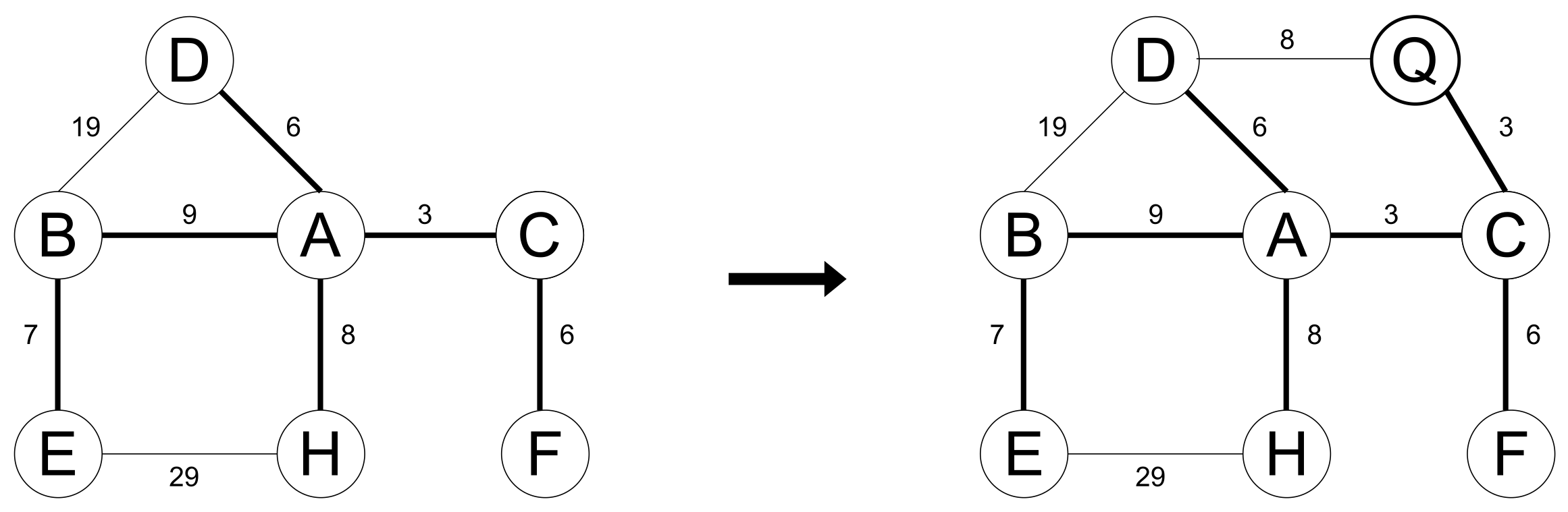
From the original graph, the addition of a vertex can be reduced to adding multiple edges. Consider the vertex to be added firstly as an isolated vertex in the original graph, and then add the edges associated with it to the original graph. For example, considering the original graph and its spanning tree shown in Figure 4 (left), after adding vertex Q along with edges $⟨Q,C⟩$ and $⟨Q,D⟩$, the resulting supergraph and its minimum spanning tree are illustrated in Figure 4 (right). Adding a non-isolated vertex to the original graph inevitably alters the minimum spanning tree.

Figure 4. Example of a supergraph with added vertex Q.

2.3. Minimum Spanning Tree after Modifications to Original Graph

When the modified graph is not a subgraph or supergraph of the original graph, the transformation can be broken down into two distinct sub-processes: removing edges and adding new edges. This leads to the transformation of the original problem into two processes, solving a subgraph minimum spanning tree and a supergraph minimum spanning tree.

Let the original graph be denoted by $G=(V,E)$ and the changed graph by $G^{\prime }=(V,E^{\prime })$. First, we determine the set of edges removed in $G^{\prime }$ compared with G as $E^{-}=E\setminus E^{\prime }$ and the set of edges added in $G^{\prime }$ compared with G as $E^{+}=E^{\prime }\setminus E$. Subsequently, we calculate the minimum spanning tree of subgraph $G^{-}=(V,E\setminus E^{-})$. Then, we calculate the minimum spanning tree of supergraph $G^{-+}=(V,E\setminus E^{-}\cup E^{+})$, where $G^{-+}$ is equivalent to $G^{\prime }$.

For example, as depicted in Figure 5a, the original graph transforms into the new graph shown in Figure 5c (by deleting $⟨A,E⟩$ and adding $⟨A,B⟩$). To find the minimum spanning tree of the resulting graph, one can first determine the minimum spanning tree of the subgraph (by deleting $⟨A,E⟩$), as shown in Figure 5b, and then compute the minimum spanning tree of the supergraph (by adding $⟨A,B⟩$), which is equivalent to the graph in Figure 5c.

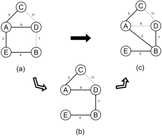
Figure 5. Schematic diagram of the splitting operation to solve the minimum spanning tree of the new graph after the change. (a) The original graph and its MST; (b) Removing $⟨A,E⟩$; (c) Removing $⟨A,E⟩$ and adding $⟨A,B⟩$.

3. Fast Updating and Maintenance Algorithm for Minimum Spanning Trees

This section describes an algorithm for efficiently updating and maintaining the minimum spanning tree in a dynamic graph. To facilitate the subsequent algorithm descriptions, we first define the following symbols:

• $E^0$: ordered set of edges in graph E, where the edges are sorted in ascending order of weight.
• $E^{+}$: set of edges added in the new graph compared with the original graph.
• $E^{-}$: set of edges removed in the new graph compared with the original graph.
• D: array representing the disjoint-set data structure. If $D\left[i\right]>0$, it signifies that vertex i is a non-representative vertex, and $D\left[i\right]$ denotes the representative vertex number of the connected component containing vertex i. If $D\left[i\right]<0$, it indicates that vertex i is the representative vertex of its connected component, and the absolute value of $D\left[i\right]$ is the number of vertices in the current connected component. This data structure is globally visible throughout the algorithm.
• V: visitation array used as an auxiliary data structure for reconstructing the disjoint set during sub-processes. $V\left[i\right]=\mathrm{TRUE}$ indicates that vertex i has been visited; otherwise, $V\left[i\right]=\mathrm{FALSE}$. This data structure is globally visible throughout the algorithm.
• T: set of edges for the current spanning tree.
• $T^{\prime }$: set of edges for the updated spanning tree.

3.1. Framework of the Algorithm

The overall framework of the algorithm is described in Algorithm 1. The input to the algorithm consists of the given graph G, the ordered edge set $E^0$ of G, the minimum spanning tree T of G, the set of edges to be added $E^{+}$, and the set of edges to be removed $E^{-}$. The algorithm first calculates the minimum spanning tree of the subgraph obtained by removing the edges in $E^{-}$ from the original graph (Line 7). Subsequently, it computes the minimum spanning tree of the new graph obtained by adding the edges in $E^{+}$ to this subgraph and its spanning tree (Line 11).

It is worth noting that the algorithm requires information about the sorted edges of the current graph based on edge weights (ordered edge set $E^0$) to enhance computational speed. Upon completion of the algorithm, the ordered edge set $E^{\prime 0}$ of the new graph will be returned for subsequent updates and maintenance of the minimum spanning tree when further changes occur. The updating algorithm for the minimum spanning tree of the subgraph in Algorithm 1, as well as the updating algorithm for the supergraph, will be specifically described in the following sections.

Algorithm 1 MST updating: dynamic graph MST fast updating and maintenance algorithm

1: Input: Graph $G=(V,E)$, an ordered edge set $E^0$, a minimum spanning tree T, sets of edges to be added $E^{+}$ and to be removed $E^{-}$. 2: Output: Updated minimum spanning tree $T^{\prime }$ and modified edge set $E^{\prime 0}$. 3: procedure MST_UPDATE($G,E^0,T,E^{+},E^{-}$) 4:     $T^{\prime }\leftarrow \varnothing$ 5:     if $E^{-}\ne \varnothing$ then 6:         $G\leftarrow$ Remove edges in $E^{-}$ from G. 7:         $T^{\prime }\leftarrow MST\_update\_sub(G,E^0,T,E^{-})$ 8:     end if 9:     if $E^{+}\ne \varnothing$ then 10:         $G\leftarrow$ Add edges in $E^{+}$ to G. 11:         $T^{\prime },E^{\prime 0}\leftarrow MST\_update\_super(G,E^0,T^{\prime },E^{+},E^{-})$ 12:     end if 13:     return $T^{\prime },E^{\prime 0}$ 14: end procedure

3.2. Updating and Maintenance of Minimum Spanning Trees for Subgraphs

This section describes the updating algorithm for the minimum spanning tree of the subgraph, as depicted in Algorithm 2.

Algorithm 2 MST updating subgraph: dynamic graph MST fast updating and maintenance algorithm

1: Input: Graph $G=(V,E)$, ordered edge set $E^0$, minimum spanning tree T, set of edges to be removed $E^{-}$. 2: Output: Updated minimum spanning tree $T^{\prime }$. 3: procedure MST_UPDATE($G,E^0,T,E^{-}$) 4:     $T^{\prime }\leftarrow \mathrm{R}\mathrm{E}\mathrm{M}\mathrm{O}\mathrm{V}\mathrm{E}\_\mathrm{E}\_\mathrm{F}\mathrm{R}\mathrm{O}\mathrm{M}\_\mathrm{T}\mathrm{R}\mathrm{E}\mathrm{E}(T,E^{-})$ 5:     if T’ = T then 6:         return $T^{\prime }$ 7:     end if 8:     $n\leftarrow \mathrm{R}\mathrm{E}\mathrm{B}\mathrm{U}\mathrm{I}\mathrm{L}\mathrm{D}\mathrm{\_}\mathrm{D}\mathrm{I}\mathrm{S}\mathrm{J}\mathrm{O}\mathrm{I}\mathrm{N}\mathrm{T}\_\mathrm{S}\mathrm{E}\mathrm{T}\left(T^{\prime }\right)$ 9:     if $n=1$ then 10:         return $T^{\prime }$ 11:     end if 12:     for $e\in E^0$ do 13:         if $e\notin T^{\prime }$ and $e\notin E^{-}$ then 14:            $T^{\prime }\leftarrow \mathrm{C}\mathrm{H}\mathrm{E}\mathrm{C}\mathrm{K}\mathrm{\_}\mathrm{I}\mathrm{F}\_\mathrm{T}\mathrm{R}\mathrm{E}\mathrm{E}\_\mathrm{E}\mathrm{D}\mathrm{G}\mathrm{E}(T^{\prime },e)$ 15:         end if 16:         if $|T^{\prime }|=|V|-1$ then 17:            return $T^{\prime }$ 18:         end if 19:     end for 20:     return $T^{\prime }$ 21: end procedure

The algorithm takes as input the current graph G, the minimum spanning tree T before the graph changes, the set of deleted edges $E^{-}$, and the ordered set of edges $E^0$ from the original graph. The algorithm first removes $E^{-}$ from the original minimum spanning tree T to obtain the pruned subgraph $T^{\prime }$ (Line 4). Subsequently, the algorithm reconstructs and returns the disjoint set data structure D based on $T^{\prime }$ by using a depth-first traversal process, along with the count (n) of connected components in $T^{\prime }$.

If $T^{\prime }$ equals T or forms a connected structure ($n=1$), then it is the updated minimum spanning tree (Lines 6–8). Otherwise, the algorithm iteratively examines the edges in set $E^0$ that do not belong to $T^{\prime }$ or $E^{-}$, and if an edge connects two different connected components in $T^{\prime }$, it is added to $T^{\prime }$ until $T^{\prime }$ has $\left|V\right|-1$ edges. At this point, $T^{\prime }$ becomes the updated minimum spanning tree (Lines 9–16).

The latter part of the algorithm (Lines 9–16) is essentially similar to Kruskal’s algorithm. The key distinction lies in the fact that Kruskal’s algorithm starts building the minimum spanning tree from scratch, while Algorithm 2 maximizes the utilization of the original graph’s minimum spanning tree. It begins constructing the new graph’s minimum spanning tree from the substructure $T^{\prime }$ derived from the original graph’s minimum spanning tree. To facilitate the continuation of Kruskal’s algorithm based on substructure $T^{\prime }$, a disjoint set structure D matching the current $T^{\prime }$ is required. Algorithms 3 and 4 describe the logical steps for obtaining the corresponding disjoint set D based on input $T^{\prime }$.

Algorithm 3 Rebuilding disjoint set and returning current component count

1: Input: Minimum spanning tree $T^{\prime }$. 2: Output: Component count n. 3: procedure REBUILD_DISJOINT_SET($T^{\prime }$) 4:     Set all elements in D to $-1$ 5:     Set all elements in V to FALSE 6:     $u\leftarrow \mathrm{F}\mathrm{I}\mathrm{N}\mathrm{D}\_\mathrm{U}\mathrm{N}\mathrm{V}\mathrm{I}\mathrm{S}\mathrm{I}\mathrm{T}\mathrm{E}\mathrm{D}($) 7:     $n\leftarrow 0$ 8:     while $u>-1$ do 9:         $n\leftarrow n+1$ 10:         $V\left[u\right]\leftarrow \mathbf{TRUE}$ 11:         $\mathrm{C}\mathrm{O}\mathrm{U}\mathrm{N}\mathrm{T}\_\mathrm{R}\mathrm{E}\mathrm{C}\mathrm{U}\mathrm{R}(T^{\prime },u,u)$ 12:         $u\leftarrow \mathrm{F}\mathrm{I}\mathrm{N}\mathrm{D}\_\mathrm{U}\mathrm{N}\mathrm{V}\mathrm{I}\mathrm{S}\mathrm{I}\mathrm{T}\mathrm{E}\mathrm{D}($) 13:     end while 14:     return n 15: end procedure

Algorithm 4 Recursive sub-procedure for rebuilding the disjoint set

1: Input: Minimum spanning tree $T^{\prime }$, root vertex $v_r$, current vertex v. 2: Output: None. 3: procedure COUNT_RECUR($T^{\prime },v_r,v$) 4:     Reverse $L_v\leftarrow$ Neighbors of vertex v in $T^{\prime }$ 5:     for $u\in L_v$ do 6:         if $V\left[u\right]=\mathbf{FALSE}$ then 7:            $V\left[u\right]\leftarrow \mathbf{TRUE}$ 8:            $D\left[v_r\right]\leftarrow D\left[v_r\right]-1$ 9:            $D\left[u\right]\leftarrow v_r$ 10:            COUNT_RECUR($T^{\prime },v_r,u$) 11:         end if 12:     end for 13: end procedure

Algorithm 3 initializes D and V. It starts by searching for an unvisited vertex in $T^{\prime }$ after initialization (Line 6), marks it as visited, and performs a depth-first traversal starting from it (Line 11). If there are no unvisited vertices after this depth-first traversal, the algorithm terminates; otherwise, it starts over from another unvisited vertex. The sub procedure find_unvisited in Algorithm 3 traverses the vertices in $T^{\prime }$ and returns the index of the first vertex corresponding to a FALSE V value. If all vertices have TRUE V values, find_unvisited returns −1. The detailed logic of the depth-first traversal process count_recur is described in Algorithm 4.

Algorithm 4 is an iterative depth-first traversal operation for a subgraph $T^{\prime }$ to rebuild the disjoint set, with the representative vertex $v_r$ and the current vertex v. If $D\left[v\right]>0$, the value represents the representative of vertex v; if $D\left[v\right]<0$, it indicates that v is a root representative representing all the other vertices in this connected component, and its absolute value represents the number of vertices in the connected component.

Algorithm 5 checks whether the two endpoints of edge e are connected to the two connected components in the current subgraph T. If true, it adds edge e to the current subgraph T, updates the corresponding D values, and returns the updated subgraph $T^{\prime }$. The process of Algorithm 5 is identical to the corresponding steps in Kruskal’s algorithm.

Algorithm 5 Checking if edge e belongs to minimum spanning tree

1: Input: Minimum spanning tree T, edge e. 2: Output: Updated minimum spanning tree $T^{\prime }$. 3: procedure CHECK_IF_TREE_EDGE($T,e$) 4:     $T^{\prime }\leftarrow T$ 5:     $i\leftarrow$ starting vertex of e 6:     $j\leftarrow$ ending vertex of e 7:     while $D\left[i\right]\ge 0$ do 8:         $i\leftarrow D\left[i\right]$ 9:     end while 10:     while $D\left[j\right]\ge 0$ do 11:         $j\leftarrow D\left[j\right]$ 12:     end while 13:     if $i\ne j$ then 14:         if $i<j$ then 15:            $D\left[i\right]\leftarrow D\left[i\right]+D\left[j\right]$ 16:            $D\left[j\right]\leftarrow i$ 17:         else 18:            $D\left[j\right]\leftarrow D\left[i\right]+D\left[j\right]$ 19:            $D\left[i\right]\leftarrow j$ 20:         end if 21:         $T^{\prime }\leftarrow T^{\prime }\cup \left\{e\right\}$ 22:     end if 23:     return $T^{\prime }$ 24: end procedure

This algorithm differs from Kruskal’s algorithm in that it does not compute the spanning tree from scratch but utilizes the original minimum spanning tree of the graph and reconstructs its corresponding disjoint set. The depth-first traversal operation has linear-time complexity, whereas obtaining the same disjoint-set structure using Kruskal’s algorithm involves polynomial-time complexity.

3.3. Updating and Maintenance of Minimum Spanning Trees for Supergraphs

This subsection describes the minimum spanning tree updating algorithm for supergraphs. The algorithmic logic is shown in Algorithm 6. The input of Algorithm 6 includes the current graph G, the minimum spanning tree T before the graph changes, the set of added edges $E^{+}$, the set of deleted edges $E^{-}$, and the ordered set of edges $E^0$ in the original graph. Algorithm 6 first obtains the union of T and $E^{+}$, denoted by $E^{\ast }$; then it executes Kruskal’s algorithm with elements only from $E^{\ast }$; finally, it generates the ordered edge set $E^{\prime 0}$ for the current graph G based on $E^0$, $E^{+}$, and $E^{-}$, which will be used for the subsequent iterations to update the minimum spanning tree. Although a supergraph does not contain any deleted edges compared with the original graph, the deleted edges $E^{-}$ here are the ones from the previous subgraph procedure and are used to generate the ordered edge set $E^{\prime 0}$ for the next iteration.

Algorithm 6 Supergraph minimum spanning tree fast updating and maintenance algorithm

1: Input: Graph G, ordered edge set $E^0$, minimum spanning tree T, set of edges to be added $E^{+}$, set of edges to be removed $E^{-}$. 2: Output: Updated minimum spanning tree $T^{\prime }$, updated ordered edge set $E^{\prime 0}$. 3: procedure MST_UPDATE_SUPER($G,E^0,T,E^{+},E^{-}$) 4:     $E^{\ast }\leftarrow T\cup E^{+}$ 5:     $E^{\ast 0}$: Sort elements in $E^{\ast }$ by weight in ascending order 6:     Set all elements in D to $-1$ 7:     $T^{\prime }\leftarrow \varnothing$ 8:     for $e\in E^{\ast 0}$ do 9:         $T^{\prime }\leftarrow \mathrm{C}\mathrm{H}\mathrm{E}\mathrm{C}\mathrm{K}\_\mathrm{I}\mathrm{F}\_\mathrm{T}\mathrm{R}\mathrm{E}\mathrm{E}\_\mathrm{E}\mathrm{D}\mathrm{G}\mathrm{E}(T^{\prime },e)$ 10:         if $|T^{\prime }|=|V|-1$ then 11:            goto 14 12:         end if 13:     end for 14:     $E^{\prime 0}\leftarrow \mathrm{G}\mathrm{E}\mathrm{N}\_\mathrm{S}\mathrm{O}\mathrm{R}\mathrm{T}\mathrm{E}\mathrm{D}\_\mathrm{E}\mathrm{D}\mathrm{G}\mathrm{E}\mathrm{S}(E^0,T,E^{+},E^{-})$ 15:     return $T^{\prime },E^{\prime 0}$ 16: end procedure

Algorithm 7 describes how to generate the ordered edge set $E^{\ast 0}$ for the current graph G. The logic involves a one-time merge–sort operation on two ordered setsone-time merge sort of two ordered sets: the ordered set of elements from $E^0$ and the ordered set $E^{+0}$, excluding elements belonging to $E^{+}$. It is important to note that when scanning elements from $E^0$ one by one, elements belonging to $E^{+}$ should be skipped.

Algorithm 7 Updating ordered edge set

1: Input: Ordered edge set $E^0$, set of edges to be added $E^{+}$, set of edges to be removed $E^{-}$. 2: Output: Updated ordered edge set $E^{\prime 0}$. 3: procedure GEN_SORTED_EDGES($E^0,E^{+},E^{-}$) 4:     $E^{+0}\leftarrow$ Sort elements in $E^{+}$ by weight in ascending order 5:     $E^{\prime 0}\leftarrow \varnothing$ 6:     $i\leftarrow 0$, $j\leftarrow 0$ 7:     while $i<|E^0|$ and $j<|E^{+0}|$ do 8:         while $i\le |E^0|$ and $E^0\left[i\right]\notin E^{-}$ do 9:            $i\leftarrow i+1$ 10:         end while 11:         if $i>|E^0|$ then 12:            goto 22 13:         end if 14:         if $\omega \left(E^0\left[i\right]\right)<\omega \left(E^{+0}\left[j\right]\right)$ then 15:            Add $E^0\left[i\right]$ to the end of $E^{\prime 0}$ 16:            $i\leftarrow i+1$ 17:         else 18:            Add $E^{+0}\left[j\right]$ to the end of $E^{\prime 0}$ 19:            $j\leftarrow j+1$ 20:         end if 21:     end while 22:     if $i=|E^0|$ then 23:         Append all remaining elements in $E^{+0}$ from position j to $E^{\prime 0}$ 24:     else 25:         Append all remaining elements in $E^0$ from position i to $E^{\prime 0}$ excluding the ones in $E^{-}$ 26:     end if 27:     return $E^{\prime 0}$ 28: end procedure

This algorithm differs from Kruskal’s algorithm in that it does not use the complete current graph edge set but only the edge set $E^{\ast }$, where $E^{\ast }$ is the union of the edge set of the original minimum spanning tree and the added edge set. For large sparse graphs with a relatively small added edge set, the size of $E^{\ast }$ is much smaller than the complete edge set E. Consequently, the number of instruction operations in this algorithm is lower than that of the operations required for performing the complete Kruskal’s algorithm on the current graph.

4. Theoretical Analysis

This section provides the theoretical proof of optimality for the proposed algorithm in this paper. Specifically, given the original graph and its minimum spanning tree, the results provided by the algorithm presented in this paper are proven to be a correct minimum spanning tree for the updated graph. Additionally, this section includes an analysis of the time complexity of the proposed algorithm.

4.1. Correctness Analysis

As described in Section 3.2, the main approach of the algorithm proposed in this paper for computing the minimum spanning tree of a subgraph is to inherit edges from the original minimum spanning tree. The goal is to achieve a fast computation of the minimum spanning tree for the subgraph. Theorem 1 establishes that the results obtained using this approach are guaranteed to be a correct minimum spanning tree for the subgraph.

Theorem 1.

Given a weighted connected undirected graph $G=(V,E)$, where $e=(x,y)$ is an edge in its minimum spanning tree T (i.e., $e\in T$), if e also exists in the connected subgraph $G^{-}=(V^{-},E^{-})$ of graph G, i.e., $e\in E^{-}$, then for this subgraph $G^{-}$ of G, it is guaranteed that a minimum spanning tree containing edge e can be found.

Proof. 

Let us assume there exists a subgraph $G^{-}$ containing e while all its minimum spanning trees do not contain e.

Due to $e=(x,y)$ being an edge in some minimum spanning tree T of graph G, we can infer two situations (denoted as verdict A) as follows:

A

1: There is no simple path in graph G connecting x and y without e;

2: There exists a simple path P in graph G connecting x and y without e, and in P, there must be an edge with a weight greater than or equal to e.

From the assumption, we can infer verdict B as follows:

B

In $G^{-}$, there exists a simple path $P^{-}$ connecting x and y without e, and all edges in $P^{-}$ have weights smaller than e.

Since $G^{-}$ is a subgraph of G, $P^{-}$ must also be a path in G. Verdicts A and B contradict each other. Therefore, the assumption is false, i.e., if the spanning tree edge of the original graph appears in a subgraph, it must be included in some minimum spanning tree of the subgraph. This completes the proof. □

The algorithm described in Section 3.3 aims to efficiently compute the minimum spanning tree of a supergraph. The main idea is to exclude edges that cannot appear in the minimum spanning tree of the supergraph. Theorem 2 establishes that the results obtained using this approach are guaranteed to be a correct minimum spanning tree for the supergraph.

Theorem 2.

Given an undirected weighted connected graph $G=(V,E)$ and T as one of its minimum spanning trees, if there exists an edge $e=(x,y)$ such that $e\in E$ and $e\notin T$, then there exists a minimum spanning tree for some supergraph $G^{+}$ that does not include edge e.

Proof. 

Let us assume that the minimum spanning tree of supergraph $G^{+}$ must include edge $e=(x,y)$.

Due to the minimum spanning tree T of graph G not containing $e=(x,y)$, we can infer verdict A as follows:

A

There must be a simple path P in graph G connecting x and y without e, satisfying that all edges in P have weights smaller than or equal to e.

Let $P^{+}$ be some path in $G^{+}$ that connects x and y including e. From the assumption, we can infer verdict B as follows:

B

The weight of e is less than the weight of the maximum-weight edge in $P^{+}$.

Since $G^{+}$ is a supergraph of G, $P^{+}$ must also be a path in $G^{+}$. Therefore, P should satisfy verdict B, i.e., there exists an edge in P with a weight greater than the weight of e. This conclusion contradicts verdict A. Thus, the assumption is false, and a minimum spanning tree without e can certainly be found for supergraph $G^{+}$. This completes the proof. □

Due to the algorithm decomposing the general case of graph updates into the solutions of minimum spanning trees for subgraphs and supergraphs, it is known from the above two theorems that the algorithm proposed in this paper can provide a correct minimum spanning tree for the updated graph.

4.2. Complexity Analysis

In this section, we conduct an analysis of the time complexity of the algorithm based on the pseudo-code in Section 3. We analyze the upper bound of the worst case and the lower bound of the best case of the proposed algorithm.

4.2.1. Worst-Case Analysis

For Algorithm 7, the main operations include two parts: the sorting of $E^{+}$ in Line 4, with a time complexity of $O\left(\right|E^{+}|·log|E^{+}\left|\right)$, and the subsequent merge operation of ordered element columns, with a time complexity of $O\left(\right|E^0|+|E^{+}\left|\right)$. By combining these, the time complexity of Algorithm 7 is $O\left(\right|E^{+}|·log|E^{+}|+|E^0|+|E^{+}\left|\right)$.

For Algorithm 6, the main operations are divided into two parts: from Line 5 to Line 13, we have Kruskal’s algorithm for a specific substructure, with a time complexity of $O\left(\right|T\cup E^{+}|·log|V\left|\right)$, and Line 14 is as described in Algorithm 7. Overall, the time complexity of Algorithm 6 is $O\left(\right|T\cup E^{+}|·log|V|+|E^{+}|·log|E^{+}|+|E^0|+|E^{+}\left|\right)$. Since $\left|T\right|=\left|V\right|-1$, this expression can be simplified to $O\left(\right|V|·log|V|+|E^{+}|·log|E^{+}|+|E^0|+|E^{+}\left|\right)$. When the number of added edges is sufficiently small, this expression can be further simplified to $O\left(\right|V|·log|V|+|E^0\left|\right)$. For dense graph scenarios, this expression can be further simplified to $O\left(E^0\right)$.

The essence of Algorithm 3 is the depth-first traversal operation for a given substructure T. If the graph is stored using an adjacency list structure, its time complexity is $O\left(\right|V|+|T\left|\right)$. Since $\left|T\right|=\left|V\right|-1$, this expression can be simplified to $O\left(\right|V\left|\right)$.

Algorithm 2 has three main operations.

Line 4: Deleting edges from $E^{-}$ in the original spanning tree T. If $E^{-}$ is stored using a hash table structure, the time complexity is $O\left(\right|T\left|\right)$.

Line 5: Algorithm 3.

The following steps of Algorithm 2 involve a Kruskal’s algorithm-like operation for elements in $E^0\setminus (T\cup E^{-})$, with a time complexity of $O\left(\right|E^0\setminus (T\cup E^{-})|·log|V\left|\right)$.

Overall, the time complexity of Algorithm 2 is $O\left(2\right|T|+|V|+|E^0\setminus (T\cup E^{-})|·log|V\left|\right)$. Since $\left|T\right|=\left|V\right|-1$, this expression can be simplified to $O\left(3\right|V|+|E^0\setminus (T\cup E^{-})|·log|V\left|\right)$. When the number of removed edges is sufficiently small, this expression can be further simplified to $O\left(3\right|V|+|E^0\setminus T|·log|V\left|\right)$. For dense graphs, this expression can be further simplified to $O\left(\right|E^0|·log|V\left|\right)$.

In summary, the time complexity of the proposed algorithm in general is

$$O\left(3\right|V|+|E^0\setminus (T\cup E^{-})|·log|V|+|V|·log|V|+|E^{+}|·log|E^{+}|+|E^0|+|E^{+}\left|\right)$$

When the amount of changes to the graph is sufficiently small, the algorithm’s time complexity expression can be simplified to

$$O\left(3\right|V|+|E^0\setminus T|·log|V|+|V|·log|V|+|E^0\left|\right)$$

When the amount of changes to the graph is sufficiently small and the graph is dense, the algorithm’s time complexity expression can be further simplified to

$$O\left(\right|E^0|·log|V\left|\right)$$

The time complexity of this algorithm is the same as the standard Kruskal’s algorithm. This implies that the proposed algorithm is theoretically equivalent to performing a complete recalculation of the minimum spanning tree by using the standard Kruskal’s algorithm. However, in practical runtime, the proposed algorithm effectively reduces the actual search space, making it more efficient for multiple iterations of updates on large-scale graphs. The subsequent sections will provide comparative data between the proposed algorithm and Kruskal’s algorithm in actual runtime.

4.2.2. Best-Case Analysis

When the new graph is a subgraph, the best case occurs when the removed edges do not belong to the original tree or their removal does not disconnect the tree. Algorithm 2 can be terminated before Line 10. If the removed edges do not belong to the original tree, the time complexity of Algorithm 2 is exactly the one of the sub-procedure remove_e_from_tree, i.e., $\mathsf{\Omega }\left(\right|E^{-}\left|\right)$. Let us suppose that some of the removed edges belong to the original tree but their removal does not disconnect it. In that case, the time complexity of Algorithm 2 depends on Algorithm 3, i.e., $\mathsf{\Omega }\left(\right|T\left|\right)$. The other sub-procedures do not execute when the updated graph is a subgraph. Therefore, the lower-bound time complexity of the subgraph best case is $\mathsf{\Omega }\left(\right|E^{-}|+|T\left|\right)$. If the removal is small compared with the graph, it can be simplified to $\mathsf{\Omega }\left(\right|T\left|\right)$.

When the new graph is a supergraph, the best case occurs when all the added edges have a greater cost than the ones in the original tree. However, the proposed algorithm does not explicitly check this situation; it proceeds to calculate the spanning tree using the reduced edge set. But, in this case, the updated three edges will be exactly the first ones in the edge set, which means that the algorithm terminates when it has traversed $\left|V\right|-1$ elements in the edge set. Algorithm 7 does not execute, since $E^{-}$ is empty. Therefore, the lower-bound time complexity of the supergraph best case is $\mathsf{\Omega }\left(\right|V|·log|V\left|\right)$.

Since $\left|T\right|=\left|V\right|-1$, when a spanning tree is successfully found, the overall lower bound of the time complexity of the best case for the proposed algorithm is $\mathsf{\Omega }\left(\right|V\left|\right)$.

5. Experimental Analysis

This section presents an experimental analysis of the efficiency of the proposed algorithm. The dynamic graph minimum spanning tree updating and maintenance algorithm proposed in this paper was tested in the following three scenarios.

(1) Given the original graph and its spanning tree, solve the minimum spanning tree of the original graph’s supergraph. (2) Given the original graph and its spanning tree, solve the minimum spanning tree of the original graph’s subgraph. (3) Solve the minimum spanning tree of the new graph after changes to the original graph.

Additionally, a comparison of the runtime between the proposed algorithm and Kruskal’s algorithm, which recalculates the new graph, was conducted.

5.1. Experimental Data

The algorithms used in the experiments were implemented in Java. The experimental platform consisted of a computer with a six-core processor (Intel Core i7 2.6 GHz) and 16 GB of memory, running on the Windows 11 operating system. The timing for all algorithms in the experiments was measured in milliseconds.

The test instances were obtained from a common set of instances for the minimum dominating tree problem [28]. Each instance represents a weighted undirected graph $G=(V,E)$, where V is the set of vertices and E is the set of edges. The instances were generated as follows: $\left|V\right|$ vertices were randomly deployed in a $500\mathrm{m}\times 500\mathrm{m}$ area, and edges connected vertices if the straight-line distance between them was less than a certain distance. The edge weights were assigned as the distances between the vertices. The instance set was divided into three groups based on the maximum vertex connection distance, namely, Range_100, Range_125, and Range_150 (the number indicates the maximum vertex connection distance, and a larger number indicates a denser graph). Each group contained 12 instances with a specified number of nodes $\left|V\right|\in \{200,300,400,500\}$. All instances can be obtained from the author or online (https://github.com/xavierwoo/Dynamic-MST, accessed on 25 March 2024).

To evaluate the algorithm’s performance in large-scale scenarios, we generated multiple clustered graph instances of massive scale. The generation process followed these steps: (1) Vertices were organized into clusters using a matrix layout. (2) Within each cluster, vertices were randomly placed within a square and connected with random probability, where the edge cost was determined by the distance. (3) Adjacent clusters were interconnected by introducing edges between two randomly selected vertices from each, with the distance representing the edge cost. These generated instances, as well as the generator used, are available from the author.

5.2. Experimental Evaluation of Supergraph Minimum Spanning Tree Maintenance Algorithm

This section presents the experimental results for the proposed algorithm applied to the updating and maintenance of the minimum spanning tree (MST) for the original graph’s supergraph.

5.2.1. Experimental Methodology for Supergraph

To evaluate the performance of the proposed algorithm for maintaining the minimum spanning tree of a supergraph, the following testing procedure was employed:

• Start with a test graph $G^{♯}=(V^{♯},E^{♯})$. Randomly remove k edges to obtain a graph $G=(V,E)$, using G as the input for the algorithm.
• Use the ordered set of edges in E as the algorithm input parameter $E^0$.
• Use the minimum spanning tree of G as the algorithm input parameter T.
• Use the set $E^{♯}\setminus E$ as the algorithm input parameter $E^{+}$.
• Set $E^{-}$ as an empty set.

At this point, the test graph $G^{♯}$ is a supergraph of graph G. The experiments were conducted for different values of k ($k=10,50,200$). The total running time of the algorithm was recorded and compared with the time taken by Kruskal’s algorithm to find the minimum spanning tree of $G^{♯}$.

Since the algorithm’s single run time is very short, each test case was independently repeated 1000 times, and the total running time was recorded. To improve the accuracy of the experiments, each set of data was calculated 100 times, and the average running time was reported in seconds.

In all comparative experiments presented in this paper, the timing of the proposed algorithm and Kruskal’s algorithm were conducted independently. The experiments used the same random seed to generate random sets, ensuring that each algorithm calculated on the same graph for every experiment.

5.2.2. Analysis of Experimental Results for Supergraph

The experimental results of the supergraph minimum spanning tree maintenance algorithm are shown in Table 1. The first column of Table 1 represents the group name of the test case, the second column is the name of the test case, and the next six columns compare the time consumption of the maintenance algorithm (MT) and Kruskal’s algorithm (Kru) under different conditions. The last column describes the number of vertices and edges in the current test case. We define a time consumption evaluation index, where $\mu =\frac{T_{kru}}{T}$ ($T_{kru}$ represents the runtime of Kruskal’s algorithm, and T represents the runtime of the maintenance algorithm). $\mathsf{\mu }$ indicates the performance difference between the maintenance algorithm and Kruskal’s algorithm. The larger $\mathsf{\mu }$ is, the better the performance of the maintenance algorithm is. Boldfaced $\mathsf{\mu }$ in the table indicates that the corresponding algorithm’s runtime is smaller than that of the comparison algorithm. The formats and meanings of the subsequent tables are the same as those of Table 1.

Table 1. Experimental results of supergraph minimum spanning tree maintenance algorithm.

Group	Instance	Increase 10 Edges			Increase 50 Edges			Increase 200 Edges			V/E
		MT	Kru	$\mathsf{\mu }$	MT	Kru	$\mathsf{\mu }$	MT	Kru	$\mathsf{\mu }$
	ins_200_1	613	4658	7.60	792	4582	5.79	1507	4454	2.96	200\2188
	ins_200_2	605	4460	7.37	765	4423	5.78	1519	4459	2.94	200\2147
	ins_200_3	546	4306	7.89	780	4410	5.65	1403	4389	3.13	200\2069
	ins_300_1	1348	12,578	9.33	1392	12,519	8.99	2334	15,954	6.84	300\4983
	ins_300_2	1252	11,555	9.23	1416	11,514	8.13	1913	12,721	6.65	300\4737
Range_100	ins_300_3	1120	11,045	9.86	1312	10,857	8.28	2077	14,023	6.75	300\4577
	ins_400_1	1911	23,722	12.41	2398	24,026	10.02	3042	23,907	7.86	400\8738
	ins_400_2	1743	22,071	12.66	2252	22,810	10.13	2885	21,926	7.60	400\8314
	ins_400_3	1689	21,663	12.83	2227	22,209	9.97	2839	21,486	7.57	400\8109
	ins_500_1	3039	39,791	13.09	3693	39,676	10.74	4356	39,850	9.15	500\13,716
	ins_500_2	2808	37,406	13.32	3495	37,074	10.61	4204	37,198	8.85	500\13,069
	ins_500_3	2778	36,164	13.02	3262	36,023	11.04	3992	36,230	9.08	500\12,681
	ins_200_1	770	7319	9.51	1113	7233	6.50	1571	7172	4.57	200\3244
	ins_200_2	722	7060	9.78	1006	6855	6.81	1663	7008	4.21	200\3221
	ins_200_3	771	6848	8.88	945	6813	7.21	1570	6837	4.35	200\3090
	ins_300_1	1514	19,309	12.75	1957	19,408	9.92	2775	19,642	7.08	300\7406
	ins_300_2	1402	17,862	12.74	1835	17,996	9.81	2474	18,059	7.30	300\7008
Range_125	ins_300_3	1393	17,476	12.55	1795	17,401	9.69	2449	17,376	7.10	300\6841
	ins_400_1	2680	36,708	13.70	3354	36,714	10.95	3954	36,304	9.18	400\12,958
	ins_400_2	2386	31,480	13.19	3068	33,638	10.96	3751	33,768	9.00	400\12,419
	ins_400_3	2418	32,709	13.53	2781	32,620	11.73	3668	32,288	8.80	400\11,942
	ins_500_1	4558	61,871	13.57	5615	61,847	11.01	6101	62,193	10.19	500\20,377
	ins_500_2	4345	58,723	13.52	5115	57,326	11.21	5727	58,588	10.23	500\19,374
	ins_500_3	4183	56,010	13.39	4864	56,056	11.52	5545	56,176	10.13	500\18,791
	ins_200_1	983	10,254	10.43	1229	10,118	8.23	1788	10,072	5.63	200\4345
	ins_200_2	1006	10,357	10.30	1155	10,289	8.91	1862	10,439	5.61	200\4446
	ins_200_3	953	10,064	10.56	1210	9876	8.16	1828	10,672	5.84	200\4246
	ins_300_1	2027	26,763	13.20	2665	26,845	10.07	3197	26,564	8.31	300\10,039
	ins_300_2	1898	25,579	13.48	2385	25,576	10.72	3003	25,017	8.33	300\9693
Range_150	ins_300_3	1824	24,286	13.31	2252	24,390	10.83	3093	24,623	7.96	300\9418
	ins_400_1	3638	48,457	13.32	4652	51,637	11.10	5571	52,937	9.50	400\17,629
	ins_400_2	3454	47,896	13.87	4497	49,222	10.95	5522	49,464	8.96	400\17,058
	ins_400_3	3529	46,990	13.32	4156	46,861	11.28	4978	46,683	9.38	400\16,340
	ins_500_1	6621	91,353	13.80	7751	93,050	12.00	8574	97,647	11.39	500\27,720
	ins_500_2	6322	87,898	13.90	7244	88,159	12.17	8015	88,398	11.03	500\26,676
	ins_500_3	6085	84,470	13.88	6814	84,173	12.35	7694	87,448	11.37	500\25,814

From Table 1, we can conclude that the proposed algorithm for maintaining the minimum spanning tree in supergraphs is significantly superior to Kruskal’s algorithm for a complete recalculation of the MST in the new graph. When comparing Kruskal’s algorithm for different numbers of added edges in the same test case, we observe a relatively smooth fluctuation in its runtime. The fewer edges the maintenance algorithm adds, the larger the value of $\mathsf{\mu }$ is, indicating a greater advantage of the supergraph maintenance algorithm. Additionally, it is evident that for graphs with the same number of vertices and a similar number of graph changes, the $\mathsf{\mu }$ value is larger for denser graphs. This suggests that the updating algorithm performs better in calculating the MST of supergraphs, particularly on denser graphs compared with sparse ones.

5.3. Experimental Design for Subgraph

This section tests the updating and maintenance algorithm for the original graph’s subgraph.

5.3.1. Experimental Methodology for Subgraph

We tested the maintenance algorithm for the minimum spanning tree of the subgraph by using the following approach:

• Let the example graph be denoted by $G=(V,E)$, and use graph G as the input to the algorithm. Randomly remove k edges from G to obtain the subgraph $G^{♯-}=(E^{♯-},V^{♯-})$.
• Let the ordered set of edges from the edge set of the graph G be the algorithm input parameter $E^0$.
• Let the minimum spanning tree of graph G be the algorithm input parameter T.
• Set $E^{+}$ as an empty set for the algorithm input parameter.
• Let $E^{♯-}$ be the set $E\setminus E^{-}$.

At this point, the example graph $G^{♯-}$ is a subgraph of graph G. The experiment tested the cases where $k=\{10,50,200\}$, recorded the total runtime of the entire algorithm, and compared it with the runtime taken by Kruskal’s algorithm to solve the minimum spanning tree for graph $G^{♯-}$.

The experiment protocol is the same as the one used in the supergraph test.

5.3.2. Analysis of Experimental Results for Subgraph

Through Table 2, we can conclude that for the solution of the minimum spanning tree in the subgraph, the proposed subgraph minimum spanning tree maintenance algorithm in this paper is significantly better than Kruskal’s algorithm, which recomputes from the scratch. By comparing the runtime of Kruskal’s algorithm when deleting different numbers of edges in the same test case, it was observed that the runtime fluctuation of Kruskal’s algorithm is relatively small. The fewer edges the maintenance algorithm deletes, the larger the $\mathsf{\mu }$ value is, indicating a greater advantage of the subgraph minimum spanning tree maintenance algorithm. It was also observed that for graphs with the same number of vertices and a similar number of graph changes, denser graphs yield larger $\mathsf{\mu }$ values. This suggests that the updating algorithm performs better on dense graphs compared with sparse graphs when computing the minimum spanning tree of the subgraph.

Table 2. Experimental results of subgraph minimum spanning tree maintenance algorithm.

Group	Instance	Decrease 10 Edges			Decrease 50 Edges			Decrease 200 Edges			V/E
		MT	Kru	$\mathsf{\mu }$	MT	Kru	$\mathsf{\mu }$	MT	Kru	$\mathsf{\mu }$
	ins_200_1	469	4179	8.91	550	4157	7.56	646	4198	6.50	200\2188
	ins_200_2	447	4056	9.07	556	4076	7.33	643	4057	6.31	200\2147
	ins_200_3	416	3850	9.25	518	4080	7.88	616	4007	6.50	200\2069
	ins_300_1	900	11,517	12.80	955	11,050	11.57	1160	11,398	9.83	300\4983
	ins_300_2	826	10,522	12.74	941	10,519	11.18	1056	10,523	9.96	300\4737
Range_100	ins_300_3	819	10,385	12.68	927	10,119	10.92	996	10,207	10.25	300\4577
	ins_400_1	1553	21,538	13.87	1579	21,736	13.77	1887	22,012	11.67	400\8738
	ins_400_2	1466	20,272	13.83	1519	20,290	13.36	1806	20,646	11.43	400\8314
	ins_400_3	1428	19,625	13.74	1505	19,477	12.94	1673	19,447	11.62	400\8109
	ins_500_1	2387	35,003	14.66	2497	35,099	14.06	2702	35,310	13.07	500\13,716
	ins_500_2	2319	33,418	14.41	2404	33,227	13.82	2572	33,321	12.96	500\13,069
	ins_500_3	2217	32,191	14.52	2294	31,976	13.94	2513	32,856	13.07	500\12,681
	ins_200_1	548	6492	11.85	645	6497	10.07	717	6552	9.14	200\3244
	ins_200_2	555	6481	11.68	633	6424	10.15	709	6473	9.13	200\3221
	ins_200_3	526	6279	11.94	592	6472	10.93	709	6329	8.93	200\3090
	ins_300_1	1330	17,949	13.50	1351	17,585	13.02	1502	17,716	11.79	300\7406
	ins_300_2	1221	16,366	13.40	1289	16,247	12.60	1391	16,644	11.97	300\7008
Range_125	ins_300_3	1186	15,974	13.47	1284	16,165	12.59	1363	16,102	11.81	300\6841
	ins_400_1	2250	33,490	14.88	2332	33,260	14.26	2470	32,925	13.33	400\12,958
	ins_400_2	2100	31,241	14.88	2150	31,217	14.52	2367	31,288	13.22	400\12,419
	ins_400_3	2001	29,600	14.79	1992	29,764	14.94	2172	29,805	13.72	400\11,942
	ins_500_1	3608	54,641	15.14	4060	56,522	13.92	4176	56,144	13.44	500\20,377
	ins_500_2	3458	52,569	15.20	3759	52,829	14.05	4004	52,615	13.14	500\19,374
	ins_500_3	3286	49,102	14.94	3627	50,346	13.88	3744	50,755	13.56	500\18,791
	ins_200_1	698	9338	13.38	712	9277	13.03	835	9337	11.18	200\4345
	ins_200_2	684	9554	13.97	746	9587	12.85	812	9545	11.75	200\4446
	ins_200_3	676	8986	13.29	705	9045	12.83	805	8909	11.07	200\4246
	ins_300_1	1667	24,535	14.72	1694	24,521	14.48	1848	24,447	13.23	300\10,039
	ins_300_2	1588	23,525	14.81	1567	23,286	14.86	1703	23,229	13.64	300\9693
Range_150	ins_300_3	1520	22,584	14.86	1548	22,503	14.54	1650	22,669	13.74	300\9418
	ins_400_1	3302	45,758	13.86	3218	46,094	14.32	3318	47,084	14.19	400\17,629
	ins_400_2	3116	43,331	13.91	3208	43,747	13.64	3269	44,703	13.67	400\17,058
	ins_400_3	2929	43,030	14.69	2893	42,702	14.76	3027	42,243	13.96	400\16,340
	ins_500_1	5330	83,440	15.65	5873	83,121	14.15	6292	83,674	13.30	500\27,720
	ins_500_2	5104	79,433	15.56	5647	79,075	14.00	6009	79,120	13.17	500\26,676
	ins_500_3	4919	76,122	15.48	5433	76,347	14.05	5864	76,657	13.07	500\25,814

5.4. Experimental Evaluation of Dynamic Graph Minimum Spanning Tree Maintenance Algorithm

This section tests the proposed dynamic graph minimum spanning tree maintenance algorithm in this paper in general scenarios.

5.4.1. Experimental Design for Dynamic Graph Minimum Spanning Tree Maintenance Algorithm

As presented in this section, we tested the dynamic graph minimum spanning tree maintenance algorithm through continuous multiple iterations.

The initial iteration’s algorithm parameters were set as follows:

• Let the example graph be $G^{♯}=(V^{♯},E^{♯})$. Randomly delete k edges from it to obtain the graph G, which serves as the input original graph for the algorithm.
• Denote the ordered set of edges from graph G by $E^0$, and let it be the algorithm input parameter. Denote the minimum spanning tree of graph G by T, and let it be the algorithm input parameter.
• Let $E^{+}$ be the set $E^{♯}\setminus E$ and $E^{-}$ be a randomly selected subset of size k from set E.

For each subsequent iteration, the algorithm parameters were generated based on the results of the previous iteration, as follows:

• Remove all edges in $E^{-}$ from graph G, and add all edges in $E^{+}$ to obtain the graph $G^{\prime }=(V^{\prime },E^{\prime })$.
• Set $E^{{+}^{\prime }}=E^{-}$, and let $E^{{-}^{\prime }}$ be a randomly selected subset of size k from set $E^{\prime }$.
• $T^{\prime }$ is the minimum spanning tree of graph $G^{\prime }$, as given by the previous iteration.
• $E^{\prime 0}$ is the ordered set of edges from set $E^{\prime }$, as given by the previous iteration.

These parameters ($G^{\prime },E^{\prime 0},T^{\prime },E^{{+}^{\prime }},$ and $E^{{-}^{\prime }})$ are used as the input for the new iteration.

The experiment protocol is the same as the previous ones.

5.4.2. Analysis of Maintenance Algorithm Results for Dynamic Graph

From Table 3, we can conclude that for solving the minimum spanning tree problem in general dynamic graphs, the proposed dynamic graph minimum spanning tree maintenance algorithm is significantly better than Kruskal’s algorithm, which recomputes from scratch. By comparing different numbers of modified edges (additions and deletions) within the same test case, it was observed that the more edges are modified, the smaller the value of $\mathsf{\mu }$ is, indicating that the advantage of the dynamic graph minimum spanning tree maintenance algorithm diminishes. Additionally, it was observed that for the same number of vertices and a similar graph modification number, higher-density graphs yield larger $\mathsf{\mu }$ values. This implies that the updating algorithm performs better on dense graphs than on sparse ones.

Table 3. Experimental results of dynamic graph minimum spanning tree maintenance algorithm.

Group	Instance	Change 10 Edges			Change 50 Edges			Change 200 Edges			V/E
		MT	Kru	$\mathsf{\mu }$	MT	Kru	$\mathsf{\mu }$	MT	Kru	$\mathsf{\mu }$
	ins_200_1	76	365	4.80	98	390	3.98	176	537	3.05	200\2188
	ins_200_2	71	359	5.06	90	378	4.20	173	524	3.03	200\2147
	ins_200_3	72	351	4.88	86	362	4.21	171	504	2.95	200\2069
	ins_300_1	136	924	6.79	161	959	5.96	244	1301	5.33	300\4983
	ins_300_2	133	866	6.51	152	896	5.89	231	1248	5.40	300\4737
Range_100	ins_300_3	129	814	6.31	149	873	5.86	226	1124	4.97	300\4577
	ins_400_1	246	1815	7.38	258	1814	7.03	319	1817	5.70	400\8738
	ins_400_2	235	1646	7.00	243	1667	6.86	315	1686	5.35	400\8314
	ins_400_3	224	1601	7.15	235	1671	7.11	305	1701	5.58	400\8109
	ins_500_1	363	2956	8.14	388	2941	7.58	438	3061	6.99	500\13,716
	ins_500_2	356	2785	7.82	381	2846	7.47	426	2900	6.81	500\13,069
	ins_500_3	339	2671	7.88	367	2683	7.31	421	2830	6.72	500\12,681
	ins_200_1	88	567	6.44	105	571	5.44	186	819	4.40	200\3244
	ins_200_2	86	563	6.55	100	568	5.68	191	809	4.24	200\3221
	ins_200_3	88	552	6.27	98	542	5.53	182	781	4.29	200\3090
	ins_300_1	194	1493	7.70	200	1401	7.01	296	1514	5.11	300\7406
	ins_300_2	168	1359	8.09	197	1371	6.96	289	1920	6.64	300\7008
Range_125	ins_300_3	176	1311	7.45	186	1313	7.06	289	1883	6.52	300\6841
	ins_400_1	318	2837	8.92	364	2772	7.62	441	2956	6.70	400\12,958
	ins_400_2	291	2480	8.52	339	2584	7.62	582	3566	6.13	400\12,419
	ins_400_3	284	2465	8.68	331	2509	7.58	562	3541	6.30	400\11,942
	ins_500_1	535	4485	8.38	556	4623	8.31	795	5028	6.32	500\20,377
	ins_500_2	503	4283	8.51	512	4305	8.41	787	4856	6.17	500\19,374
	ins_500_3	477	4230	8.87	514	4294	8.35	594	4229	7.12	500\18,791
	ins_200_1	113	778	6.88	122	770	6.31	197	791	4.02	200\4345
	ins_200_2	113	800	7.08	124	791	6.38	198	768	3.88	200\4446
	ins_200_3	115	754	6.56	120	764	6.37	188	753	4.01	200\4246
	ins_300_1	266	2143	8.06	271	2066	7.62	315	2140	6.79	300\10,039
	ins_300_2	243	1933	7.95	261	2006	7.69	303	1933	6.38	300\9693
Range_150	ins_300_3	239	1832	7.67	247	1881	7.62	303	1952	6.44	300\9418
	ins_400_1	453	3837	8.47	462	3947	8.54	526	4053	7.71	400\17,629
	ins_400_2	455	3749	8.24	444	3720	8.38	484	3767	7.78	400\17,058
	ins_400_3	426	3531	8.29	450	3651	8.11	532	3977	7.48	400\16,340
	ins_500_1	663	7628	11.51	766	7723	10.08	801	7924	9.89	500\27,720
	ins_500_2	642	7195	11.21	730	7225	9.90	752	7226	9.61	500\26,676
	ins_500_3	602	6678	11.09	716	6925	9.67	731	7155	9.79	500\25,814

5.5. Analysis for Massive Cluster Graphs

In this subsection, we evaluate the performance of our proposed algorithm on massive cluster graphs. We compared our algorithm with Kruskal’s (Kru) and Prim’s (Pri) algorithms. Due to the larger size of the instances used in this experiment compared with those in the previous sections, each test was conducted over 50 iterations, with 50 edges being modified in each iteration. The results are presented in Table 4. The columns ${\mu }_{\mathrm{Kru}}$ and ${\mu }_{\mathrm{Pri}}$ represent the performance differences between our maintenance algorithm and Kruskal’s and Prim’s algorithms, respectively. The instances’ names follow the format cluster-nxn-g-p-s, where nxn denotes the matrix layout of the entire graph, g represents the number of vertices in a single cluster, p represents the connection probability, and s denotes the random seed used to generate the instance.

Table 4. Experimental results on cluster graphs.

Instance	MT	Kru	${\mathsf{\mu }}_{\mathbf{Kru}}$	Pri	${\mathsf{\mu }}_{\mathbf{Pri}}$	V/E
cluster-3x3-500-30-1	447	5293	11.84	3412	7.63	4500\333,999
cluster-3x3-500-30-2	493	3809	7.73	3308	6.71	4500\332,934
cluster-3x3-500-30-3	466	3932	8.44	3396	7.29	4500\333,244
cluster-3x3-500-60-1	902	11,694	12.96	7936	8.80	4500\666,131
cluster-3x3-500-60-2	902	12,549	13.91	7648	8.48	4500\666,314
cluster-3x3-500-60-3	1015	12,237	12.06	7679	7.57	4500\666,857
cluster-3x3-500-90-1	1987	21,739	10.94	14,494	7.29	4500\1,000,146
cluster-3x3-500-90-2	1904	21,781	11.44	13,241	6.95	4500\1,000,481
cluster-3x3-500-90-3	1961	21,826	11.13	14,642	7.47	4500\1,000,563
cluster-4x4-1000-30-1	5663	53,520	9.45	31,389	5.54	16,000\2,374,940
cluster-4x4-1000-30-2	5285	47,295	8.95	32,211	6.09	16,000\2,372,733
cluster-4x4-1000-30-3	5387	72,869	13.53	30,511	5.66	16,000\2,372,381
cluster-4x4-1000-60-1	11,743	166,820	14.21	81,401	6.93	16,000\4,746,653
cluster-4x4-1000-60-2	11,369	154,381	13.58	79,838	7.02	16,000\4,745,725
cluster-4x4-1000-60-3	11,688	164,323	14.06	75,286	6.44	16,000\4,745,983
cluster-4x4-1000-90-1	20,378	253,497	12.44	134,857	6.62	16,000\7,121,777
cluster-4x4-1000-90-2	18,374	261,348	14.22	135,870	7.39	16,000\7,120,605
cluster-4x4-1000-90-3	18,968	249,905	13.18	128,954	6.80	16,000\7,120,813

Based on the results presented in Table 4, it is evident that the maintenance algorithm outperforms Kruskal’s and Prim’s algorithms on cluster graphs. Specifically, Prim’s algorithm demonstrated better performance compared with Kruskal’s algorithm in this experiment. This observation aligns with the fact that Prim’s algorithm tends to be more efficient than Kruskal’s algorithm when dealing with dense graphs, which was the case for all instances used in this experiment. However, despite this advantage, Prim’s algorithm is still 5 to 8 times slower compared with the proposed maintenance algorithm.

5.6. Analysis of Algorithm Performance with Graph Changes

We conducted experiments on the dynamic graph minimum spanning tree maintenance algorithm iteratively, with the same experimental protocol as the dynamic graph minimum spanning tree maintenance algorithm experiments described above. We wanted to determine the specific point at which computing from scratch becomes more advantageous than maintaining the existing version.

We selected six test cases with different densities and various vertex numbers for experimentation. For each test case, we gradually increased the number of modified edges and recorded the algorithm’s running time. To enhance experimental accuracy, each set of data underwent 100 calculations. We also tested using Kruskal’s algorithm to compute from scratch and compared the results. Note that when edge sets $E^{+}$ and $E^{-}$ exceeded half of the total number of edges in the graph, the new graph became entirely different from the original, rendering the algorithm results meaningless.

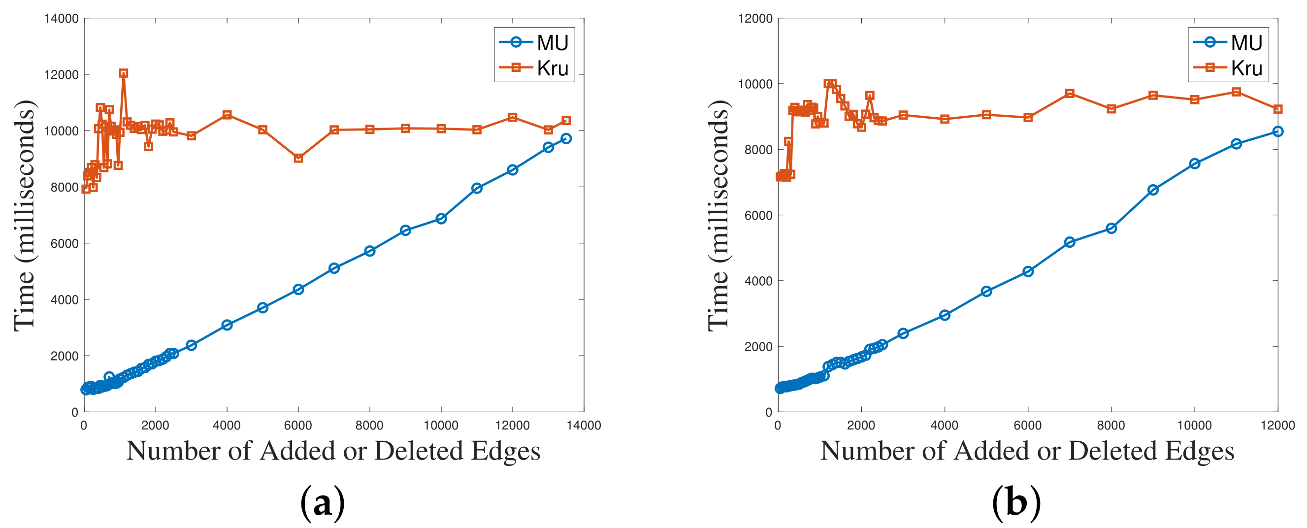
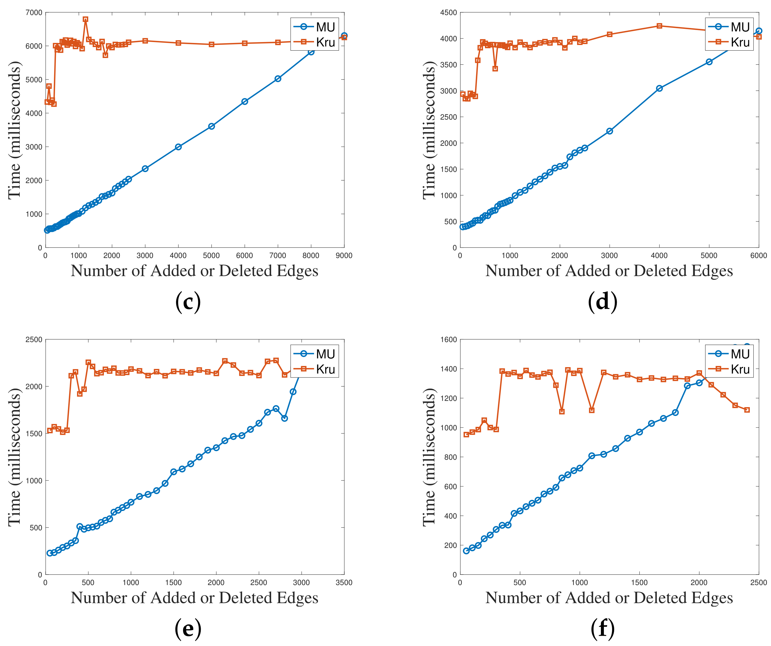
The results are shown in Figure 6. The x-axis in the figures represents the increasing number of added and deleted edges, while the y-axis represents the algorithm’s running time. Through the comparison of the running time results of the six test cases, it was observed that the maintenance algorithm had a significant advantage when the number of modified edges was small. As the number of modified edges increased, the gap between the two algorithms gradually narrowed. When the number of modified edges approached half of the total edges in the test case, the running times of the two algorithms became close. By comparing the figures, we found that with fewer modified edges, an decrease in the graph density led to a greater advantage for the maintenance algorithm.

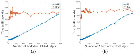
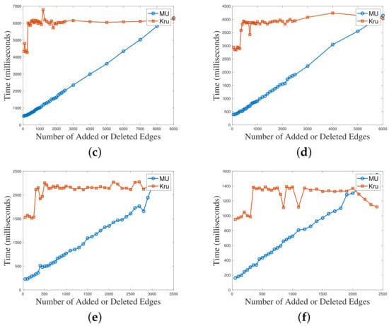
Figure 6. The relationship between algorithm time consumption and graph changes. (a) Range_150_500_1; (b) Range_150_500_3; (c) Range_125_500_3; (d) Range_100_500_3; (e) Range_125_300_1; (f) Range_100_300_1.

6. Conclusions

This paper introduces a dynamic graph minimum spanning tree maintenance algorithm. In the scenario where the original graph and its spanning tree are known, the algorithm quickly solves the minimum spanning tree of a new graph with partial modifications to the original graph. The algorithm also provides an ordered set of the new graph’s edge set to expedite subsequent dynamic minimum spanning tree computations. The paper proves that given the original graph and its spanning tree, the maintenance algorithm yields a correct minimum spanning tree for the new graph. Compared with the traditional Kruskal’s algorithm, the time complexity of the maintenance algorithm is the same as that of Kruskal’s algorithm. This implies that theoretically, the proposed algorithm is on par with the standard Kruskal’s algorithm, which completely recalculates the new graph. In practical execution, the maintenance algorithm efficiently reduces the actual search space, making it more effective for multiple iterations of updates in large-scale graph scenarios. As for future work, we aim to optimize the algorithm’s pruning strategies, for example, maintaining the disjoint-set structure by updating it rather than rebuilding it and using path compression for faster searching. We also hope that the maintenance algorithm proposed in this paper can be extended to more problem domains.

References

- Nesetril, J.; Nesetrilová, H. The origins of minimal spanning tree algorithms—Boruvka and Jarník. Doc. Math. 2012, 17, 127–141. [Google Scholar]
- Lv, X.; Ma, Y.; He, X.; Huang, H.; Yang, J. CciMST: A clustering algorithm based on minimum spanning tree and cluster centers. Math. Probl. Eng. 2018, 2018, 1–14. [Google Scholar] [CrossRef]
- Peter, S.J. Discovering local outliers using dynamic minimum spanning tree with self-detection of best number of clusters. Int. J. Comput. Appl. 2010, 9, 36–42. [Google Scholar] [CrossRef]
- La Grassa, R.; Gallo, I.; Landro, N. OCmst: One-class novelty detection using convolutional neural network and minimum spanning trees. Pattern Recognit. Lett. 2022, 155, 114–120. [Google Scholar] [CrossRef]
- Millington, T.; Niranjan, M. Construction of minimum spanning trees from financial returns using rank correlation. Phys. A Stat. Mech. Its Appl. 2021, 566, 125605. [Google Scholar] [CrossRef]
- Danylchuk, H.; Kibalnyk, L.; Serdiuk, O.; Ivanylova, O.; Kovtun, O.; Melnyk, T.; Zaselskiy, V. Modelling of trade relations between EU countries by the method of minimum spanning trees using different measures of similarity. In Proceedings of the CEUR Workshop Proceedings 2020, Copenhagen, Denmark, 30 March 2020; pp. 167–186. [Google Scholar]
- Xingguo, Y.; Chi, X. The Study of Fund Market Complex Complex Network Based on Cosine Similarity and MST Method. Theory Pract. Financ. Econ. 2020, 41, 55–61. [Google Scholar]
- van Dellen, E.; Sommer, I.E.; Bohlken, M.M.; Tewarie, P.; Draaisma, L.; Zalesky, A.; Di Biase, M.; Brown, J.A.; Douw, L.; Otte, W.M.; et al. Minimum spanning tree analysis of the human connectome. Hum. Brain Mapp. 2018, 39, 2455–2471. [Google Scholar] [CrossRef] [PubMed]
- Chen, J.; Wang, H.; Hua, C.; Wang, Q.; Liu, C. Graph analysis of functional brain network topology using minimum spanning tree in driver drowsiness. Cogn. Neurodyn. 2018, 12, 569–581. [Google Scholar] [CrossRef] [PubMed]
- Jonak, K.; Krukow, P.; Karakuła-Juchnowicz, H.; Rahnama-Hezavah, M.; Jonak, K.E.; Stępniewski, A.; Niedziałek, A.; Toborek, M.; Podkowiński, A.; Symms, M.; et al. Aberrant structural network architecture in Leber’s hereditary optic neuropathy. Minimum spanning tree graph analysis application into diffusion 7T MRI. Neuroscience 2021, 455, 128–140. [Google Scholar] [CrossRef] [PubMed]
- Chreang, S.; Kumhom, P. A Method of Selecting Cable Configuration for Microgrid Using Minimum Spanning Tree. In Proceedings of the 2018 15th International Conference on Electrical Engineering/Electronics, Computer, Telecommunications and Information Technology (ECTI-CON), Chiang Rai, Thailand, 18–21 July 2018; pp. 489–492. [Google Scholar]
- Mosbah, M.; Arif, S.; Mohammedi, R.D.; Hellal, A. Optimum dynamic distribution network reconfiguration using minimum spanning tree algorithm. In Proceedings of the 2017 5th International Conference on Electrical Engineering-Boumerdes (ICEE-B), Boumerdes, Algeria, 29–31 October 2017; pp. 1–6. [Google Scholar]
- Kebir, N.; Ahsan, A.; McCulloch, M.; Rogers, D.J. Modified Minimum Spanning Tree for Optimised DC Microgrid Cabling Design. IEEE Trans. Smart Grid 2022, 13, 2523–2532. [Google Scholar] [CrossRef]
- Ramalingam, G.; Reps, T. On the computational complexity of dynamic graph problems. Theor. Comput. Sci. 1996, 158, 233–277. [Google Scholar] [CrossRef]
- Adasme, P.; de Andrade, R.C. Minimum weight clustered dominating tree problem. Eur. J. Oper. Res. 2023, 306, 535–548. [Google Scholar] [CrossRef]
- Xiong, C.; Liu, H.; Wu, X.; Deng, N. A two-level meta-heuristic approach for the minimum dominating tree problem. Front. Comput. Sci. 2022, 17, 171406. [Google Scholar] [CrossRef]
- Frederickson, G.N. Data structures for on-line updating of minimum spanning trees. In Proceedings of the 15th Annual ACM symposium on Theory of Computing, Boston, MA, USA, 25–27 April 1983; pp. 252–257. [Google Scholar]
- Ribeiro, C.C.; Toso, R.F. Experimental analysis of algorithms for updating minimum spanning trees on graphs subject to changes on edge weights. In Proceedings of the Experimental Algorithms: 6th International Workshop, WEA 2007, Rome, Italy, 6–8 June 2007; Springer: Berlin/Heidelberg, Germany, 2007; pp. 393–405. [Google Scholar]
- Henzinger, M.R.; King, V. Maintaining minimum spanning trees in dynamic graphs. In Proceedings of the Automata, Languages and Programming: 24th International Colloquium, ICALP’97, Bologna, Italy, 7–11 July 1997; Springer: Berlin/Heidelberg, Germany, 1997; pp. 594–604. [Google Scholar]
- Holm, J.; De Lichtenberg, K.; Thorup, M. Poly-logarithmic deterministic fully-dynamic algorithms for connectivity, minimum spanning tree, 2-edge, and biconnectivity. J. ACM (JACM) 2001, 48, 723–760. [Google Scholar] [CrossRef]
- Cattaneo, G.; Faruolo, P.; Petrillo, U.F.; Italiano, G.F. Maintaining dynamic minimum spanning trees: An experimental study. Discret. Appl. Math. 2010, 158, 404–425. [Google Scholar] [CrossRef]
- Eppstein, D.; Galil, Z.; Italiano, G.F.; Nissenzweig, A. Sparsification—a technique for speeding up dynamic graph algorithms. J. ACM (JACM) 1997, 44, 669–696. [Google Scholar] [CrossRef]
- Kopelowitz, T.; Porat, E.; Rosenmutter, Y. Improved worst-case deterministic parallel dynamic minimum spanning forest. In Proceedings of the 30th on Symposium on Parallelism in Algorithms and Architectures, Vienna, Austria, 16–18 July 2018; pp. 333–341. [Google Scholar]
- Tarjan, R.E.; Werneck, R.F. Dynamic trees in practice. J. Exp. Algorithmics (JEA) 2010, 14, 4–5. [Google Scholar]
- Wulff-Nilsen, C. Fully-dynamic minimum spanning forest with improved worst-case update time. In Proceedings of the 49th Annual ACM SIGACT Symposium on Theory of Computing, Montreal, QC, Canada, 19–23 June 2017; pp. 1130–1143. [Google Scholar]
- de Andrade Júnior, J.W.; Duarte Seabra, R. Fully retroactive minimum spanning tree problem. Comput. J. 2022, 65, 973–982. [Google Scholar] [CrossRef]
- Tseng, T.; Dhulipala, L.; Shun, J. Parallel batch-dynamic minimum spanning forest and the efficiency of dynamic agglomerative graph clustering. In Proceedings of the 34th ACM Symposium on Parallelism in Algorithms and Architectures, Philadelphia, PA, USA, 11–14 July 2022; pp. 233–245. [Google Scholar]
- Sundar, S.; Singh, A. New heuristic approaches for the dominating tree problem. Appl. Soft Comput. 2013, 13, 4695–4703. [Google Scholar] [CrossRef]
Disclaimer/Publisher’s Note: The statements, opinions and data contained in all publications are solely those of the individual author(s) and contributor(s) and not of MDPI and/or the editor(s). MDPI and/or the editor(s) disclaim responsibility for any injury to people or property resulting from any ideas, methods, instructions or products referred to in the content. |
© 2024 by the authors. Licensee MDPI, Basel, Switzerland. This article is an open access article distributed under the terms and conditions of the Creative Commons Attribution (CC BY) license (https://creativecommons.org/licenses/by/4.0/).