Abstract
The reconstruction of the spatial complex conductivity from complex valued impedance measurements forms the inverse problem of complex electrical impedance tomography or complex electrical capacitance tomography. Regularized Gauß-Newton schemes have been proposed for their solution. However, the necessary computation of the Jacobian is known to be computationally expensive, as standard techniques such as adjoint field methods require additional simulations. In this work, we show a more efficient way to computationally access the Jacobian matrix. In particular, the presented techniques do not require additional simulations, making the use of the Jacobian, free of additional computational costs.
Keywords:
complex conductivity; quasi-static; FE simulation; Green’s function; Jacobian; tomography; inverse problem MSC:
65M32; 65M80
1. Introduction
In electrical measurements, electrical impedance tomography (EIT) [1], electrical resistance tomography (ERT) [2], and electrical capacitance tomography (ECT) [3,4,5,6,7] form the most established tomographic imaging techniques. The purpose of theses imaging techniques is to visualize the spatial distribution of the conductivity or the relative permittivity within a region of interest (ROI) from electrical measurements. This is done by solving an inverse problem [8,9,10]. The sensor effects are governed by a Laplacian-type partial differential Equation (PDE), i.e., for EIT and ERT and for ECT. V is the electric scalar potential.
Well-known applications of these technique include medical imaging [11] and process tomographic measurements [12], and the application of these sensing techniques to environmental sensing such as monitoring of natural ice accretion [13,14] has also been proposed [15,16,17]. An advantage of electrical imaging systems with respect to other tomographic sensing approaches is the moderate instrumentation effort [18]. A disadvantage is the comparatively low imaging quality, which stems from the soft-field nature of the electric fields within the sensor. Yet, despite the comparatively low imaging quality, electrical tomography systems have seen emerging use as underlying instruments in measurement, e.g., for flow metering of particulate matter in pneumatic conveying [19,20,21,22,23,24,25,26].
The application of EIT, ERT, or ECT requires a dominant conductive or dielectric character of the material distribution within the ROI, i.e., it depends on the ratio , where is the circular frequency and is the absolute permittivity. If , the conductivity is generally imaged. Otherwise, the permittivity is of interest. In applications where holds, it is suitable to solve the inverse problem for both quantities, the conductivity and the relative permittivity . This technique is sometimes referred to as complex electrical impedance tomography (CEIT) [27] or complex electrical capacitance tomography (CECT) [28]. The governing PDE for this problem is given by , which is the quasi-static formulation of the Maxwell equations. The technique must be applied when the complex conductivity () has no dominant dielectric or conductive character, which typically leads to the use of classical ECT [3] or EIT [1] approaches. The joint reconstruction of and is also often considered as an approach for material analysis schemes, making it interesting for different applications.
A common approach for the determination of the material distribution from the measurements is given by [29]
The vectors and are vectors, which hold a discretized representation of the material distributions of the conductivity and the relative permittivity . Throughout this work, an underline notation denotes complex valued variables. denotes an vector of complex impedance measurements. denotes a simulation of the measurement process to compute the M elements of . Hence, the inverse problem consists of determining real-valued parameters from M complex-valued measurements. As the inverse problem formulated by Equation (1) is ill posed [30], a regularization is required [31,32], which we generally denote by , where is a regularization parameter and is a suitable regularization function. Often Equation (1) is augmented by constraints particular to the measurement application.
In this work, we use a finite element (FE) approach for the computation of . Here, it is common to use the FE discretization of the sensing region to create the vectors and . Solving Equation (1) can be efficiently done using first- or second-order optimization methods [33,34], which require the Jacobian . The elements of are the derivatives of the outputs of with respect to the optimization variables. Because of the complex valued measurements the Jacobian is given by [29]
where and denote the Jacobian of the model outputs with respect to the elements of and , respectively. In addition to a numerical computation of the Jacobian by means of a difference scheme, there exist several techniques such as sensitivity methods [35], or adjoint field methods [36] to compute . From the computational point of view, these methods require an additional simulation with the effort equivalent to the evaluation of , i.e., another FE equation system has to be solved [37]. This makes the evaluation of the Jacobian computationally costly, which is a crucial factor for the fast solution of inverse problems.
In a previous study [38], our research group showed a set of fast numerical techniques for the solution of the inverse problem of ECT. This includes a fast technique for the assembly of the FE stiffness matrix and, in particular, a set of techniques to evaluate matrix vector products with the Jacobian or its transpose without an explicit evaluation of . No additional computations are required. These so-called Jacobian operations are enabled by a simulation approach using Green’s functions [39], which is possible due to the symmetry of the real-valued FE stiffness matrix. However, for the complex-valued FE stiffness matrix of the computation , a Green’s function approach is not directly applicable, as the matrix would be required to be Hermitian [39].
In this work, an extension of the fast numerical techniques for inverse problems with an underlying quasi-static electrical field problem is presented. The novelty and contributions of the work are given by the following:
- Derivation of a solution approach with Green’s functions for the quasi-static field problem;
- A technique to compute the full Jacobian in one step. Unlike existing methods, the new approach requires no additional simulations;
- The formulation of the inverse problem Equation (1) to efficiently use the derived techniques.
A strength of the work lies in the consistent use of linear algebra techniques throughout all derivations, as well as for the representation of the final computations. This allows researchers to utilize a direct implementation within their individual code. In addition, a MATLAB-based implementation of the methods is provided via a GitHub repository.
The rest of this paper is structured as follows. Section 2 presents a recap of the methods presented in [38], including an introduction to the considered sensor setup. In Section 3, the application of the Green’s function approach to inverse problems with an underlying quasi-static electrical field problem is shown. Here, the required computations with respect to the real-valued counterpart presented in [38] are derived. Afterward, the computational steps to solve inverse problems with the new methods are discussed. Section 4 presents an example and computational speed comparisons of the methods with respect to a reference solution.
2. Fast Numerical Techniques for Symmetric Real-Valued Problems
This section contains a summary of the fast numerical techniques presented in [38]. While the techniques were developed for the inverse problem of ECT, most aspects can be related to the complex-valued problems treated in this work.
Figure 1 depicts the scheme of an ECT sensor as it is used in industrial process tomography. The sensor is assembled around a non-conductive pipe. The sensing electrodes are mounted on the outside of the pipe and the whole assembly is shielded by a screen. The domain inside the shield is denoted as . The shield forms the boundary . The measurements are given by the capacitances between the electrodes, which depend on the material distribution inside the pipe. This domain is denoted as of the sensor.
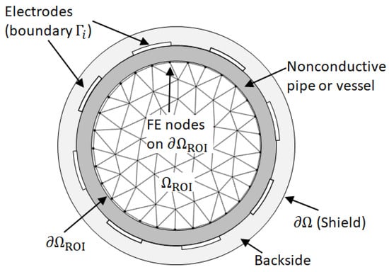
Figure 1.
Scheme of a tomographic sensor for process tomography.
The simulation model for ECT is denoted by . It comprises the solution of the PDE . The boundary conditions on the electrodes and on the screen are of the Dirichlet type. The potential of one electrode is set to , while the potentials for all other electrodes and the screen are set to . Hence, the PDE has to be solved times. Using the FE method, this results in the FE equation system
Here, is the sparse symmetric and real-valued FE stiffness matrix. is the number of nodes of the FE mesh. The hat symbol indicates the incorporation of the boundary conditions. In this work, the technique of keeping the essential nodes is used [40]. is an vector holding the permittivity values for the finite elements in the ROI as depicted in Figure 1. The matrix is of the dimension and holds the boundary conditions for the electrode excitation patterns of the measurements. is the corresponding solution vector holding the nodal potentials. Hence, is of the same dimension as .
After solving Equation (3) for , the coupling capacitances between the electrodes are computed by the integration of the displacement flux for each electrode. The fluxes are then normalized by , leading to the capacitances. Following [38], the normalization by is skipped, which means that the charges on the electrodes are computed. Using the FE discretization, these computations can be performed by
where is a matrix of dimension and is an matrix. For each excitation, the charges for each electrode are held in the columns of the matrix , i.e., , where j denotes the electrode where the excitation is applied and i is the electrode where the flux is integrated. The M measurements are taken from the elements of .
In the following, the main computational results of [38] are summarized.
2.1. Fast Assembly of the Stiffness Matrix and Modified Charge Computation
The assembly of is a well-known bottleneck within FE simulations. To overcome this, the assembly is carried out by
Here, holds the constant part of the matrix , including the incorporation of the boundary conditions. p is the order of the finite elements. The columns of the matrices are formed from the eigenvectors of the FE element matrices and their eigenvalues. As the FE element matrices are rank deficient, only matrices are required. The entries within the columns of are arranged by means of the global node number. Hence, the matrices are sparse matrices.
For the computation of , Equation (4) is split into
Here, is evaluated from the potential on , which is the potential on the boundary of the ROI. represents the charges for the domain .
The initial setup costs for the proposed technique require an eigenvector decomposition of the FE element matrices for the assembly of the matrices and the computation of and . Yet, as discussed in [38], the benefit of the stiffness matrix assembly technique following Equation (5) is given by the superior speedup with respect to other techniques.
2.2. Solution with Green’s Functions
Instead of solving Equation (3) for , the equation system
is solved for , which are referred to as Green’s functions for . The matrix holds the identity vectors for the nodes on . By multiplication with , Equation (7) has the same dimensions as the original FE equation system given by Equation (3). Given , Equation (6) can be replaced by
to compute the charges.
2.3. Jacobian Operations
The solution by Green’s functions is possible due to the symmetry of the FE stiffness matrix . Yet, Green’s functions can be used to replace the inverse of [38,39]. For the presented inverse problem with the simulation model , this allows the derivation of the Jacobian operation as
and the transpose of the Jacobian operation as
Equation (9) allows the computation of the matrix vector product without an explicit evaluation of the Jacobian . The evaluation of provides a local linear approximation model for . An application for the Jacobian operation are Markov Chain Monte Carlo (MCMC) techniques [41,42,43].
In the transpose of the Jacobian operation provided by Equation (10), ⊙ denotes a row- and column-wise multiplication, and the matrix is assembled from the residual vector . The transpose of the Jacobian operation provides the local gradient for the objective function . Hence, it is essential for the solution of inverse problems as formulated by Equation (1).
3. Green’s Function Approach for Quasi-Static Problems
In this section, the extension of the techniques presented in Section 2.1 for quasi-static problems is shown. The governing PDE in the sensor is given by . The inverse problem aims for the combined reconstruction of the conductivity and the relative permittivity .
With the FE method, the computations in are given by
Here, the underline notation expresses the complex-valued nature of the terms. In the following, we skip the input arguments for the FE stiffness matrix for better readability. For complex-valued and Hermitian matrices a Green’s function approach for the rows of the matrix can be applied by
Here, is the matrix holding the identity vectors for the elements held in , and denotes the Hermitian of . However, the FE modeling approach generally leads to non-Hermitian matrices, i.e., holds. Thus, the Green’s function approach can formally not be applied [39].
3.1. Green’s Functions for the Quasi-static Formulation
To apply a Green’s function approach, we left-multiply Equation (11) by . This gives
As the matrix is real-valued and symmetric, a Green’s function approach can be applied as
to compute by .
This gives
From Equation (13), it can be seen that corresponds to the Green’s functions , as holds. Thus, a Green’s function approach can be applied for non-Hermitian matrices by
Given this result, all of the presented techniques addressed in Section 2.1 can be used, by applying the transpose for the Green’s functions. The computations for are, therefore, given by
and
to compute the measurements.
3.2. Jacobian Operations for the Quasi-Static Field Problem
In the previous section, the applicability of a Green’s function approach for quasi-static field problems was derived. This enables the use of Jacobian operations to speed up the solution of Equation (1). However, this still requires some modifications in the formulation of the problem. Throughout the remaining part of this work, the following notation is used. Vectors marked with an underline are complex-valued vectors, e.g., . Their real-valued counterparts are denoted without the underline and formed by .
While the inverse problem formulated by Equation (1) maintains the vectors and as optimization variables, in this work the complex-valued vector is used.
Hence, the real part of represents the distribution of and the imaginary part represents the distribution of .
Hence, the inverse problem can be formulated as
where a single Tikhonov-type [44] regularization is used. As the real and the imaginary part of are of the same magnitude, a joint regularization with a single regularization parameter can be applied. Furthermore, the inverse problem is augmented by boxed constraints.
For a first-order optimization scheme, the gradient of the objective function in Equation (26) is required, which is given by
The product of can now be evaluated using the transpose of the Jacobian operation
where is the complex-valued representation of . The matrix is formed from the complex-valued vector . Thus, the gradient in Equation (27) can be directly evaluated from the solution of , which gives the Green’s functions .
For a second-order optimization scheme, the Hessian matrix
has to be computed, which requires an explicit evaluation of the Jacobian . Using Equation (28), the complex-valued Jacobian can be assembled in a sequential way by setting the elements in to 1. The real-valued Jacobian is then given by
This procedure requires M evaluations of Equation (28). However, by using MATLAB’s vector indexing scheme, the matrix can be constructed in one step using Equation (28). To access this, the matrix
is used, which shows the numbering scheme of the elements held in the matrix , or , respectively. The column vector now holds the column-wise sequence of the indices held in the matrix for the M measurements. The vector is of the same dimension and holds the corresponding column numbers for each element of . By defining the matrix , the Jacobian can be evaluated by
where and express MATLAB’s matrix indexing scheme. We refer to this technique as fast Jacobian. Note that the matrix is stored as a sparse matrix. For the evaluation of Equation (30), it is suitable to create full matrices, since the evaluation of Equation (29) is faster.
Jacobian Operation
While it is not used for the solution of the inverse problem stated by Equation (26), the Jacobian operation can also be applied to the quasi-static problem. It is given by
presents the variation for the vector , for which the Green’s functions have been computed. holds the variation due to in matrix form.
4. Reconstruction Example and Computational Speed Comparison
In this section, a numerical study of the proposed methods is presented. The focus of the analysis lies on the comparison of the computational speed improvement. Therefore, a first-order method based on BFGS and a second-order Gauss Newton (GN) method are used to solve the inverse problem formulated by Equation (26). As a reference technique for the computation of the Jacobian, the technique presented in [36] is used, which is referred to as the adjoint variable method (AVM).
The following computations are implemented:
- GN-based optimization with Jacobian computation based on AVM;
- GN-based optimization with fast Jacobian computation;
- BFGS-based optimization with fast Jacobian computation;
- BFGS-based optimization with transpose of Jacobian operation.
For the GN-based techniques, MATLAB’s fmincon is used. In combination with the Jacobian computation using the AVM method, this technique provides the established reference technique. For the BFGS-based techniques, we used a MATLAB implementation provided by [45]. The simulation study is carried out for a sensor as depicted in Figure 1 with electrodes. The ROI for this example contains finite elements. Since the study focuses on the computational speed, the same simulation model is used for both the data generation and the image reconstruction. For the regularization, a second-order smoothness matrix is used for the real part and the imaginary part of . The measurement frequency is set to . Box constraints with and are applied to all of the four implementations. The MATLAB code is provided under the link given at the end of the paper.
Figure 2 and Figure 3 show two exemplary image reconstruction results using GN-based techniques, which illustrate the functionality of the proposed approach. The figures show the true material distribution as well as the corresponding reconstruction results. In the first reconstruction experiment, a layer of higher conductivity and higher relative permittivity is placed at the lower half of the pipe. The true material distributions also show the FE discretization. In the reconstruction results, the effect of the prior smoothing is visible. Yet, both reconstruction results provide a meaningful representation of the true distribution. Similar results are obtained for the second reconstruction experiment depicted in Figure 3, where a circular inclusion in the center of the pipe is studied. The regularization parameter was determined based on an L-curve evaluation as depicted in Figure 4.
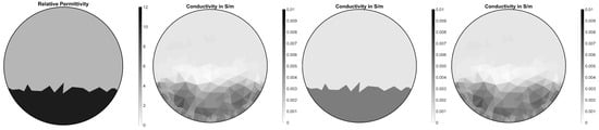
Figure 2.
Reconstruction example 1.
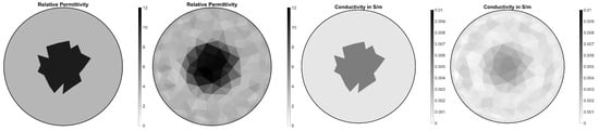
Figure 3.
Reconstruction example 2.
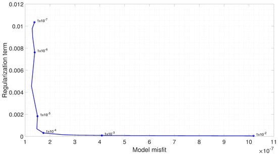
Figure 4.
L-curve for the determination of the regularization parameter .
Figure 5 shows the convergence behavior of the different GN- and BFGS-based techniques. The results have been computed for the material distribution presented in Figure 2. The two GN approaches and the two BFGS approaches show identical convergence behavior. The four methods lead to numerically equivalent reconstruction results, i.e., the differences are in the order of magnitude of numerical rounding errors. For the GN-based techniques, a faster convergence is achieved, which is due to the incorporation of the Hessian matrix. The BFGS algorithm iteratively approximates the inverse Hessian [33], which leads to a slightly slower convergence.
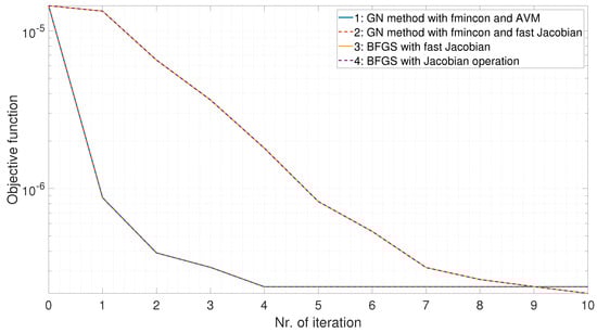
Figure 5.
Convergence behavior of the different GN and BFGS implementations.
While the different implementations lead to the same numerical values, the different computational methods for the Jacobian lead to significant differences in the computation times. Figure 6 shows a timing comparison for the four different methods. For the first three methods, where the Jacobian is explicitly formed, the first iteration lasts longer due to the initial storage acquisition. The benefit of the fast Jacobian technique with respect to the reference AVM method is evident, as can be seen by the comparison between the first and the second method.
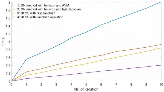
Figure 6.
Timing comparison between different optimization schemes and different techniques for the evaluation of the Jacobian. The first technique (GN method with fmincon and AVM) uses the established AVM technique for the computation of the Jacobian. The other techniques use the proposed techniques for fast computations with the Jacobian.
The third method using the BFGS approach is slightly faster than the second, GN-based, method. From profiling, we found the time difference between the second and the third method to be caused by the evaluation of in Equation (29). The fourth method does not require an explicit evaluation of the Jacobian, as the gradient stated by Equation (27) is computed by the transpose of Jacobian operation. The benefit of the method is obvious with respect to the computation time. Another positive aspect is given by the reduced storage requirements, as the fourth algorithm does not require the storage of . The results presented in this section highlight the benefit of the proposed numerical methods. The presented study was conducted for . Tests with different values of N did not show any limitations to the approach.
5. Conclusions
In this work, the application of a Green’s function approach for FE simulations in quasi-static field problems has been presented. The modification with respect to real-valued problems was derived. Based on the analysis, the application to other problems should also be possible. Using the Green’s functions, efficient methods for computations using the Jacobian are derived. This includes Jacobian and transpose of Jacobian operations, as well as a technique to assemble the whole Jacobian in one step. A benefit of all the derived methods is the use of linear algebra expressions, which allow a convenient re-implementation by researchers and engineers in the field.
Author Contributions
Conceptualization, M.N. and T.S.; methodology, M.N.; software, M.N.; validation, M.N., T.S. and C.F.; formal analysis, M.N., T.S. and C.F.; investigation, M.N.; writing—original draft preparation, M.N.; writing—review and editing, M.N. and T.B. and H.W.; visualization, M.N.; project administration, M.N. and H.W.; funding acquisition, H.W. All authors have read and agreed to the published version of the manuscript.
Funding
The financial support by the Austrian Federal Ministry for Digital and Economic Affairs, the National Foundation for Research, Technology and Development, and the Christian Doppler Research Association is gratefully acknowledged. Supported by TU Graz Open Access Publishing Fund.
Data Availability Statement
An exemplary MATLAB implementation of the presented methods is provided under the GitHub account /neumayerm/OIPE_2023.
Conflicts of Interest
The authors declare no conflicts of interest.
Abbreviations
The following abbreviations are used in this manuscript:
| AVM | Adjoint Variable Method |
| BFGS | Broyden–Fletcher–Goldfarb–Shanno |
| EIT | Electrical impedance tomography |
| ERT | Electrical resistance tomography |
| ECT | Electrical capacitance tomography |
| FE | Finite Element |
| GN | Gauss Newton |
| PDE | Partial Differential Equation |
References
- Holder, D.S. Electrical Impedance Tomography: Methods, History and Applications; Institute of Physics Publishing: Philadelphia, PA, USA, 2005. [Google Scholar]
- Scott, D.M.; McCann, H. Process Imaging For Automatic Control (Electrical and Computer Enginee); CRC Press, Inc.: Boca Raton, FL, USA, 2005. [Google Scholar]
- Neumayer, M.; Steiner, G.; Watzenig, D. Electrical Capacitance Tomography: Current sensors/algorithms and future advances. In Proceedings of the 2012 IEEE International Instrumentation and Measurement Technology, Graz, Austria, 13–16 May 2012; pp. 929–934. [Google Scholar] [CrossRef]
- Jaworski, A.J.; Dyakowski, T. Application of electrical capacitance tomography for measurement of gas-solids flow characteristics in a pneumatic conveying system. Meas. Sci. Technol. 2001, 12, 1109–1119. [Google Scholar] [CrossRef]
- Cui, Z.; Wang, Q.; Xue, Q.; Fan, W.; Zhang, L.; Cao, Z.; Sun, B.; Wang, H.; Yang, W. A review on image reconstruction algorithms for electrical capacitance/resistance tomography. Sens. Rev. 2016, 36, 429–445. [Google Scholar] [CrossRef]
- Wang, H.; Yang, W. Application of electrical capacitance tomography in circulating fluidised beds—A review. Appl. Therm. Eng. 2020, 176, 115311. [Google Scholar] [CrossRef]
- Wang, H.; Yang, W. Scale-up of an electrical capacitance tomography sensor for imaging pharmaceutical fluidized beds and validation by computational fluid dynamics. Meas. Sci. Technol. 2011, 22, 104015. [Google Scholar] [CrossRef]
- Tarantola, A. Inverse Problem Theory and Methods for Model Parameter Estimation; Society for Industrial and Applied Mathematics: Philadelphia, PA, USA, 2004. [Google Scholar]
- Kaipio, J.; Somersalo, E. Statistical and Computational Inverse Problems; Springer Applied Mathematical Sciences: Philadelphia, PA, USA, 2005. [Google Scholar]
- Neumayer, M.; Bretterklieber, T.; Flatscher, M.; Puttinger, S. PCA based state reduction for inverse problems using prior information. COMPEL Int. J. Comput. Math. Electr. Electron. Eng. 2017, 36, 1430–1441. [Google Scholar] [CrossRef]
- Adler, A. Electrical Impedance Tomography: Methods, History and Applications, 2nd ed.; CRC Press: Boca Raton, FL, USA, 2021. [Google Scholar]
- Wang, M. Industrial Tomography: Systems and Applications, 2nd ed.; Woodhead Publishing Series in Electronic and Optical Materials; Woodhead Publishing: Sawston, UK, 2022. [Google Scholar]
- Kang, G.; Hongfei, B.; Ziyu, L.; Junfeng, G.; Lin, Y. Impedance Ice Sensor Capable of Self-Componsating Temperature Drift. In Proceedings of the 2023 IEEE 16th International Conference on Electronic Measurement and Instruments (ICEMI), Harbin, China, 9–11 August 2023; pp. 118–122. [Google Scholar] [CrossRef]
- Dean, R.N. A PCB Sensor for Detecting Icing Events. IEEE Sens. Lett. 2021, 5, 1–4. [Google Scholar] [CrossRef]
- Zheng, D.; Li, Z.; Du, Z.; Ma, Y.; Zhang, L.; Du, C.; Li, Z.; Cui, L.; Zhang, L.; Xuan, X.; et al. Design of Capacitance and Impedance Dual-Parameters Planar Electrode Sensor for Thin Ice Detection of Aircraft Wings. IEEE Sens. J. 2022, 22, 11006–11015. [Google Scholar] [CrossRef]
- Gui, K.; Liu, J.; Ge, J.; Li, H.; Ye, L. Atmospheric icing process measurement utilizing impedance spectroscopy and thin film structure. Measurement 2022, 202, 111851. [Google Scholar] [CrossRef]
- Flatscher, M.; Neumayer, M.; Bretterklieber, T.; Moser, M.J.; Zangl, H. De-icing system with integrated ice detection and temperature sensing for meteorological devices. In Proceedings of the 2015 IEEE Sensors Applications Symposium (SAS), Zadar, Croatia, 13–15 April 2015; pp. 1–6. [Google Scholar] [CrossRef]
- Wang, B.; Huang, Z.; Li, H. Design of high-speed ECT and ERT system. J. Phys. Conf. Ser. 2009, 147, 012035. [Google Scholar] [CrossRef]
- Maung, C.O.; Kawashima, D.; Oshima, H.; Tanaka, Y.; Yamane, Y.; Takei, M. Particle volume flow rate measurement by combination of dual electrical capacitance tomography sensor and plug flow shape model. Powder Technol. 2020, 364, 310–320. [Google Scholar] [CrossRef]
- Datta, U.; Dyakowski, T.; Mylvaganam, S. Estimation of particulate velocity components in pneumatic transport using pixel based correlation with dual plane ECT. Chem. Eng. J. 2007, 130, 87–99. [Google Scholar] [CrossRef]
- Neumayer, M.; Flatscher, M.; Bretterklieber, T. Coaxial Probe for Dielectric Measurements of Aerated Pulverized Materials. IEEE Trans. Instrum. Meas. 2019, 68, 1402–1411. [Google Scholar] [CrossRef]
- Wang, D.; Xu, M.; Marashdeh, Q.; Straiton, B.; Tong, A.; Fan, L.S. Electrical capacitance volume tomography for characterization of gas–solid slugging fluidization with Geldart group D particles under high temperatures. Ind. Eng. Chem. Res. 2018, 57, 2687–2697. [Google Scholar] [CrossRef]
- Rasel, R.K.; Chowdhury, S.M.; Marashdeh, Q.M.; Teixeira, F.L. Review of selected advances in electrical capacitance volume tomography for multiphase flow monitoring. Energies 2022, 15, 5285. [Google Scholar] [CrossRef]
- Zhang, W.; Wang, C.; Yang, W.; Wang, C.H. Application of electrical capacitance tomography in particulate process measurement—A review. Adv. Powder Technol. 2014, 25, 174–188. [Google Scholar] [CrossRef]
- Huang, K.; Meng, S.; Guo, Q.; Ye, M.; Shen, J.; Zhang, T.; Yang, W.; Liu, Z. High-temperature electrical capacitance tomography for gas–solid fluidised beds. Meas. Sci. Technol. 2018, 29, 104002. [Google Scholar] [CrossRef]
- Yang, W.; Wang, H. Application of electrical capacitance tomography in pharmaceutical manufacturing processes. In Proceedings of the 2019 IEEE International Instrumentation and Measurement Technology Conference (I2MTC), Auckland, New Zealand, 20–23 May 2019; pp. 1–6. [Google Scholar]
- Jiang, Y.; Soleimani, M. Capacitively Coupled Phase-based Dielectric Spectroscopy Tomography. Sci. Rep. 2018, 8, 17526. [Google Scholar] [CrossRef] [PubMed]
- Jossinet, J.; Trillaud, C. Imaging the complex impedance in electrical impedance tomography. Clin. Phys. Physiol. Meas. 1992, 13, 47. [Google Scholar] [CrossRef] [PubMed]
- Hollaus, K.; Gerstenberger, C.; Magele, C.; Hutten, H. Accurate reconstruction algorithm of the complex conductivity distribution in three dimensions. IEEE Trans. Magn. 2004, 40, 1144–1147. [Google Scholar] [CrossRef]
- Hansen, P.C. Rank-Deficient and Discrete Ill-Posed Problems: Numerical Aspects of Linear Inversion; Society for Industrial and Applied Mathematics (SIAM): Philadelphia, PA, USA, 1998. [Google Scholar]
- Engl, H.W.; Hanke, M.; Neubauer, A. Regularization of Inverse Problems; Kluwer Verlag: Philadelphia, PA, USA, 2002. [Google Scholar]
- Kaipio, J.; Somersalo, E. Statistical and Computational Inverse Problems, 1st ed.; Springer: Berlin/Heidelberg, Germany, 2004. [Google Scholar]
- Fletcher, R. Practical Methods of Optimization, 2nd ed.; Wiley-Interscience: New York, NY, USA, 1987. [Google Scholar]
- Nocedal, J.; Wright, S.J. Numerical Optimization, 2nd ed.; Springer: New York, NY, USA, 2006. [Google Scholar]
- Geselowitz, D.B. An Application of Electrocardiographic Lead Theory to Impedance Plethysmography. IEEE Trans. Biomed. Eng. 1971, BME-18, 38–41. [Google Scholar] [CrossRef]
- Brandstätter, B. Jacobian calculation for electrical impedance tomography based on the reciprocity principle. IEEE Trans. Magn. 2003, 39, 1309–1312. [Google Scholar] [CrossRef]
- Brančík, L. Comparative Study of Jacobian Calculation Techniques in Electrical Impedance Tomography. In Proceedings of the VI. International Workshop “Computational Problems of Electrical Engineering”, Kynżvart, Czech Republic, 13–16 September 2004; p. 101. [Google Scholar]
- Neumayer, M.; Suppan, T.; Bretterklieber, T.; Wegleiter, H.; Fox, C. Fast Numerical Techniques for FE Simulations in Electrical Capacitance Tomography. In Proceedings of the 20th International IGTE Symposium on Computational Methods in Electromagnetics and Multiphysics, Graz, Austria, 18–21 September 2022. [Google Scholar] [CrossRef]
- Young, N. An Introduction to Hilbert Space; Cambridge University Press: New York, NY, USA, 1988. [Google Scholar]
- Ern, A.; Guermond, J. Theory and Practice of Finite Elements; Applied Mathematical Sciences; Springer: New York, NY, USA, 2004. [Google Scholar]
- Gilks, W. and Richardson, S. and Spiegelhalter, D. Markov Chain Monte Carlo in Practice: Interdisciplinary Statistics; Chapman and Hall/CRC: Boca Raton, FL, USA, 1995. [Google Scholar]
- Watzenig, D.; Neumayer, M.; Fox, C. Accelerated Markov chain Monte Carlo sampling in electrical capacitance tomography. Int. J. Comput. Math. Electr. Electron. Eng. 2011, 30, 1842–1854. [Google Scholar] [CrossRef][Green Version]
- Christen, J.A.; Fox, C. Markov chain Monte Carlo Using an Approximation. J. Comput. Graph. Stat. 2005, 14, 795–810. [Google Scholar] [CrossRef]
- Vogel, C.R. Computational Methods for Inverse Problemss; Society for Industrial and Applied Mathematics (SIAM): Philadelphia, PA, USA, 2002. [Google Scholar]
- Granzow, B. A Matlab Implementation of L-BFGS-B. 2017. Available online: https://github.com/bgranzow/L-BFGS-B (accessed on 23 January 2024).


Disclaimer/Publisher’s Note: The statements, opinions and data contained in all publications are solely those of the individual author(s) and contributor(s) and not of MDPI and/or the editor(s). MDPI and/or the editor(s) disclaim responsibility for any injury to people or property resulting from any ideas, methods, instructions or products referred to in the content. |
© 2024 by the authors. Licensee MDPI, Basel, Switzerland. This article is an open access article distributed under the terms and conditions of the Creative Commons Attribution (CC BY) license (https://creativecommons.org/licenses/by/4.0/).