A Source Identification Problem in Magnetics Solved by Means of Deep Learning Methods

Abstract

In this study, a deep learning-based approach is used to address inverse problems involving the inversion of a magnetic field and the identification of the relevant source, given the field data within a specific subdomain. Three different techniques are proposed: the first one is characterized by the use of a conditional variational autoencoder (CVAE) and a convolutional neural network (CNN); the second one employs the CVAE (its decoder, more specifically) and a fully connected deep artificial neural network; while the third one (mainly used as a comparison) uses a CNN directly operating on the available data without the use of the CVAE. These methods are applied to the magnetostatic problem outlined in the TEAM 35 benchmark problem, and a comparative analysis between them is conducted.

1. Introduction

1.1. Overview

In recent years, extensive research efforts have focused on employing neural network (NN)-based methods to deal with electromagnetic (EM) field problems. This paper proposes and compares various deep learning (DL)-based approaches for solving an inverse problem in magnetostatics. In particular, this work is the continuation of the research activity carried out by the authors, with the main goals of highlighting the difference between different NN/DL-based approaches; the comparison is made both in terms of computational resources and in the accuracy of the obtained results. Such comparisons on a specific test case have been rarely presented in the literature.

Source identification and field reconstruction are fundamental aspects in EM field research; besides being theoretically sound, such kinds of inverse problems also find applications in many different high-technology environments [1,2,3].

1.2. Literature Review

In introducing NNs in EM solvers, frequently taking the form of DL models, NNs have found applications mainly in addressing direct EM problems. This is especially valuable when optimization processes necessitate numerous field computations [4,5]: their primary advantage lies in their capability to accurately assess desired parameters in reduced computational time. This can be accomplished by effectively training the NN with an appropriate dataset. Nevertheless, it is crucial to know that the effort associated with the generation of the training dataset (including the time required for constructing the dataset and model) is a non-negligible factor that needs to be considered in the overall assessment of DL’s effectiveness in solving EM problems.

A newer application of DL arises from the ability to train NNs to address inverse EM problems. This involves identifying the magnitude and/or the geometric characteristics of the source when the field distribution is known at specific locations [6]. It must be highlighted that EM forward problems are commonly well posed and associated with unicity of the solution, achievable with a certain level of approximation determined by the numerical method used for the solution, if the sources and boundaries are well defined. In contrast, inverse problems are typically addressed by minimizing a field reconstruction error, and regularization techniques are frequently needed in this context due to the inherent non-uniqueness and ill-conditioned nature of raw observed data.

In this context, the employment of DL for EM problem inversion basically corresponds to the application of a regularization technique. Several authors have explored similar concepts in areas such as image processing [7,8,9,10,11,12,13]; however, the specific application of DL for solving inverse problems in electromagnetic fields remains a relatively unexplored area, with several aspects still to be investigated [4,5,6].

Both in forward and inverse solutions, DL offers an interesting advantage: the ability to work directly with images. This means that various elements such as geometry (including boundaries and material interfaces), sources, and outcomes (such as field distributions represented as color maps) can be efficiently and directly represented using images.

In a previous work [13], the authors proposed a DL approach for 2D field reconstruction and source identification, where the available data were the magnetic field in a specific sub-region of space Ω₀. The main goal was to find either the field distribution in the whole domain Ω or the geometry of the sources (or to solve both problems at the same time). The model proposed in [13] is composed of a cascade of a conditional variational autoencoder (CVAE) [14,15] and a convolutional neural network (CNN) [11], where the CVAE reconstructs the field distribution in the whole domain Ω given the field in a subdomain Ω₀, and the CNN predicts the device geometry given the output reconstructed field of the CVAE. The approach proposed in [13] was applied to the EM problem as presented in TEAM 35 [16,17].

1.3. Motivation

In this work, the authors were interested in presenting, analyzing, and comparing other approaches with respect to those in [13]. The use of ML-based approaches is a “trending topic” in many research areas, and in the authors’ opinion, there are several good contributions like the ones cited above; however, the wide variety of approaches and test cases results in an objective difficulty in comparing their performances and their positive and negative aspects. In the present contribution, the authors propose a clear comparison between different methods, starting with using the same physical EM problem and the same database.

To this extent, three different approaches are compared. The first approach is the one proposed in [13], for which updated results are reported in this work, resulting from a more efficient training. The motivation for the choice of the methodology lies in the fact that the CVAE is a powerful generative DL method, which is effective in reconstructing the field image distribution in the full domain knowing the field distribution in a subdomain. Additionally, a CNN can be used as a regressor to obtain the sources from a reconstructed field image. The second approach consists of substituting both the decoder part of the CVAE and the subsequent CNN with a fully connected artificial neural network, denoted as ANN, to identify the sources. In this approach, the authors still employed the low dimensional data lying in the latent space defined by the CVAE encoder as an input of the ANN, taking fully advantage of the CVAE’s capability of representing high-dimensional images in a low-dimensional space. As a third approach, an evaluation of the sources was performed directly from the field data in the sub-region Ω₀ through the use of a CNN. Approaches 2 and 3 aimed to only identify the source, while Approach 1 is the only one that also solves the problem of field reconstruction.

The remaining parts of this paper are organized as follows. In Section 2, the use of the CVAE for field reconstruction is presented and motivated, along with a description of the latent space solution that was optimized using automatic differentiation. Also in Section 2, the three DL approaches for source identification are further presented. In Section 3, the TEAM 35 case study is described, while Section 4 is dedicated to the results. Finally, in Section 5, a discussion and conclusion are reported.

2. Deep Learning Models for Field Reconstruction and Source Identification

It is assumed that the field source is an arbitrary distribution of current-carrying conductors in air. Three possible approaches to field inversion are proposed here.

2.1. Conditional Variational Autoencoder

An autoencoder (AE) is an unsupervised learning technique [11], and its primary function is to compress images and reconstruct them from the reduced representation, usually called the latent space. An AE is composed of two neural networks: an encoder and a decoder. The encoder transforms the input image $X$ (usually a two-dimensional matrix) into a vector $Z$ of reduced dimensions (with respect to the original image). Subsequently, the decoder utilizes this condensed representation to reconstruct the original image as X_rec, aiming to minimize the reconstruction error. Due to this error in the reconstruction, the encoder performs what is known as lossy compression—essentially removing certain information during the compression process.

In a variational autoencoder (VAE) [12], the encoder produces two output vectors of dimension $n_L$, i.e., the mean value ${\mu }_z$ and the standard deviation ${\sigma }_z$, that describe the probability distribution associated with $Z$, rather than produce a single $Z$ point as in the case of the standard autoencoder. The values ${\mu }_z$ and ${\sigma }_z$ represent the probability distribution of the latent representation of X, essentially reflecting how the encoder discerns the posterior distribution $p\left(Z|X\right)$.

The probability distribution, crucial in the operation of the decoder, makes it possible to extract a point $Z$ within the latent space as follows:

$$Z~q\left(Z|X\right)={\mu }_z+ϵ{\sigma }_z$$

(1)

with $ϵ~\mathcal{N}\left(\mathrm{0,1}\right)$ and $q\left(Z|X\right)$ being the approximate posterior distribution. The sampled $Z$ point is given to the decoder, which operates as in the case of the standard autoencoder, i.e., generating the reconstructed image X_rec. The VAE loss involves two parts: the reconstruction loss, measuring the difference between original image X and decoded image X_rec, and the Kullback–Leibler loss [14], which aligns learned means and variances with a normal distribution. Balancing these errors creates a smoother, more organized latent space compared to standard autoencoders, which minimize only reconstruction errors. This is crucial for generative models, which aim to generate new data.

In a CVAE [15], a special “label” variable, denoted as Y, is used. It is an extra input that acts as a guide to how X is encoded and reconstructed in the CVAE. In this specific study, X represents the magnetic field map over the entire domain Ω, while Y depicts the map in a smaller region Ω₀ within X. The goal is to reconstruct X using only Y. From a mathematical viewpoint, the problem is ill posed due to a lack of knowledge on the boundary conditions in Ω₀; nevertheless, utilizing a CVAE is a way of regularizing the problem in the search for a solution [13]. During the training, both image X and label Y are inputs of the CVAE, while during the test, only the label Y is given to the decoder.

When reconstructing a field map without direct encoder input X during the test Dphase and prediction phase, the decoder still needs an estimate of the latent space mapping $Z$ corresponding to unknown image X. For this purpose, a rough estimate, denoted as X₀, can be randomly guessed, or selected by picking the most similar example belonging to the training set, leveraging the conditioning with Y. Once X₀ is selected, the corresponding $Z_0$ is consequently estimated using the encoder. The authors verified that further refining the $Z_0$ latent space solution improves the reconstruction; for this reason, an optimization process is performed for the definition of the best $Z$ solution, using automatic differentiation and the gradient descent algorithm [13]. The objective function used here is the mean of squared errors:

$${mse}_Y\left(Z_k\right)=\frac{{‖Y-Y_k\left(Z_k\right)‖}_F^2}{N_e},$$

(2)

between the given label Y and the label Y_k associated with the reconstructed image X_k, which depends on $Z_k$, ${‖‖}_F$ indicates the Frobenius matrix norm, and $N_e$ is the number of elements in the matrix. The estimate $Z_0$ is used as the initial point for the gradient descent algorithm:

$$Z_{k+1}=Z_k-{\gamma }_k\frac{\partial {mse}_Y}{\partial Z_k}.$$

(3)

The Barzilai–Borwein method [18] is applied to determine the variable step size, γ_k. The optimization loop terminates when the improvement in the objective function falls below the tolerance value of 10⁻³, yielding an optimal $Z_{opt}$ value. Specifically, given $Z_k$, the decoder derives the corresponding X_k. The value of X_k aids the calculation of the label Y_k, enabling the computation of the objective function, ${mse}_Y$, which depends on $Z_k$. Consequently, automatic differentiation allows the calculation of the derivatives for the objective function concerning $Z_k$. At the end of this process, the optimal $Z_{opt}$ solution and the label Y are given to the decoder that will predict the fully reconstructed image X_rec depicting the magnetic field in the complete domain. In addition, the latent space of the CVAE is available for further employment. This is the basis of the methods proposed here for the problem inversion, i.e., the evaluation of the sources, particularly for both Approaches 1 and 2.

2.2. Deep Learning-Based Source Identification

A graphical representation of the three different approaches defined in this contribution is presented in Figure 1. They are named, respectively, Approach 1, Approach 2, and Approach 3, and are generally described in the following subsections.

As it will be clearer in the following, they are characterized by the use of different DL paradigms. For this reason, the computational cost needed to train them is different. In this proposal, they are all used to solve the inverse problem of evaluating the sources of the magnetic field, while one of them provides, as an additional result, the field reconstruction, as described in the previous section. Therefore, in order to make a significant comparison between the performances of the three approaches, the accuracy in the source identification was compared using the two different error metrics described below.

2.2.1. Approach 1: Conditional Variational Autoencoder + Convolutional Neural Network

Approach 1 is resumed in Figure 2 and can be described as follows: based on the procedure described in Section 2, a reconstructed field map of the whole domain is obtained, which then serves as input for the CNN to recover the conductor geometries. Basically, a cascade connection of the CVAE and the CNN is proposed, as clearly depicted in Figure 2. This approach is the only one that can yield both the reconstructed field in the complete domain (named Output #1 in the following figures) and the source characteristics, named Output #2.

The details of the networks are provided in Section 4.

2.2.2. Approach 2: Conditional Encoder + Artificial Neural Network

In the second approach, depicted in Figure 3, an ANN is used in substitution of the decoder + CNN cascade. In particular, the ANN operates directly on the latent space, i.e., the vectors representing the mean value ${\mathsf{\mu }}_{\mathrm{z}}$ and the standard deviation ${\mathsf{\sigma }}_{\mathrm{z}}$ of the vector Z. In this way, a partial simplification of the architecture is obtained, at the price of a missing output, i.e., the field reconstruction, also named Output #1 in Figure 2. The simplification in the architecture leads to a reduction in the computational burden during the inversion, but the training phase of the CVAE must be retained, in order to let the ANN work on a well-representative latent space. In this approach, the optimization algorithm is still needed to obtain a good estimate of the latent space features. The details of the networks are provided in Section 4.

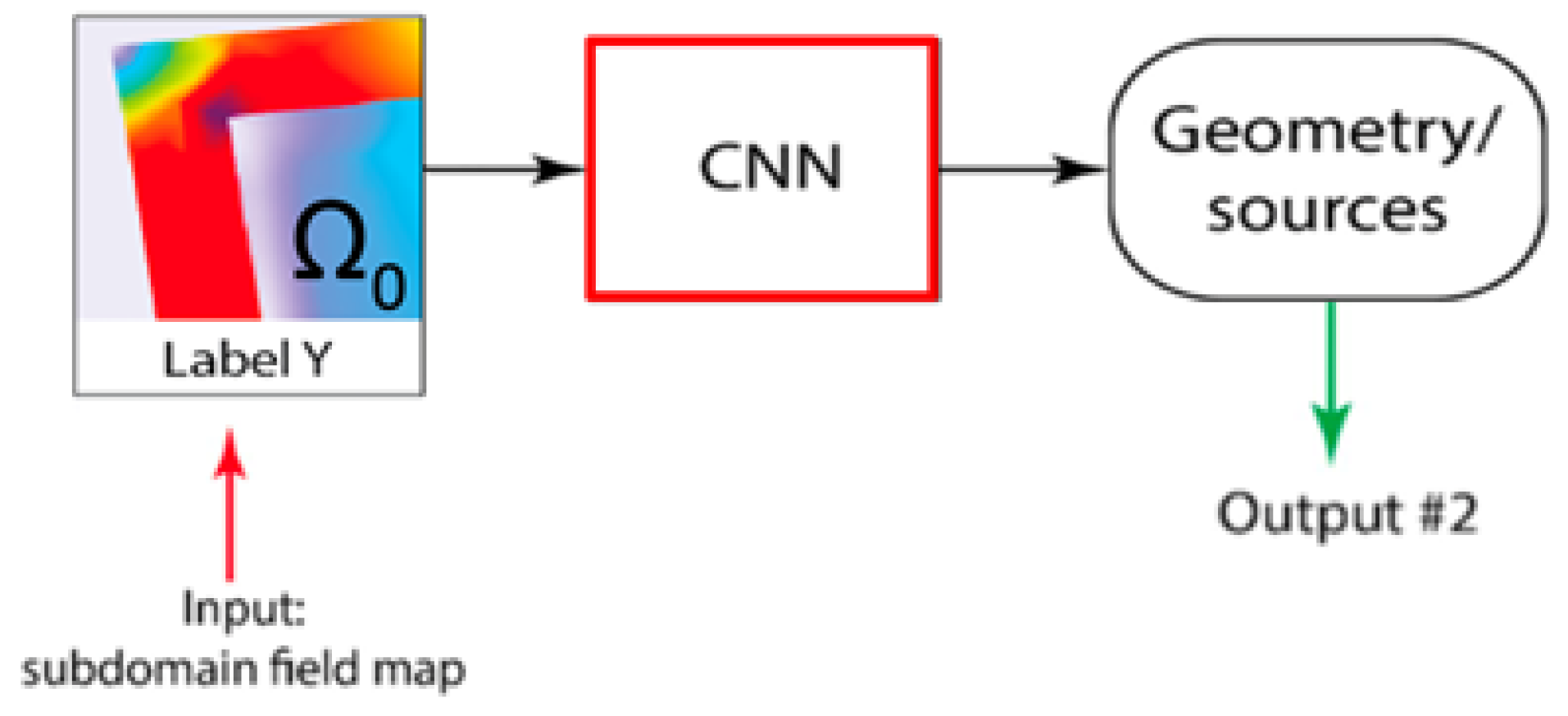
2.2.3. Approach 3: Convolutional Neural Network

The third approach is the most straightforward one, and it is represented in detail in Figure 4. In this case, there is no use of the CVAE, and the CNN works on the field data in the specific region of space Ω₀. As in approach 2, Output #1 (the reconstructed field) is not obtained, but there is no computational expense devoted to the training of the CVAE.

3. Case Study Description

As a benchmark magnetostatic problem, the authors considered the TEAM 35 problem [16,17] consisting in a small solenoid, e.g., for in vitro experiments of biomagnetism, in which the source of the magnetic field is a winding with a rectangular cross section (width $w=1$ mm, height $h=1.5$ mm) composed of 20 series-connected circular turns, each of them carrying DC current $I=3$ A (i.e., current density $J=2$ Amm⁻²), as shown in Figure 5.

The advantage of using a known problem, selected as a benchmark by the Compumag Society, lies in the fact that many solutions (obtained using completely different approaches) already exist, and will also be available and published in the future.

Due to its well-defined nature and manageable complexity, this problem could be effectively used by the authors both as a direct problem and as an inverse problem. Moreover, the initial problem formulation inherently includes a designated subregion (referred to as the Region of Interest, ROI, in [16,17]) where field optimization is required. This aspect led the authors to obviously consider the ROI as the subdomain Ω₀ where the field is considered known before the inversion.

The generation of the database is a two-step procedure; first a set of simulations performed using a Finite Element (FE) model are carried out, in order to find the magnetic field map for any physical configuration (direct problem). Consequently, the obtained field maps are post-processed with the goal of obtaining images that can be properly and efficiently managed by the DL algorithm (image processing).

3.1. Database Generation: Direct Problem Description

A Finite Element (FE) model was implemented, where only 10 turns were simulated, each characterized by radii $R_1,\cdots ,R_{10}$, respectively, and their variation range was $5\le R_i\le 50$ mm. A symmetric distribution of the radii was assumed with respect to the plane $z=0$. The geometry and a field map obtained using the FE model, implemented in Simcenter Magnet [19], are shown in Figure 5. In detail, the axisymmetric model is characterized by a rotational axis positioned at r = 0, while a symmetry condition was imposed at $z=0$. In this way, only 10 turns out of 20 were simulated. A vector potential formulation was implemented, and the complete domain measured 150 × 100 mm, and at $r=150\mathrm{m}\mathrm{m}$ and $z=100\mathrm{m}\mathrm{m}$, a tangential field was imposed. A triangular mesh, composed of roughly 55,000 s-order elements, was created using the vector potential formulation.

The whole domain Ω used for the DL-based approaches was a subset of the FE domain described before, and the sub-domain Ω₀ ⊂ Ω (where the fields are supposedly known in the inversion problems) is shown in Figure 5. The inverse problem can be formulated as follows: given the magnetic field distribution in the sub-domain Ω₀, identify the values of the radii of the ten turns. No assumptions on the location of the turns, which can belong to either Ω₀ or to Ω\Ω₀, were made. This problem was solved in three different ways, as described before: in Approach 1, the field reconstruction problem is solved for the domain Ω and then, based on the results of the first step, the identification problem of the coil geometry is solved for. In Approach 2 and Approach 3, the reconstruction of the field in Ω is not obtained and only the coil geometry is solved for.

The selection of the geometries can either follow some pre-defined guideline or can be completely random. At this stage of the research, where the main goal is to quantitatively evaluate and compare the performance of the methods, a set of geometries with given characteristics, which are described in the following order to guarantee repeatability, was the best choice. For this reason, three different geometries were considered, as reported in [13]:

• G1: turns with the same radius (solenoid-like geometry).
• G2: turns with an increasing radius along z (Δr = 1 mm).
• G3: turns with a decreasing radius along z (Δr = 1 mm).

This choice led to obtaining 451 solutions for geometry G1, 361 solutions for geometry G2, and 361 solutions for geometry G3.

3.2. Database Generation: Image Processing

Since the original FEM images are oversized for their direct use in DL methods (1000 × 1500 pixels), to make them suitable, they were initially cropped to focus on the variable radius region. However, even after the cropping, the images remained excessively large (225 × 550 pixels). Consequently, a resizing to 32 × 84 pixels was performed. Additionally, the subdomain image, extracted post-cropping, was also resized to the same dimensions of 32 × 84 pixels (Figure 6). This resizing aligns with the requirements of a DL approach that can be effectively trained using our available hardware. A global database of 1173 solutions was created. The training set contained 75%, i.e., 880, of the solutions, while the test set contained 25%, i.e., 293, of the solutions.

3.3. Metric Definitions for the Comparison between the Approaches

The common result of all methods is the so-called Output #2, i.e., the source geometry expressed as the radius of each coil. To evaluate the models, three metrics were used, the mean absolute percentage error (MAPE), the normalized root mean square error (NRMSE), and the normalized mean absolute error (NMAE), described in Equations (4)–(6), respectively:

$$MAPE=100\frac{1}{N_t}{\sum }_{N_t}\left|\frac{R_{pred}-R_{true}}{R_{true}}\right|$$

(4)

$$NRMSE=100\frac{\sqrt{\frac{1}{N_t}\sum _{N_t}{\left(R_{pred}-R_{true}\right)}^2}}{\sqrt{\frac{1}{N_t}\sum _{N_t}{\left(R_{true}\right)}^2}}$$

(5)

$$NMAE=100\frac{\frac{1}{N_t}\sum _{N_t}‖R_{pred}-R_{true}‖}{\max \left(R_{true}\right)-\min \left(R_{true}\right)}$$

(6)

where $N_t$ is the number of samples in the test set, and $R_{pred}$ and $R_{true}$ are the predicted and actual values of the radii, respectively.

These three metrics are known to have different sensitivities to large errors, which tend to have a greater effect on the NRMSE with respect to the MAPE and NMAE. Both the NRMSE and NMAE are alternative metrics that overcome the limitations of the more classical mean absolute percentage error in situations involving data that can be negative or close to zero, providing more balanced measures of accuracy.

4. Results

4.1. Approach 1: CVAE + CNN

The architectures of all the components of Approach 1 are reported in

Table 1. Encoder architecture ($213\times {10}^3$ learnables).

Layers	Activations
Image-based input (size 30 × 84) & Label (size 30 × 84)	30 × 84 × 2
2D Convolution (size 6 × 16, padd. same, stride 1)	30 × 84 × 16
Batch Norm.	30 × 84 × 16
ReLU act. fun.	30 × 84 × 16
Max Pooling 2D (stride 2 × 2)	15 × 42 × 16
2D Convolution (size 3 × 32, padd. same, stride 1)	15 × 42 × 32
Batch Norm.	15 × 42 × 32
ReLU act. fun.	15 × 42 × 32
Max Pooling 2D (stride 2 × 2)	7 × 21 × 32
2D Convolution (size 3 × 64, padd. same, stride 1)	7 × 21 × 64
Batch Norm.	7 × 21 × 64
ReLU act. fun.	7 × 21 × 64
Fully connected layer (20 outputs)	20 × 1

,

Table 2. Decoder architecture (${10}^7$ learnables).

Layers	Activations
Image-based input (size 1 × 1 × 10) & Labels (size 1 × 1 × 2520)	1 × 1 × 2530
Transp. Conv. 2D (size 3 × 420, stride 2 × 3, cropp. same)	2 × 3 × 420
ReLU act. fun.	2 × 3 × 420
Transp. Conv. 2D (size 5 × 35, stride 3 × 4, cropp. same)	6 × 12 × 35
ReLU act. fun.	6 × 12 × 35
Transp. Conv. 2D (size 10 × 16, stride 5 × 7, cropp. same)	30 × 84 × 16
ReLU act. fun.	30 × 84 × 16
Transp. Conv. 2D (size 3 × 8, stride 1 × 1, cropp. same)	30 × 84 × 8
ReLU act. fun.	30 × 84 × 16
Transp. Conv. 2D (size 3 × 1, stride 1 × 1, cropp. same)	30 × 84 × 1

and

Table 3. CNN architecture of approach 1 ($105\times {10}^3$ learnables).

Layers	Activations
Image-based input (size 30 × 84)	30 × 84 × 1
2D Convolution (size 3 × 8, padd. same, stride 1)	30 × 84 × 8
Batch Norm.	30 × 84 × 8
ReLU act. fun.	30 × 84 × 8
Aver. Pool. 2D (stride 2 × 2)	15 × 42 × 8
2D Convolution (size 3 × 16, padd. same, stride 1)	15 × 42 × 16
Batch Norm.	15 × 42 × 16
ReLU act. fun.	15 × 42 × 16
Aver. Pool. 2D (stride 2 × 2)	7 × 21 × 16
2D Convolution (size 3 × 32, padd. same, stride 1)	7 × 21 × 32
Batch Norm.	7 × 21 × 32
ReLU act. fun.	7 × 21 × 32
Aver. Pool. 2D (stride 2 × 2)	3 × 10 × 32
2D Convolution (size 3 × 64, padd. same, stride 1)	3 × 10 × 64
Batch Norm.	3 × 10 × 64
ReLU act. fun.	3 × 10 × 64
Aver. Pool. 2D (stride 2 × 2)	1 × 5 × 64
2D Convolution (size 3 × 128, padd. same, stride 1)	1 × 5 × 128
Batch Norm.	1 × 5 × 128
ReLU act. fun.	1 × 5 × 128
Dropout (20% probability)	1 × 5 × 128
Fully connected layer (10 outputs)	1 × 1 × 10
Regression layer	1 × 1 × 10

. The high number of learnable elements shows the complexity of the approach, which allows not only the calculation of the source geometry, but also the reconstruction of the field.

As is common in the cases of large deep neural networks, the choices of the architecture and hyperparameters of the CVAE and CNN are made heuristically by trial and error. The best performance of the CVAE was obtained by means of the following training options of the custom training loop: a minibatch size equal to 220, a number of epochs equal to 1000, a global learning rate of 10⁻³, a gradient decay factor of 0.9, and a squared gradient decay factor of 0.99. While for the CNN, the following values were found: a minibatch size equal to 32, a number of epochs equal to 800, an initial learning rate of 10⁻⁴, a learning rate drop factor of 0.9, and a learning rate drop period of 20. The method utilized for both the CVAE and the CNN training was Adaptive Moment Estimation (ADAM).

Following an 8 h training of the CVAE and 1 h training of the CNN, the results obtained for both the reconstruction and source identification are reported in

Table 4. Results obtained with Approach 1: CVAE.

Metric	Output #1 Reconstructed Field	Output #2 10 Radii
MAPE	4.24%	3.30%
NRMSE	4.14%	3.18%
NMAE	1.70%.	1.27%

: the mean percentage error for reconstructing the entire field map hovers around 4%, while identifying the 10 radii incurs an approximately 3% error. It is important to highlight again that the CNN receives as input the reconstructed field map.

4.2. Approach 2: Encoder + ANN

The encoder is the one described in Table 1, while the ANN is a fully connected network with two hidden sigmoidal layers of size 10. The time employed to train the CVAE is the same as before (even though the decoder is not used during the prediction phase in Approach 2), while the time needed to train the ANN was 10 min, using an early stop criterion based on the performance on a validation set. The results relative to the errors during the radius identification are reported in

Table 5. Results obtained with Approach 2: Encoder + ANN.

Metric	Output #1 Reconstructed Field	Output #2 10 Radii
MAPE	N.A.	2.28%
NRMSE	N.A.	1.98%
NMAE	N.A.	0.78%

, showing a performance around a 2% MAPE, while the performances for the field reconstruction are, of course, not available. The scatter plot shown in Figure 7 shows that in this approach, the true geometry was “missed” only three times.

4.3. Approach 3: CNN

The CNN architecture is shown in

Table 6. CNN architecture of approach 3 $(105\times {10}^3$ learnables).

Layers	Activations
Image-based input (size 30 × 84)	30 × 84 × 1
2D Convolution (size 3 × 8, padd. same, stride 1)	30 × 84 × 8
Batch Norm.	30 × 84 × 8
ReLU act. fun.	30 × 84 × 8
Aver. Pool. 2D (stride 2 × 2, stride 2)	15 × 42 × 8
2D Convolution (size 3 × 16, padd. same, stride 1)	15 × 42 × 16
Batch Norm.	15 × 42 × 16
ReLU act. fun.	15 × 42 × 16
Aver. Pool. 2D (2 × 2, stride 2)	7 × 21 × 16
2D Convolution (size 3 × 32, padd. same, stride 1)	7 × 21 × 32
Batch Norm.	7 × 21 × 32
ReLU act. fun.	7 × 21 × 32
Aver. Pool. 2D (2 × 2, stride 2)	3 × 10 × 32
2D Convolution (size 3 × 64, padd. same, stride 1)	3 × 10 × 64
Batch Norm.	3 × 10 × 64
ReLU act. fun.	3 × 10 × 64
Aver. Pool. 2D (2 × 2, stride 2)	1 × 5 × 64
2D Convolution (size 3 × 128, padd. same, stride 1)	1 × 5 × 128
Batch Norm.	1 × 5 × 128
ReLU act. fun.	1 × 5 × 128
Dropout (30% probability)	1 × 5 × 128
Fully connected layer (10 outputs)	1 × 1 × 10
Regression layer	1 × 1 × 10

, and it was directly trained on the field data in the subdomain Ω₀. It is worth it to note that the CNN architecture chosen for solving this problem is the same as the one used in Approach 1, but in order to achieve a better performance, in this CNN, the dropout probability was increased to 30%.

The best performance of the CNN was obtained with the following training options: a minibatch size equal to 64, a number of epochs equal to 1500, an initial learning rate of 10⁻⁴, a learning rate drop factor of 0.9, and a learning rate drop period of 20. The ADAM method was utilized for the CNN training; the resulting training time was 1 h.

The results relative to the errors during the radius identification are reported in

Table 7. Results obtained with Approach 3: CNN.

Metric	Output #1 Reconstructed Field	Output #2 10 Radii
MAPE	N.A.	2.54%
NRMSE	N.A.	3.28%
NMAE	N.A.	1.28%

, showing a MAPE performance between 2.5% and 3.5%; the performances for the field reconstruction are, of course, not present. The scatter plot shown in Figure 8 demonstrates that in this approach, the true geometry was “missed” several times in cases of geometry with large radii, i.e., far from the subdomain from which the image was provided as input to the CNN.

5. Discussion and Conclusions

In the context of deep learning, the so called “hold out” was the most common approach for validation, which consists of splitting the dataset into training and test sets and using the test data to compare and to assess the generalization capabilities of the models. In our case, the dataset was split into 75–25% training and testing, respectively. All performance results presented refer to the test errors. Regarding the selection of the hyper-parameters, due to the complexity of the deep learning models, a commonly used trial-and-error heuristic approach was adopted.

The training of the CVAE was performed using GPU computing, in particular, on an NVIDIA Quadro 4000 RTX, while the other neural networks were trained using parallel computing on a CPU, in particular, an AMD Zen 3 with 16 cores (32 threads). The software environment used was MATLAB 2022.

The cost of inference was negligible with all the models (below 300 ms), while the time required to carry out the optimization of the initial Z value at inference time was of the order of 10 s.

An overview of the performances of the three approaches can be obtained by analyzing and comparing Table 4, Table 5 and Table 7.

Approach 2 stands out as the most effective method for predicting the radii, utilizing the encoder’s latent space in conjunction with the CVAE. This fusion of an autoencoder and a fully connected NN enforces the effect of the CVAE’s regularization capabilities. While Approaches 1 and 3 show similarities in predicting the radii, Approach 1’s additional feature of reconstructing the entire field map makes it more comprehensive.

In addition, Approach 2 effectively handles the task of accurately predicting the correct geometry among the three options. The model misidentified the geometry only three times in the test set solutions. By replacing the autoencoder with a CNN (Approach 3), there is a slight dip in predicting the radii and a worsened normalized root mean square error (NRMSE). This performance decrease suggests that larger errors, impacting the NRMSE, arise from the CNN’s misjudgments, particularly for larger radii.

As far as the radii identification problem is concerned, in order to compare our approaches with a FEA and PDE-constrained optimizations the following remarks can be put forward. Referring to ref. [17], which shows different solutions of the TEAM 35 problem used as a test case in this paper, the costs of training and inference can be compared with the cost of conducting PDE-constrained optimization for an inverse design as follows. In view of a fair comparison, the lowest costs from Table 4 in [17], i.e., the cost of NSGA-II optimization, on a very similar problem, are considered: the optimization run for 100 iterations with a population of 20 individuals. This means that roughly 2000 FEAs for the whole optimization procedure are needed. Moreover, in the case of Cuckoo Search, the cost is approximately 200 iterations times 20 individuals, i.e., 4000 FEAs. On the other hand, the computational burden for training our networks is roughly 1200 FEAs.

It is worth it to notice that the optimizations carried out in [17] are general because 10 variables were considered as fully independent, while the approach proposed here is based on the parametrization of three families of geometries (G₁, G₂, and G₃) with a loss of generality. However, the cost of the optimization is firmly linked to a prescribed field distribution, and there is no flexibility, i.e., in changing the prescription, another optimization problem must be solved. In contrast, for any given field distribution in the subdomain, the same networks with no extra costs can be utilized—at least in principle—for solving the radius identification problem; and this is clearly an advantage.

To sum up, different deep learning approaches have been implemented and compared for solving inverse problems in the frame of TEAM benchmark problem 35. The CVAE approach can solve both inverse problems (field map reconstruction and radius identification) with good accuracy, but the CVAE structure is complex, and the training requires a long time. Both an ANN and CNN can solve the radius identification problem. The ANN approach applied to the latent space, however, requires CVAE training, but it shows a better accuracy with respect to the CNN and the CVAE itself. In using the latent space of a CVAE for the feature vectors, it seems that the more standard CNN approach can be outperformed.

References

1. Jin, Z.; Cao, Y.; Li, S.; Ying, W.; Krishnamurthy, M. Analytical Approach for Sharp Corner Reconstruction in the Kernel Free Boundary Integral Method during Magnetostatic Analysis for Inductor Design. Energies 2023, 16, 5420. [Google Scholar] [CrossRef]
2. Liebsch, M.; Russenschuck, S.; Kurz, S. BEM-based magnetic field reconstruction by ensemble Kálmán filtering. Comput. Methods Appl. Math. 2023, 23, 405–424. [Google Scholar] [CrossRef]
3. Formisano, A.; Martone, R. Different regularization methods for an inverse magnetostatic problem. Int. J. Appl. Electromagn. Mech. 2019, 60, S49–S62. [Google Scholar] [CrossRef]
4. Khan, A.; Ghorbanian, V.; Lowther, D. Deep Learning for Magnetic Field Estimation. IEEE Trans. Magn. 2019, 55, 7202304. [Google Scholar] [CrossRef]
5. Sasaki, H.; Igarashi, H. Topology Optimization Accelerated by Deep Learning. IEEE Trans. Magn. 2019, 55, 7401305. [Google Scholar] [CrossRef]
6. Pollok, S.; Bjørk, R.; Jørgensen, P.S. Inverse Design of Magnetic Fields Using Deep Learning. IEEE Trans. Magn. 2021, 57, 2101604. [Google Scholar] [CrossRef]
7. Amjad, J.; Lyu, Z.; Rodrigues, M.R.D. Deep Learning Model-Aware Regulatization with Applications to Inverse Problems. IEEE Trans. Signal Process. 2021, 69, 6371–6385. [Google Scholar] [CrossRef]
8. Jin, K.H.; McCann, M.T.; Froustey, E.; Unser, M. Deep convolutional neural network for inverse problems in imaging. IEEE Trans. Image Process. 2017, 26, 4509–4522. [Google Scholar] [CrossRef] [PubMed]
9. Liang, D.; Cheng, J.; Ke, Z.; Ying, L. Deep Magnetic Resonance Image Reconstruction: Inverse Problems Meet Neural Networks. IEEE Signal Process. Mag. 2020, 37, 141–151. [Google Scholar] [CrossRef] [PubMed]
10. Ongie, G.; Jalal, A.; Metzler, C.A.; Baraniuk, R.G.; Dimakis, A.G.; Willett, R. Deep Learning Techniques for Inverse Problems in Imaging. IEEE J. Sel. Areas Inf. Theory 2020, 1, 39–56. [Google Scholar] [CrossRef]
11. Goodfellow, I.; Bengio, Y.; Courville, A. Deep Learning; MIT Press: Cambridge, MA, USA, 2016. [Google Scholar]
12. Kingma, D.P.; Welling, M. An introduction to variational autoencoders. Found. Trends® Mach. Learn. 2019, 12, 307–392. [Google Scholar] [CrossRef]
13. Barmada, S.; Di Barba, P.; Fontana, N.; Mognaschi, M.E.; Tucci, M. Electromagnetic Field Reconstruction and Source Identification Using Conditional Variational Autoencoder and CNN. IEEE J. Multiscale Multiphys. Comput. Tech. 2023, 8, 322–331. [Google Scholar] [CrossRef]
14. Hall, P. On Kullback-Leibler loss and density estimation. Ann. Stat. 1987, 15, 1491–1519. [Google Scholar] [CrossRef]
15. Kingma, D.P.; Mohamed, S.; Jimenez Rezende, D.; Welling, M. Semi-supervised learning with deep generative models. In Proceedings of the Advances in Neural Information Processing Systems 27 (NIPS 2014), Cambridge, MA, USA, 8–13 December 2014; Volume 27. [Google Scholar]
16. Di Barba, P.; Mognaschi, M.E.; Lowther, D.A.; Sykulski, J.K. A Benchmark TEAM Problem for Multi-Objective Pareto Optimization of Electromagnetic Devices. IEEE Trans. Magn. 2018, 54, 9400604. [Google Scholar] [CrossRef]
17. Di Barba, P.; Mognaschi, M.E.; Lowther, D.A.; Sykulski, J.K. Improved solutions to a TEAM problem for multi-objective optimisation in magnetics. IET Sci. Meas. Technol. 2020, 14, 964–968. [Google Scholar] [CrossRef]
18. Fletcher, R. On the Barzilai–Borwein Method. In Optimization and Control with Applications; Applied Optimization; Qi, L., Teo, K., Yang, X., Eds.; Springer: Boston, MA, USA, 2005; Volume 96, pp. 235–256. [Google Scholar]
19. Siemens, Simcenter Magnet® Version 2022. Available online: https://www.plm.automation.siemens.com/global/it/products/simcenter/magnet.html (accessed on 1 January 2023).
Figure 1. Architectures of the three deep learning approaches: CVAE + CNN, Encoder + ANN, and CNN.
Mathematics 12 00859 g001
Figure 2. Architecture of Approach 1: CVAE + CNN.
Mathematics 12 00859 g002
Figure 3. Architecture of Approach 2: Encoder + ANN.
Mathematics 12 00859 g003
Figure 4. Architecture of Approach 3: CNN.
Mathematics 12 00859 g004
Figure 5. Magnetic induction B map with subdomains and radii highlighted.
Mathematics 12 00859 g005
Figure 6. Database generation: image processing.
Mathematics 12 00859 g006
Figure 7. Geometry prediction, Approach 2.
Mathematics 12 00859 g007
Figure 8. Geometry prediction, Approach 3.
Mathematics 12 00859 g008