Element Aggregation for Estimation of High-Dimensional Covariance Matrices

Abstract

This study addresses the challenge of estimating high-dimensional covariance matrices in financial markets, where traditional sparsity assumptions often fail due to the interdependence of stock returns across sectors. We present an innovative element-aggregation method that aggregates matrix entries to estimate covariance matrices. This method is designed to be applicable to both sparse and non-sparse matrices, transcending the limitations of sparsity-based approaches. The computational simplicity of the method’s implementation ensures low complexity, making it a practical tool for real-world applications. Theoretical analysis then confirms the method’s consistency and effectiveness with its convergence rate in specific scenarios. Additionally, numerical experiments validate the method’s superior algorithmic performance compared to conventional methods, as well as the reduction in relative estimation errors. Furthermore, empirical studies in financial portfolio optimization demonstrate the method’s significant risk management benefits, particularly its ability to effectively mitigate portfolio risk even with limited sample sizes.

1. Introduction

Covariance matrix estimation is essential in statistics [1], econometrics [2], finance [3], genomic studies [4], and other related fields. This matrix quantifies the pairwise interdependencies between variables in a dataset, and each element signifies the covariance between two variables. The accuracy of this estimation is critical for statistical and data analyses. As the size of the matrix increases, the efficiency of the estimation process often decreases. Therefore, the development of efficient methods for this estimation remains a significant research challenge. Various approaches concentrate on assuming specific features in the matrix. Initial methods include principal component analysis (PCA) [5] and factor models [6]. Other prevalent techniques encompass the constant correlation approach [7], maximum likelihood estimation (MLE) [8], shrinkage methods [9,10], and so on [11]. Notably, shrinkage methods have demonstrated exceptional efficacy in financial portfolio allocation.

For the estimation of sparse or approximately sparse covariance matrices, various element-wise thresholding techniques for the sample covariance matrix have emerged. These include hard thresholding [12,13], soft thresholding with extensions [14], and adaptive thresholding [15,16]. Generally, these methods offer low computational demands and high consistency. However, the resulting matrix might not always be semi-positive definite. To address this, more sophisticated methods have been introduced to ensure the estimators are semi-positive definite [17,18].

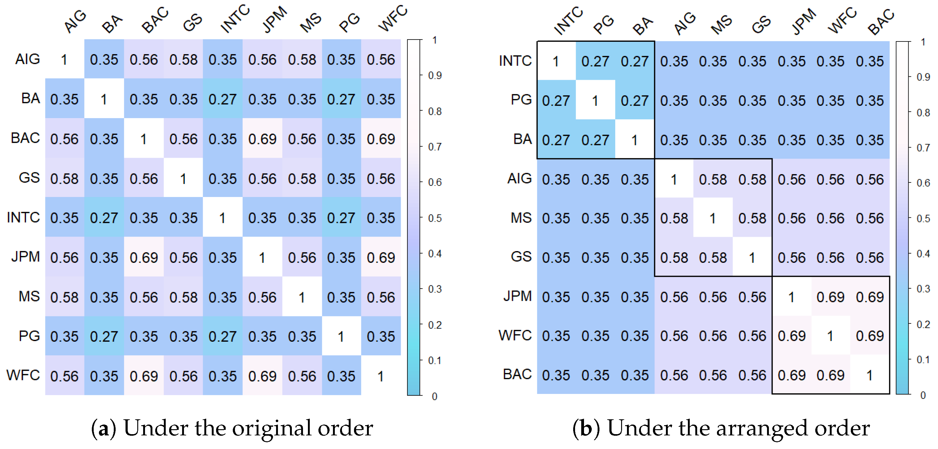
While the sparsity condition is often assumed in [6,19], it is not universally applicable. For instance, in financial studies, variables such as stock returns often share common factors, making the sparsity assumption less appropriate. Instead, a more common pattern in the covariance matrix of financial data is the clustering of entries. This occurs because stocks within the same industry sector are often similarly correlated with stocks from other sectors [20]. An illustrative example is provided by [21,22], who analyzed the daily returns of nine companies on the New York Stock Exchange (NYSE) market based on 2515 observations from 2000 to 2009. Their analysis revealed a matrix of correlation coefficients without zero entries, with many coefficients sharing identical values. Using statistical hypothesis testing, the correlation coefficients were grouped into five distinct values $(0.27,0.35,0.56,0.58,0.69)$, shown in Figure 1a. A similar observation was made by [23]. When stocks are arranged in a particular order, the correlation coefficient matrix manifests itself as a block-symmetric matrix, as depicted in Figure 1b, which can be written as

$$\left(\begin{array}{ccc}1-0.27& 0& 0\\ 0& 1-0.58& 0\\ 0& 0& 1-0.69\end{array}\right)\otimes I_3+\left(\begin{array}{ccc}0.27& 0.35& 0.35\\ 0.35& 0.58& 0.56\\ 0.35& 0.56& 0.69\end{array}\right)\otimes \left(\begin{array}{ccc}1& 1& 1\\ 1& 1& 1\\ 1& 1& 1\end{array}\right),$$

where ⊗ is the Kronecker product. We will demonstrate later that this uncomplicated framework is highly effective for estimating the covariance matrix in Corollary 3.

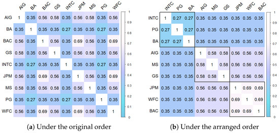
Figure 1. Correlation coefficient matrix of the daily returns of 9 companies with stock symbols AIG, BA, BAC, GS, INTC, JPM, MS, PG, and WFC on the NYSE market.

The proposed estimation method in this paper derives from the correlation matrix structure mentioned earlier. This structure is widespread in numerous financial research situations, encompassing sparse covariance matrices, the formerly noted block-wise covariance matrices, and all correlation coefficients in a global constant [24]. However, many existing methods are unsuitable for estimating covariance matrices under this structure. To broaden our scope, we delve into the estimation of covariance matrices with clustered entries. To achieve this, we propose an element-aggregation method that is tailored towards covariance matrix estimation. Moreover, we examine the theoretical properties of our method and confirm its effectiveness through extensive numerical simulations and real-world data analysis.

The rest of this paper is organized as follows. In Section 2, we propose the element-aggregation method for covariance matrix estimation while also elucidating its implementation. Section 3 assesses the theoretical consistency of the estimation errors and exhibits corresponding convergence rates. All theoretical proofs are in Appendix A, Appendix B, Appendix C, Appendix D, Appendix E and Appendix F. Numerical simulation analyses and real data analysis with portfolio allocation are presented in Section 4 and Section 5, respectively. Conclusions are provided in Section 6.

2. Estimation and Implementation for Covariance Matrix

Suppose the multiple random variable $X={({\mathbf{x}}_1,\dots ,{\mathbf{x}}_p)}^{\top }$ has the covariance matrix $\mathrm{\Sigma }={\left({\sigma }_{ij}\right)}_{1\le i,j\le p}$, and samples $X_i={(x_{i1},\dots ,x_{ip})}^{\top }$, $i=1,\dots ,n$ are generated from X. The sample covariance matrix is defined as $\widehat{\mathrm{\Sigma }}={\left({\widehat{\sigma }}_{ij}\right)}_{1\le i,j\le p}$. For $1\le i,j\le p$,

$${\widehat{\sigma }}_{ij}=n^{-1}\sum _{\mathsf{\ell }=1}^n{\pi }_{\mathsf{\ell },ij},$$

where ${\pi }_{\mathsf{\ell },ij}=(x_{\mathsf{\ell }i}-{\overline{x}}_i)(x_{\mathsf{\ell }j}-{\overline{x}}_j)$ and ${\overline{x}}_k=n^{-1}{\sum }_{\mathsf{\ell }=1}^n{x}_{\mathsf{\ell }k}$ for $k=1,\dots ,p$.

Motivated by the structure of the correlation matrix discussed in the introduction and aiming to analyze the covariance matrices with clustered entries, we consider the following specification for the covariance matrix. Let $\mathrm{\Omega }=\{{\sigma }_{ij}:i<j\}$ denote the collection of off-diagonal elements in the covariance matrix $\mathrm{\Sigma }$, and let the set of distinct elements in $\mathrm{\Omega }$ be represented by

$$\aleph =\{{\varsigma }_k\in \mathrm{\Omega }:{\varsigma }_k\ne {\varsigma }_{k^{\prime }},\forall 1\le k\ne k^{\prime }\le K\},$$

where K is the cardinality of set ℵ, and K changes with p. In other words, ${\sigma }_{ij}\in \aleph$ for all $1\le i<j\le p$. For $k=1,\dots ,K$, the index set of covariance matrix elements that are equal to ${\varsigma }_k$ is defined as

$${\aleph }_k=\{(i,j):{\sigma }_{ij}={\varsigma }_k,1\le i<j\le p\}.$$

In brief, ${\aleph }_k$ stands for the category of ${\varsigma }_k$. Similarly, for $1\le i<j\le p$, the index set of covariance matrix elements that are equal to ${\sigma }_{ij}$ is defined as

$${\aleph }_{ij}=\{(a,b):{\sigma }_{ab}={\sigma }_{ij},1\le a<b\le p\}.$$

Then, for $(i,j)\in {\aleph }_k$, we have ${\aleph }_{ij}={\aleph }_k$.

If the sets ${\aleph }_k,k=1,\dots ,K$ are known, i.e., the indices for same elements in $\mathrm{\Sigma }$ are known, then we can estimate ${\varsigma }_k$ by averaging the sample covariance elements ${\widehat{\sigma }}_{ij}$ as follows for all $(i,j)\in {\aleph }_k$,

$$\begin{array}{cc}\hfill {\check{\varsigma }}_k=& \frac{1}{\#{\aleph }_k}\sum _{(i,j)\in {\aleph }_k}{\widehat{\sigma }}_{ij}\hfill \\ \hfill =& n^{-1}\frac{1}{\#{\aleph }_k}\sum _{\mathsf{\ell }=1}^n\sum _{(i,j)\in {\aleph }_k}{\pi }_{\mathsf{\ell },ij},\hfill \end{array}$$

(1)

where $\#{\aleph }_k$ is the cardinality of set ${\aleph }_k$. Thus, the covariance matrix $\mathrm{\Sigma }$ can be estimated by

$$\check{\mathrm{\Sigma }}=\left({\check{\sigma }}_{ij}\right),\mathrm{with}{\check{\sigma }}_{ij}={\check{\varsigma }}_k,\mathrm{if}(i,j)\in {\aleph }_k.$$

(2)

Element-Aggregation Estimation Method (ELA)

We hereby introduce the element-aggregation (ELA) estimation method for estimation purposes. As ${\aleph }_k$ is unknown, we estimate ${\aleph }_{ij}$, i.e., the category of each ${\sigma }_{ij}$, as follows,

$${\tilde{\aleph }}_{ij}=\{(a,b):|{\widehat{\sigma }}_{ij}-{\widehat{\sigma }}_{ab}|<c{\widehat{\varrho }}_{ij}\sqrt{\frac{log(p\vee n)}{n}},1\le a<b\le p\},$$

(3)

where ${\widehat{\varrho }}_{ij}$ is a sample estimate of ${\varrho }_{ij}=Var\left({\pi }_{ij}\right)$ and c is a tuning parameter. Regarding the choice of this tuning parameter c, Cai and Liu [15] show that a good choice of the tuning parameter c does not affect the rate of convergence but it does affect the numerical performance of the estimators. The tuning parameter c can be taken as fixed at $c=2$, as suggested in [15], or it can be chosen empirically by cross-validation, such as via the five-fold cross-validation method used in [12,15]. The tuning parameter c operates akin to a significance level in statistical testing, and the 2-$\sigma$ rule is widely endorsed for normally distributed data, wherein approximately $95\%$ of observations are encapsulated within the interval of the mean plus or minus two standard deviations, denoted as $[\mu -2\sigma ,\mu +2\sigma ]$. In our simulations, we also discover that employing $c=2$ as the tuning parameter for the proposed ELA algorithm yields commendable performance in high-dimensional cases, and does not differ significantly from the parameter optimization obtained by cross-validation. Consequently, we adopt $c=2$ as the tuning parameter for our subsequent analysis.

Analogous to (1), we estimate the covariance matrix element ${\sigma }_{ij}$ by

$${\tilde{\sigma }}_{ij}=n^{-1}\frac{1}{\#{\tilde{\aleph }}_{ij}}\sum _{\mathsf{\ell }=1}^n\sum _{(s,t)\in {\tilde{\aleph }}_{ij}}{\pi }_{\mathsf{\ell },st},$$

(4)

and $\mathrm{\Sigma }$ by $\tilde{\mathrm{\Sigma }}=\left({\tilde{\sigma }}_{ij}\right)$. This is the element-aggregation (ELA) estimator of the covariance matrix.

In terms of computational complexity, the ELA process requires $O(p^{2}log\left(p\right))$ time, where $log\left(p\right)$ accounts for the binary search computation of ${\tilde{\aleph }}_{ij}$ in $\{{\widehat{\sigma }}_{ab}:1\le a<b\le p\}$. In comparison, element-wise thresholding has a computational complexity of $O\left(p^2\right)$. Therefore, the ELA estimation calculation is only slightly more complex than the element-wise thresholding approach.

3. Theoretical Properties

In this section, we provide the theoretical justification for the element-aggregation estimation under the assumption of a normal distribution of X. The results can be proven under more general conditions using more complicated techniques. Let $\parallel A\parallel$ denote the operator norm, i.e., $\parallel A\parallel ={\left\{{\lambda }_{max}\left(A{A}^{\top }\right)\right\}}^{1/2}$, where ${\lambda }_{max}\left(A{A}^{\top }\right)$ is the square root of the largest eigenvalue of $A{A}^{\top }$.

Lemma 1. 

Let K be the number of different values of the off-diagonal elements in the covariance matrix $Cov\left(X\right)=\mathrm{\Sigma }$. Let $n_{i,k}$ be the numbers of elements that are equal to ${\varsigma }_k$ in the i-th row of Σ, i.e., $n_{i,k}=\#\{j:{\sigma }_{ij}={\varsigma }_k,1\le j\ne i\le p\}$. If $\underset{1\le i,j\le p}{max}{\sigma }_{ij}\le M_0$ for some constant $M_0$ and

$$Var\left(\frac{1}{\sqrt{\#{\aleph }_k}}\sum _{(i,j)\in {\aleph }_k}{\pi }_{\mathsf{\ell },ij}\right)=O\left(V_k^2\right),k=1,\dots ,K,$$

where $V_k=\mathrm{Var}\left({\check{\varsigma }}_k\right)$ and ${\check{\varsigma }}_k$ is the estimate in (1), then the covariance matrix estimator $\check{\mathrm{\Sigma }}$ in (2) has the following estimation error

$$\parallel \check{\mathrm{\Sigma }}-\mathrm{\Sigma }\parallel =O_P\left(\sqrt{\frac{log(p\vee n)}{n}}\right)\sum _{k=1}^K\frac{n_{j,k}}{\sqrt{\#{\aleph }_k}}{V}_k.$$

An important characteristic is that the effect of dimension on the estimation error is regulated by a slowly varying function, $log\left(p\right)$. Lemma 1 could also be extended to the case that ${\aleph }_k$ is unknown. In such cases, we need to identify the corresponding category ${\aleph }_k$. To simplify the explanation, we will use ${\aleph }_{ij}$ here, since ${\aleph }_{ij}={\aleph }_k$ if $(i,j)\in {\aleph }_k$.

Lemma 2. 

Suppose X is normally distributed with $\underset{1\le i,j\le p}{max}{\sigma }_{ij}\le M_0$ for some constant $M_0$. If

$$\sqrt{n}min\{|{\varsigma }_k-{\varsigma }_j|,k\ne j\}/{(log(p\vee n))}^{1/2}\to \infty ,$$

then the identification by (3) is consistent, i.e., for any $(i,j)\in {\aleph }_k$,

$$Pr(\bigcup _{1\le i,j\le p}\{{\tilde{\aleph }}_{ij}\ne {\aleph }_{ij}\})\to 0.$$

Theorem 1. 

With the above notation, if the conditions in Lemmas 1 and 2 are satisfied, then

$$\parallel \tilde{\mathrm{\Sigma }}-\mathrm{\Sigma }\parallel =O_P\left(\sqrt{\frac{log(p\vee n)}{n}}\right)\sum _{k=1}^K\frac{n_{j,k}}{\sqrt{\#{\aleph }_k}}{V}_k.$$

(5)

Below, we give some special cases of Theorem 1, and show the convergence rates in Corollaries 1–3.

Corollary 1. 

Suppose $\mathrm{\Sigma }={\left({\sigma }_{ij}\right)}_{1\le i,j\le p}$ is sparse with a number of non-zero elements in each row of $o\left(p\right)$, i.e., $c\left(p\right)/p\to 0$, where $c\left(p\right)={max}_j{\sum }_{i=1}^p({\sigma }_{ij}\ne 0)$. If the conditions in Theorem 1 hold, then

$$\parallel \tilde{\mathrm{\Sigma }}-\mathrm{\Sigma }\parallel =O_P\left(c\left(p\right)\sqrt{\frac{log(p\vee n)}{n}}\right).$$

This result is a special case in [12]. It could be extended to more general cases.

Corollary 2. 

Suppose $X={({\mathbf{x}}_1,\dots ,{\mathbf{x}}_p)}^{\top }$ follows normal distribution with $\mathrm{\Sigma }={\left({\varsigma }_{|i-j|}\right)}_{1\le i,j\le p}.$ If $|{\varsigma }_k|=O\left(c^k\right)$ for some $c<1$, then

$$\parallel \tilde{\mathrm{\Sigma }}-\mathrm{\Sigma }\parallel =O_P\left(log\left(p\right)\sqrt{\frac{log(p\vee n)}{n}}\right).$$

Finally, we consider a simple block covariance matrix with the matrix in Figure 1b as a special case.

Corollary 3. 

Suppose $\mathrm{\Sigma }={\mathrm{\Lambda }}_M\otimes I_m+{\mathrm{\Phi }}_M\otimes {\mathrm{\Xi }}_m$ where $I_m$ is a $m\times m$ identity matrix, ${\mathrm{\Lambda }}_M$ is a diagonal matrix, ${\mathrm{\Xi }}_m$ is a $m\times m$ matrix with all elements 1, and ${\mathrm{\Phi }}_M$ is an $M\times M$ symmetric matrix. If M is fixed as $p\to \infty$, then we have

$$||\tilde{\mathrm{\Sigma }}-\mathrm{\Sigma }||=O_P\left(n^{-1/2}\right).$$

Remark 1. 

Since the dimension M of the matrix ${\mathrm{\Phi }}_M$ and the diagonal matrix ${\mathrm{\Lambda }}_M$ assumed in Corollary 3 are fixed ($p\to \infty$), the different values for their matrix elements are at most $M(M+1)/2$ and M, respectively, so Σ also has at most $M(M+3)/2$ different values, which is fixed at $p\to \infty$. By Lemma 2, the estimates ${\tilde{\mathrm{\Lambda }}}_M$ and ${\tilde{\mathrm{\Phi }}}_M$ satisfy the rate of $O_P\left(n^{-1/2}\right)$, i.e., for any $\delta >0$, a subset of the probability space $S_n:Pr\left(S_n\right)>1-\delta$ can be found, such that

$$||{\tilde{\mathrm{\Lambda }}}_M-{\mathrm{\Lambda }}_M||=O_P\left(n^{-1/2}\right),||{\tilde{\mathrm{\Phi }}}_M-{\mathrm{\Phi }}_M||=O_P\left(n^{-1/2}\right).$$

where $\tilde{\mathrm{\Sigma }}={\tilde{\mathrm{\Lambda }}}_M\otimes I_m+{\tilde{\mathrm{\Phi }}}_M\otimes {\mathrm{\Xi }}_m.$ Using the eigenvalue and Kronecker product properties, we show in the Appendix A, Appendix B, Appendix C, Appendix D, Appendix E and Appendix F that the covariance matrix estimate $\tilde{\mathrm{\Sigma }}$ also has the same rate $O_P\left(n^{-1/2}\right)$. That is, since the number of selectable elements of the covariance matrix is determined by a fixed M, which is not dependent on p, the rate of convergence for the covariance matrix estimate $\tilde{\mathrm{\Sigma }}$ is also independent of p.

Our ELA method efficiently estimates the covariance matrix with the above structure, demonstrating both efficiency and dimensional independence. Mathematically, this block-wise structure is straightforward. Furthermore, we hypothesize that these conclusions can be extended to more general block-wise matrices, such as the Khatri–Rao product or the Tracy–Singh product [25].

4. Numerical Simulation

Our study presents the ELA method to estimate the covariance matrix using an element-aggregation idea. The ELA method is designed for simplicity and clarity, making it easy to implement. The steps for implementing the method were thoroughly detailed in the preceding section. This section focuses on comparing the algorithmic performance of the proposed method with several estimation methods for high-dimensional sparse and non-sparse covariance matrices. We compare our ELA estimation method with multiple established methods: (1) the adaptive thresholding method [15], (2) the POET_k method [19] with $k=0,1,2,\dots$ factors, and (3) the Rothman method [18].

The numerical simulation focuses on the relative matrix errors when estimating the covariance matrix and the correlation coefficient matrix. To estimate the covariance matrix, first standardize each variable. Then, multiply the elements of the correlation coefficient matrix by the sample standard deviations of each random variable. This effectively transforms the estimation of the covariance matrix into the estimation of the corresponding correlation coefficient matrix. Thus, the ELA method’s efficiency and accuracy in capturing the underlying data structure can be comprehensively assessed through the dual focus on both covariance and correlation coefficient matrix estimations.

The metric employed to compare the estimation efficiency between these estimation methods is the average matrix loss over 500 replications. The matrix losses are measured by the spectral norm of the correlation coefficient matrix and the covariance matrix, similar to that performed in [18]. To aid visualization, we define the relative estimation errors between the estimated matrix and the actual matrix for both the correlation coefficient matrix R and the covariance matrix $\mathrm{\Sigma }$ as follows:

$$e_{cor}=\frac{\parallel \widehat{R}-R\parallel }{\parallel R\parallel }\times 100\%,e_{cov}=\frac{\parallel \widehat{\mathrm{\Sigma }}-\mathrm{\Sigma }\parallel }{\parallel \mathrm{\Sigma }\parallel }\times 100\%.$$

where $\parallel A\parallel ={\left\{{\lambda }_{max}\left(A{A}^{\top }\right)\right\}}^{1/2}$ denote the operator norm. The next simulation compares the relative matrix estimation errors for various matrix types and algorithms, but also shows how the matrix estimation error changes as the matrix dimension p increases, in order to demonstrate more clearly the superiority of the proposed estimation algorithm.

The following three covariance matrices $\mathrm{\Sigma }={\left({\sigma }_{ij}\right)}_{1\le i,j\le p}$ are considered.

Example 1. 

${\sigma }_{ij}=\sqrt{ij}{\rho }^{|i-j|}$ with $\rho =-0.9$.

Example 2. 

${\sigma }_{ij}={\left(ij\right)}^{1/4}{r}_{ij}$ where $r_{ii}=1,r_{ij}=0.6{|i-j|}^{-1}{u}_{ij}$ for $i\ne j$ and $u_{ij}=u_{ji}$ are IID uniform on [0, 1]. A similar example was used in [16].

Example 3. 

Constant block matrix

$$\mathrm{\Sigma }=\left(\begin{array}{cc}{\mathrm{\Sigma }}_1& {\mathrm{\Sigma }}_2\\ {\mathrm{\Sigma }}_2& {\mathrm{\Sigma }}_3\end{array}\right)$$

where ${\mathrm{\Sigma }}_1=0.8{\mathrm{\Xi }}_{p/2}+0.2I_{p/2},{\mathrm{\Sigma }}_2=-0.4{\mathrm{\Xi }}_{p/2},{\mathrm{\Sigma }}_3=0.3{\mathrm{\Xi }}_{p/2}+0.7I_{p/2}$, ${\mathrm{\Xi }}_{p/2}$ is a $(p/2)\times (p/2)$ matrix with all elements 1, and $I_{p/2}$ is the identity matrix of size $p/2$.

Remark 2. 

Due to the assumption of sparse covariance matrices in the adaptive thresholding method, the POET₀ method, and the Rothman estimation method [6,15,18], the covariance matrix is estimated as a sparse matrix, where most of the matrix elements are estimated to be zero. This is significantly different from the non-sparse covariance matrix in Example 3. The relative estimation error of the covariance matrix estimated by these methods is relatively large compared to the sample covariance estimation method. Therefore, the adaptive thresholding method, the POET₀ method, and the Rothman method cannot be used directly for Example 3.

Note that Σ can be written as

$$\mathrm{\Sigma }={\mathrm{\Sigma }}_0+{\lambda }_1{\mathsf{\ell }}_1{\mathsf{\ell }}_1^{\top }+{\lambda }_2{\mathsf{\ell }}_2{\mathsf{\ell }}_2^{\top },$$

where ${\mathrm{\Sigma }}_0$ is a sparse matrix and ${\lambda }_1$ and ${\lambda }_2$ are the first two largest eigenvalues of Σ, with ${\mathsf{\ell }}_1$ and ${\mathsf{\ell }}_2$ as the corresponding eigenvectors, respectively. By this decomposition, the POET_k method with $k=2$ factors in [19] can be used, i.e., POET₂ is applicable to the estimation for Example 3.

Random samples are generated from $X\sim N(0,\mathrm{\Sigma })$ with sample sizes $n=(100,200)$ and $p=(100,500,900,1400,1900,2300,2500)$. The averages of the relative estimation errors, based on 500 replications, are depicted in Figure 2, Figure 3 and Figure 4. The ELA method is represented by a solid red line. Only methods with a performance comparable to the best one are displayed in each panel.

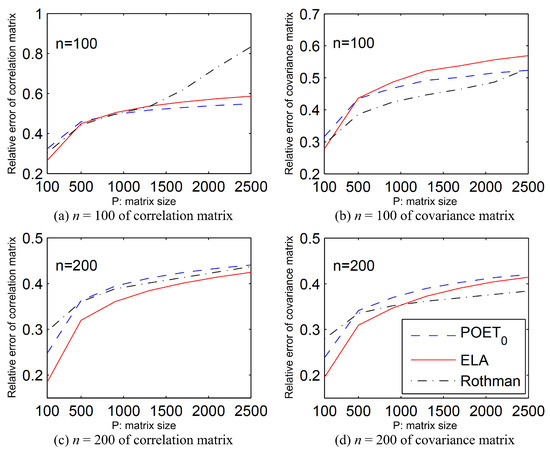
Figure 2. Relative estimation error for the correlation matrix (left) and the covariance matrix (right) in Example 1 with sample sizes $n=100$ and 200; the estimation is based on 500 replications per data point.

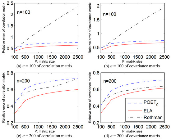
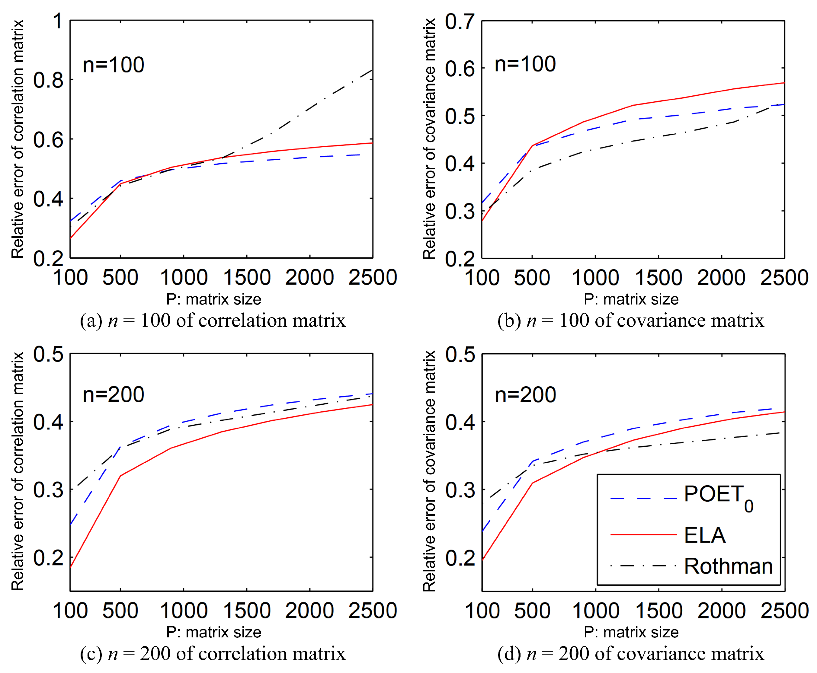
Figure 3. Relative estimation error for the correlation matrix (left) and the covariance matrix (right) in Example 2 with sample sizes $n=100$ and 200; the estimation is based on 500 replications per data point.

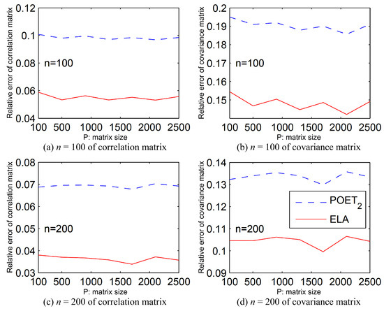
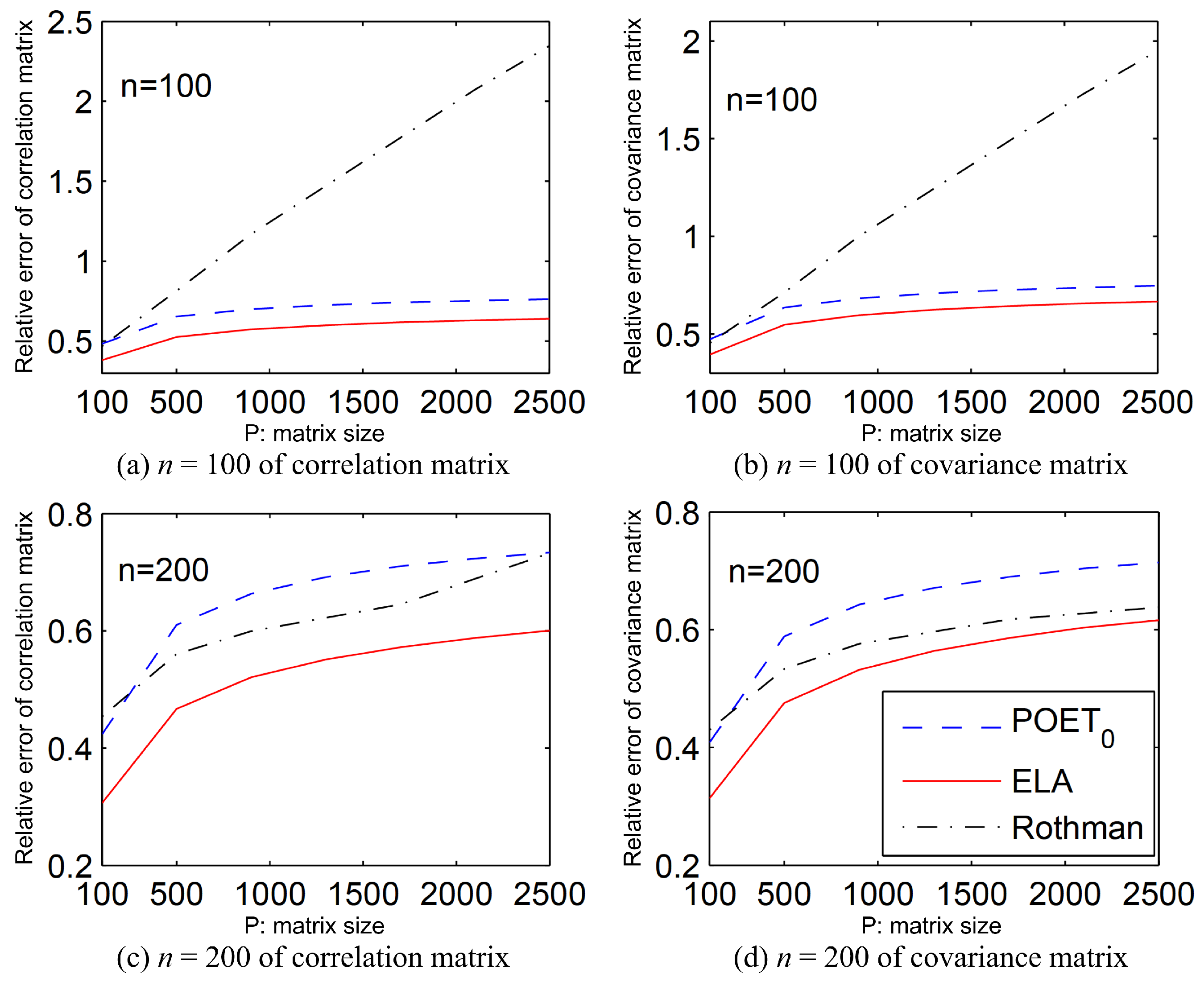
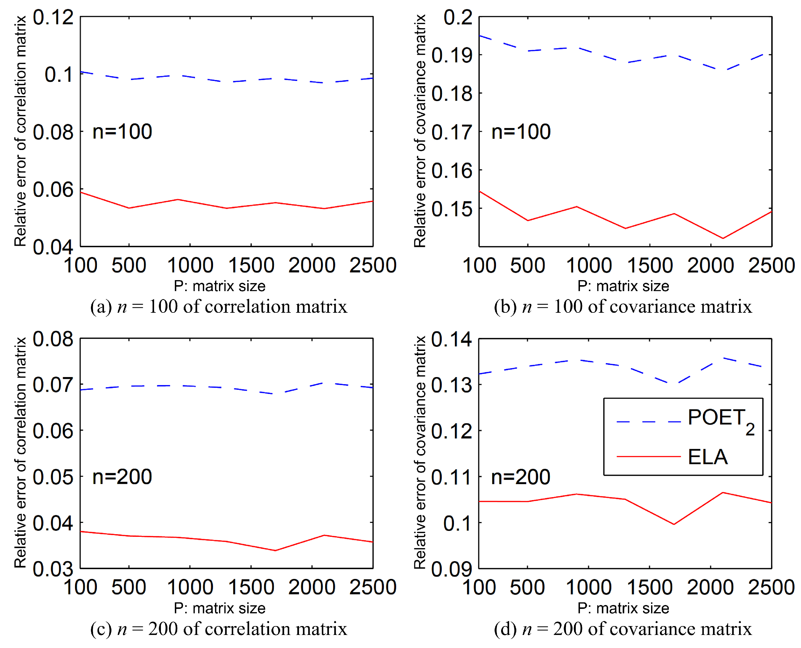
Figure 4. Relative estimation error for the correlation matrix (left) and the covariance matrix (right) in Example 3 with sample sizes $n=100$ and 200; the estimation is based on 500 replications per data point.

In Figure 2 for Example 1 with $n=100$, our ELA estimator for the correlation coefficient matrix R is slightly inferior to POET₀ but exceeds Rothman. For the covariance matrix $\mathrm{\Sigma }$, our method slightly lags behind both POET₀ and Rothman. However, with $n=200$, the ELA method outperforms them in both the correlation coefficient matrix and the covariance matrix with $p<1000$, ranking first for the correlation coefficient matrix and second for the covariance matrix with $p>1000$. In general, the ELA method is comparable to both POET and Rothman for Example 1.

In Figure 3 for Example 2, the ELA estimator consistently outperforms both POET and Rothman for both matrices when $n=(100,200)$. Although Remark 2 suggests that POET₂ is suitable for Example 3, Figure 4 for Example 3 demonstrates the superior efficiency of the ELA method over POET₂ for both matrices with $n=(100,200)$. In summary, the ELA method significantly outperforms both POET and Rothman for Examples 2 and 3.

Furthermore, we conducted a comprehensive analysis comparing the average computational time across 500 replications for our ELA method alongside the adaptive thresholding method [15], the POET method [19], and the Rothman method [18]. These comparisons are detailed in Table 1. The random samples are still generated from $X\sim N(0,\mathrm{\Sigma })$ with $\mathrm{\Sigma }$ following Example 1, sample sizes $n=(100,200)$, and covariance matrix dimensions $p=(100,500,900,1400,1900,2300,2500)$. Notably, due to the POET_k methods exhibiting computational times that are broadly analogous for different values of k, we present only the results for POET₁.

Table 1. The average computational time over 500 replications of the ELA method, the adaptive thresholding method, the POET₁ method, and the Rothman method for sample sizes $n=(100,200)$ and $p=(100,500,900,1400,1900,2300,2500)$ (in seconds).

Method	Adaptive Thresholding		POET		Rothman		ELA
$\mathit{p}$	$\mathit{n}=\mathbf{100}$	$\mathit{n}=\mathbf{200}$	$\mathit{n}=\mathbf{100}$	$\mathit{n}=\mathbf{200}$	$\mathit{n}=\mathbf{100}$	$\mathit{n}=\mathbf{200}$	$\mathit{n}=\mathbf{100}$	$\mathit{n}=\mathbf{200}$
100	0.005	0.006	0.222	0.815	0.012	0.013	0.034	0.037
500	0.370	0.409	0.806	2.042	0.828	0.830	0.863	0.930
900	2.176	2.207	2.657	5.163	4.680	4.910	2.849	3.131
1400	7.967	7.467	9.248	12.711	18.444	18.442	7.743	8.087
2300	44.901	43.974	34.241	42.228	81.292	81.834	20.525	23.054
2500	60.117	60.876	43.077	52.826	108.323	110.301	25.317	25.570

Upon examination of Table 1, it is evident that, for lower dimensions of $p=(100,500)$, the ELA method has a higher computational cost compared to the adaptive thresholding and Rothman methods but outperforms the POET method. For $p=(900,1400)$, the ELA method is slightly slower than adaptive thresholding but remains superior to both the POET and Rothman methods. When dealing with higher dimensions of $p=(2300,2500)$, the ELA method demonstrates a significant computational advantage over its counterparts. This suggests that the ELA method scales more efficiently with increasing dimensionality, which is a desirable attribute for high-dimensional data analysis.

Our simulation studies have yielded the following conclusions: The ELA method outperforms both POET and Rothman for Examples 2 and 3 in both the correlation coefficient matrix and the covariance matrix with $n=(100,200)$ and $p=(100,\dots ,2500)$. For Example 1, it performs comparably to them. These results emphasize the efficiency of the ELA method for estimating covariance matrices. Our proposed ELA technique is not just computationally efficient but also markedly lowers the relative estimation error, i.e., with minimal loss of spectral norm for the correlation coefficient and the covariance matrix.

5. Real Data Analysis and Portfolio Allocation

The component stocks of the SP500 index were analyzed using historical daily prices sourced from Yahoo Finance through the R package ‘tidyquant’. We selected 430 stocks from SP500 with daily prices spanning over 3000 days, from 1 January 2008 to 31 December 2019, to ensure a sufficiently large sample size. This allowed for a larger window, $N=500$, to be selected when we use the rolling window method later. Our emphasis is on the correlation coefficient matrix and covariance matrix for daily returns. Although the covariance matrix, in particular the individual stock variances, is known to fluctuate over time, the correlation coefficient matrix remains relatively stable. This stability underscores the significance of evaluating estimation methods based on the correlation coefficient matrix [26]. The constant conditional correlation multivariate GARCH model [26] is defined as $H_t={\mathrm{\Lambda }}_{t}R{\mathrm{\Lambda }}_t,$ where ${\mathrm{\Lambda }}_t=diag({\sigma }_{1t},\dots ,{\sigma }_{pt})$, $R={\left({\rho }_{ij}\right)}_{1\le i,j\le p}$ is the constant correlation coefficient matrix, and ${\sigma }_{it}$ is the conditional volatility modeled by GARH(1,1) for i-th stock based on its past daily returns. See [27] for more discussion about the performance of GARCH(1,1). Let $r_{k,t}$ be the return of the k-th stock on day t, where $k=1,\dots ,430$. We begin by standardizing the returns using

$$u_{k,t}=r_{k,t}/{\sigma }_{k,t}.$$

In order to evaluate the estimation performance of the covariance matrix, we assume that the covariance matrix of $u_t={(u_{1,t},\dots ,u_{p,t})}^{\top }$ remains constant over time or changes very slowly.

Rooted in modern portfolio theory (MPT), portfolio allocation advocates strategically distributing investments across diverse asset classes to optimize the trade-off between risk and return. The MPT theory highlights the significance of not only choosing individual stocks but also the proportional weighting of these stocks in a portfolio [28,29]. Therefore, we investigate the optimal allocation for minimum risk portfolios of stocks, utilizing the estimated covariance matrix of various methods.

To evaluate various methods, we apply their estimators to construct minimum risk portfolios. For any rolling window of time $(t-N,\dots .,t-1)$, we utilize data from one window to estimate the covariance matrix via different methods, including (1) our ELA method, (2) the POET_k method [19] with $k=0,1,2$ factors, (3) the shrinkage method [9], denoted by Shrink_Market, and (4) the simple sample covariance matrix, denoted by Sample. The simple sample estimate of the covariance matrix $\mathrm{\Sigma }$ for a given time t is defined as ${\widehat{\mathrm{\Sigma }}}_t^S=N^{-1}{\sum }_{s=t-N}^{t-1}(u_s-\overline{u}){(u_s-\overline{u})}^{\top }$ with $u_s={(u_{1,s},\dots ,u_{p,s})}^{\top }$.

For an estimated covariance matrix ${\widehat{\mathrm{\Sigma }}}_t$, the minimum risk portfolio $w_t={(w_{1,t},\dots ,w_{p,t})}^{\top }$ for time t is defined as

$$\begin{array}{cc}\hfill w_t^{\ast }=& \underset{w_t}{arg\; min}{w}_t^{\top }{\widehat{\mathrm{\Sigma }}}_t{w}_t\hfill \\ \hfill \mathrm{subject}\mathrm{to}& w_{i,t}\ge 0,i=1,\dots ,p\hfill \\ & w_{1,t}+\dots +w_{p,t}=1.\hfill \end{array}$$

The portfolio for time t is then $w_t^{\top }{u}_t$. To determine the portfolio with the lowest risk, we calculate the standard deviation of the portfolio returns $\{w_t^{\top }{u}_t,t=N+1,\dots ,T\}$. Estimators yielding a smaller standard deviation are deemed superior in portfolio allocation.

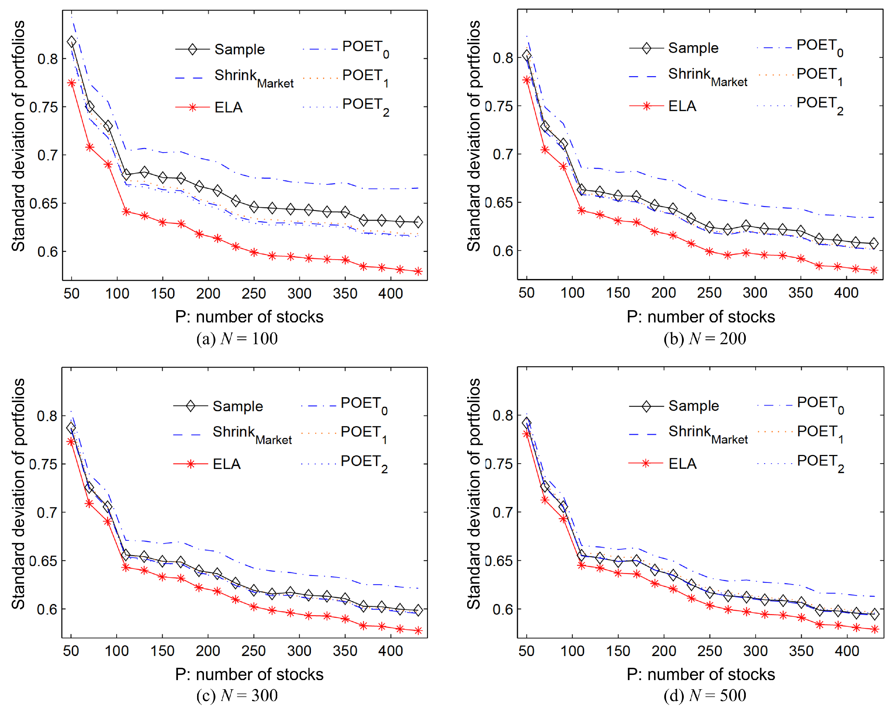
To understand how risk varies with the number of stocks, we alphabetically order the stocks by their symbols on the New York Stock Exchange and analyze growing subsets of stocks with $p=50$, $70,90,\dots ,430$. The risks associated with portfolios based on different methods are illustrated in Figure 5, with the ELA method highlighted by a red solid line. As the sample size N in the rolling window increases from 100 to 500 across the panels, the performance gap between the different estimation methods narrows, illustrating the homogeneity of the correlation matrix.

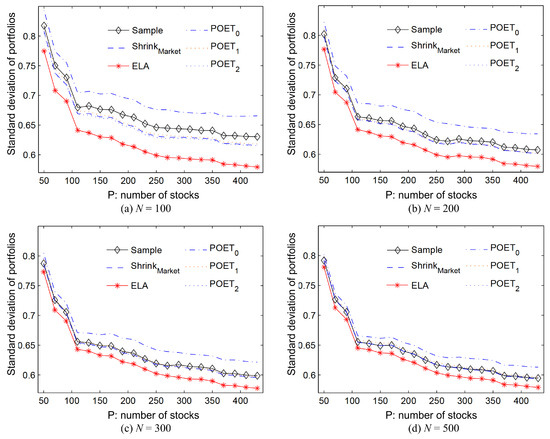
Figure 5. Portfolios of minimum risk based on different estimators of the covariance matrix.

Figure 5 shows that portfolios crafted using the ELA method consistently have the lowest risk compared to the POET_k methods, the shrinkage method, and the sample covariance matrix method, especially with smaller sample sizes of $N=100$ and $N=200$. Therefore, the ELA method is superior in constructing portfolios that minimize risk, is an effective tool for reducing portfolio risk, and is suitable for a wide range of sample sizes.

6. Conclusions

In this paper, we introduce a novel method called element-aggregation (ELA) estimation for the estimation of covariance matrices. The ELA method stands out due to its simplicity, low computational complexity, and applicability to both sparse and non-sparse matrices. Our theoretical analysis shows that the ELA method offers strong consistency while maintaining computational efficiency and dimensional independence, especially concerning block-wise covariance matrices.

In our numerical simulation study, we highlight the exceptional effectiveness of the ELA method in estimating correlation coefficient matrices and covariance matrices using diverse random samples. In comparison to established methods like POET and Rothman, the ELA method consistently either outperforms or equals them. The computational efficiency of our ELA method is complemented by a significant reduction in the relative estimation error for both correlation coefficients and covariance matrices.

In the real data analysis of the SP500 index stocks, the ELA method consistently generates portfolios with the lowest risk in comparison to other listed methods. This outcome is particularly pronounced in scenarios with smaller sample sizes, underscoring the potent ability of the ELA method to construct risk-minimized portfolios.

7. Future Work

This paper delves into the estimation of covariance matrices employing an elemental clustering approach, substantiating and evaluating the consistency and efficiency of the proposed methodology within the realm of high-dimensional data. The exponential growth in data volume and dimensionality due to advancements in computational and storage technologies has led to the emergence of ultra-high-dimensional and high-frequency datasets. Thus, the extensibility of the proposed method to these novel datasets, coupled with the demonstration of its consistency and efficacy, presents a significant avenue for future research. In addition, the exploration of computational strategies to increase efficiency under the constraints of ultra-high-dimensionality and to optimize the trade-off between computational resources and analytical accuracy is imperative. Furthermore, the proposed method has the potential to be integrated into diverse domains, such as psychology, social sciences, and genetic research. This also represents a promising direction for future research.

References

- Ledoit, O.; Wolf, M. The power of (non-) linear shrinking: A review and guide to covariance matrix estimation. J. Financ. Econ. 2022, 20, 187–218. [Google Scholar] [CrossRef]
- Zeileis, A. Econometric Computing with HC and HAC Covariance Matrix Estimators. J. Stat. Softw. 2004, 11, 1–17. [Google Scholar] [CrossRef]
- Ledoit, O.; Wolf, M. Nonlinear shrinkage of the covariance matrix for portfolio selection: Markowitz meets Goldilocks. Rev. Financ. Stud. 2017, 30, 4349–4388. [Google Scholar] [CrossRef]
- Schäfer, J.; Strimmer, K. A shrinkage approach to large-scale covariance matrix estimation and implications for functional genomics. Stat. Appl. Genet. Mol. 2005, 4, 1–32. [Google Scholar] [CrossRef]
- Tipping, M.E.; Bishop, C.M. Probabilistic principal component analysis. J. R. Stat. Soc. Ser. B Stat. Method. 1999, 61, 611–622. [Google Scholar] [CrossRef]
- Fan, J.; Fan, Y.; Lv, J. High dimensional covariance matrix estimation using a factor model. J. Econom. 2008, 147, 186–197. [Google Scholar] [CrossRef]
- Driscoll, J.C.; Kraay, A.C. Consistent covariance matrix estimation with spatially dependent panel data. Rev. Econ. Stat. 1998, 80, 549–560. [Google Scholar] [CrossRef]
- Pourahmadi, M. Maximum likelihood estimation of generalised linear models for multivariate normal covariance matrix. Biometrika 2000, 87, 425–435. [Google Scholar] [CrossRef]
- Ledoit, O.; Wolf, M. Improved estimation of the covariance matrix of stock returns with an application to portfolio selection. J. Empir. Financ. 2003, 10, 603–621. [Google Scholar] [CrossRef]
- Ledoit, O.; Wolf, M. A well-conditioned estimator for large-dimensional covariance matrices. J. Multivar. Anal. 2004, 88, 365–411. [Google Scholar] [CrossRef]
- Pepler, P.T.; Uys, D.W.; Nel, D.G. Regularized covariance matrix estimation under the common principal components model. Commun. Stat. Simul. Comput. 2018, 47, 631–643. [Google Scholar] [CrossRef]
- Bickel, P.J.; Levina, E. Regularized estimation of large covariance matrices. Ann. Stat. 2008, 36, 199–227. [Google Scholar] [CrossRef]
- El Karoui, N. Operator norm consistent estimation of large-dimensional sparse covariance matrices. Ann. Stat. 2008, 36, 2717–2756. [Google Scholar] [CrossRef]
- Rothman, A.J.; Levina, E.; Zhu, J. Generalized thresholding of large covariance matrices. J. Am. Stat. Assoc. 2009, 104, 177–186. [Google Scholar] [CrossRef]
- Cai, T.; Liu, W. Adaptive thresholding for sparse covariance matrix estimation. J. Am. Stat. Assoc. 2011, 106, 672–684. [Google Scholar] [CrossRef]
- Cai, T.T.; Yuan, M. Adaptive covariance matrix estimation through block thresholding. Ann. Stat. 2012, 40, 2014–2042. [Google Scholar] [CrossRef]
- Lam, C.; Fan, J. Sparsistency and rates of convergence in large covariance matrix estimation. Ann. Stat. 2009, 37, 4254–4278. [Google Scholar] [CrossRef] [PubMed]
- Rothman, A.J. Positive definite estimators of large covariance matrices. Biometrika 2012, 99, 733–740. [Google Scholar] [CrossRef]
- Fan, J.; Liao, Y.; Mincheva, M. Large covariance estimation by thresholding principal orthogonal complements. J. R. Stat. Soc. Ser. B Stat. Method. 2013, 75, 603–680. [Google Scholar] [CrossRef]
- Onnela, J.P.; Chakraborti, A.; Kaski, K.; Kertesz, J.; Kanto, A. Dynamics of market correlations: Taxonomy and portfolio analysis. Phys. Rev. E 2003, 68, 056110. [Google Scholar] [CrossRef]
- Matteson, D.; Tsay, R.S. Multivariate Volatility Modeling: Brief Review and a New Approach; Manuscript, Booth School of Business, University of Chicago: Chicago, IL, USA, 2011. [Google Scholar]
- Qian, J. Shrinkage Estimation of Nonlinear Models and Covariance Matrix. Doctoral Thesis, National University of Singapore, Department of Statistics and Applied Probability, Singapore, 2012. Available online: https://core.ac.uk/download/pdf/48656486.pdf (accessed on 27 March 2024).
- Jiang, H.; Saart, P.W.; Xia, Y. Asymmetric conditional correlations in stock returns. Ann. Appl. Stat. 2016, 10, 989–1018. [Google Scholar] [CrossRef]
- Elton, E.J.; Gruber, M.J. Estimating the dependence structure of share prices–implications for portfolio selection. J. Financ. 1973, 28, 1203–1232. [Google Scholar]
- Liu, S. Matrix results on the Khatri-Rao and Tracy-Singh products. Linear Algebra Appl. 1999, 289, 267–277. [Google Scholar] [CrossRef]
- Bollerslev, T. Modeling the coherence in short-run nominal exchange rates: A multivariate generalized ARCH model. Rev. Econ. Stat. 1990, 72, 498–505. [Google Scholar] [CrossRef]
- Hansen, P.R.; Lunde, A. A forecast comparison of volatility models: Does anything beat a GARCH(1,1)? J. Appl. Econ. 2005, 20, 873–889. [Google Scholar] [CrossRef]
- Aghamohammadi, A.; Dadashi, H.; Sojoudi, M.; Sojoudi, M.; Tavoosi, M. Optimal portfolio selection using quantile and composite quantile regression models. Commun. Stat. Simul. Comput. 2022, 1–11. [Google Scholar] [CrossRef]
- Zhang, Z.; Yue, M.; Huang, L.; Wang, Q.; Yang, B. Large portfolio allocation based on high-dimensional regression and Kendall’s Tau. Commun. Stat. Simul. Comput. 2023, 1–13. [Google Scholar] [CrossRef]
- Golub, G.H.; Van Loan, C.F. Matrix Computations; Johns Hopkins University Press: Baltimore, MD, USA, 2013. [Google Scholar]
Disclaimer/Publisher’s Note: The statements, opinions and data contained in all publications are solely those of the individual author(s) and contributor(s) and not of MDPI and/or the editor(s). MDPI and/or the editor(s) disclaim responsibility for any injury to people or property resulting from any ideas, methods, instructions or products referred to in the content. |
© 2024 by the author. Licensee MDPI, Basel, Switzerland. This article is an open access article distributed under the terms and conditions of the Creative Commons Attribution (CC BY) license (https://creativecommons.org/licenses/by/4.0/).