Shrinkage Testimator for the Common Mean of Several Univariate Normal Populations

Abstract

The challenge of combining two unbiased estimators is a common occurrence in applied statistics, with significant implications across diverse fields such as manufacturing quality control, medical research, and the social sciences. Despite the widespread relevance of estimating the common population mean $\mu$, this task is not without its challenges. A particularly intricate issue arises when the variations within populations are unknown or possibly unequal. Conventional approaches, like the two-sample t-test, fall short in addressing this problem as they assume equal variances among the two populations. When there exists prior information regarding population variances $({\sigma }_i^2,i=1,2)$, with the consideration that ${\sigma }_1^2$ and ${\sigma }_2^2$ might be equal, a hypothesis test can be conducted: $H_0:{\sigma }_1^2={\sigma }_2^2$ versus $H_1:{\sigma }_1^2\ne {\sigma }_2^2$. The initial sample is utilized to test $H_0$, and if we fail to reject $H_0$, we gain confidence in incorporating our prior knowledge (after testing) to estimate the common mean $\mu$. However, if $H_0$ is rejected, indicating unequal population variances, the prior knowledge is discarded. In such cases, a second sample is obtained to compensate for the loss of prior knowledge. The estimation of the common mean $\mu$ is then carried out using either the Graybill–Deal estimator (GDE) or the maximum likelihood estimator (MLE). A noteworthy discovery is that the proposed preliminary testimators, denoted as ${\widehat{\mu }}_{P{T}_1}$ and ${\widehat{\mu }}_{P{T}_2}$, exhibit superior performance compared to the widely used unbiased estimators (GDE and MLE).

1. Introduction

The problem of combining two unbiased estimators arises frequently in applied statistics, where it has important implications in a wide range of fields, from quality control in manufacturing to medical research and social sciences [1,2,3]. For instance, in the context of manufacturing, it is essential to ensure that the means of different production lines are within specified quality standards. By using the common mean inference, you can determine whether the means of these production lines are within specified quality standards. If one line’s mean falls outside the acceptable range, it could signal a quality issue. In clinical trials, researchers often need to compare the effectiveness of different treatments or drugs. The common mean approach can help determine whether a particular treatment yields statistically different results in terms of patient outcomes, such as recovery times or symptom alleviation.

The technique of combining and analyzing data from several independent studies on a specific topic or research question is referred to as meta-analysis [3]. The goal of meta-analysis is to obtain a more accurate and reliable estimate of the overall effect size or treatment effect than what can be achieved by any individual study alone [3,4]. It provides a systematic and quantitative approach to synthesizing evidence from various studies, allowing researchers to draw more robust conclusions and make generalizations [3].

A well-known context of this problem occurred when Meier [2] was asked to draw inferences about the mean of albumin in plasma protein in human subjects based on results from four experiments [2], shown in

Table 1. Albumin in plasma protein of four different experiments.

Experiment	${\mathit{n}}_{\mathit{i}}$	Mean	Variance
A	12	62.30	12.99
B	15	60.30	7.84
C	7	59.50	33.43
D	16	61.50	18.51

.

Another scenario happened when Eberhardt et al. [5] had results from four experiments about nonfat milk powder and the problem was to draw inferences about the mean Selenium in nonfat milk powder by combining the results from four methods (

Table 2. Selenium content in nonfat milk powder using four methods.

Methods	${\mathit{n}}_{\mathit{i}}$	Mean	Variance
Atomic absorption spectrometry	8	105.00	85.71
Neutron activation:
(1) Instrumental	12	109.75	20.75
(2) Radiochemical	14	109.50	2.73
Isotope dilution mass spectrometry	8	113.25	33.64

).

Despite the broad applicability of the common mean, $\mu$, estimating it is not without difficulties. One of the most difficult problems emerges when the population variations are unknown or maybe unequal. Traditional approaches for addressing this issue, such as the two-sample t-test, are insufficient since they assume equal variances and are not designed for combining and analyzing data from several independent studies on a specific topic or research question.

To formulate the present problem, we assume only that there are two normal populations with a common mean, but with unknown and possibly unequal variances ${\sigma }_1^2,\dots ,{\sigma }_k^2>0$. Let us assume that we have independent and identically distributed ($i.i.d$) observations $X_{i1},\dots ,X_{i{n}_i}$ from $N(\mu ,{\sigma }_i^2)$, $i=1,2$ and define ${\overline{X}}_i$ and $S_i$ are given as

$$\begin{array}{cc}\hfill {\overline{X}}_i& =\sum _{j=1}^{n_i}\frac{X_{ij}}{n_i},S_i=\sum _{j=1}^{n_i}{(X_{ij}-{\overline{X}}_i)}^2,\hfill \end{array}$$

(1)

where ${\overline{X}}_i\sim N(\mu ,{\sigma }_i^2/n_i)$, $S_i\sim {\sigma }_i{\chi }_{n_i-1}^2$. Note that these statistics, $\{{\overline{X}}_i,S_i,i=1,2\}$, are all mutually independent. Again, it can be noted that $\{{\overline{X}}_1,S_1,{\overline{X}}_2,S_2\}$ are minimal sufficient statistics for $(\mu ,{\sigma }_1^2,{\sigma }_2^2)$ but are not complete. As a result, one cannot obtain the uniformly minimum-variance unbiased estimator (UMVUE) if it exists using the standard Rao–Blackwell theorem on an unbiased estimator for estimating the common mean $\mu$.

The natural meta-analysis question now is the problem of combining several estimates of an unknown quantity to obtain an estimate of improved precision. A similar problem arises in the analysis of incomplete block experiments. The “intra-block” and “inter-block” estimates of varietal means have different variances, and the recovery of “inter-block information” is an attempt to combine these estimates in the most efficient manner. In the case when the two population variances are completely known, the common mean $\mu$ can easily be estimated as

$$\begin{array}{cc}\hfill \widehat{\mu }& =\left(\sum _{i=1}^2\frac{n_i}{{\sigma }_i^2}{\overline{X}}_i\right)/\left(\sum _{i=1}^2\frac{n_i}{{\sigma }_i^2}\right),\hfill \end{array}$$

(2)

which is the UMVUE, the best linear unbiased estimator (BLUE), and the maximum likelihood estimator (MLE) with a variance given as

$$\begin{array}{c}\hfill \mathrm{Var}\left(\widehat{\mu }\right)=\frac{1}{{\sum }_1^2\left(n_i/{\sigma }_i^2\right)}.\end{array}$$

(3)

In our present problem, the population variances are unknown and possibly unequal. The most appealing unbiased estimator of $\widehat{\mu }$ is the Graybill–Deal estimate (GDE) [6], given as

$$\begin{array}{cc}\hfill {\widehat{\mu }}_{GD}& =\left(\sum _{i=1}^2\frac{n_i}{s_i^2}{\overline{X}}_i\right)/\left(\sum _{i=1}^2\frac{n_i}{s_i^2}\right),\hfill \end{array}$$

(4)

with

$$\begin{array}{c}\hfill \mathrm{Var}\left({\widehat{\mu }}_{GD}\right)=E\left[\left(\sum _{i=1}^2\left(\frac{n_i{\sigma }_i^2}{s_i^4}\right)\right)/{\left(\sum _{i=1}^2\left(\frac{n_i}{s_i^2}\right)\right)}^2\right],\end{array}$$

(5)

where $s_i^2=S_i/(n_i-1),i=1,2.$ For the two-sample case, the GDE [6] showed first that an unbiased estimator has a smaller variance than either sample mean provided that both sample sizes are greater than 10. Since then, several papers have been written generalizing and extending their findings [7,8,9,10,11] and the references therein. On the other hand, Meier [2] suggested a method for setting an approximate confidence interval for $\mu$ centered at ${\widehat{\mu }}_{GD}$. Furthermore, [12,13] developed approximate confidence intervals centered at ${\widehat{\mu }}_{GD}$. The properties of such estimators have received a lot of attention in the literature. We would like to highlight the contributions of Kifle et al. [1], Sinha et al. [3], Sinha [14], Hartung [15], and Krishnamoorthy and Moore [16] in particular.

Even though many generalizations of ${\widehat{\mu }}_{GD}$ have been proposed in recent years, it still commonly remains one of the central figures in statistical modeling and methods in meta-analysis due to its natural appeal. We may have prior information that the variances ${\sigma }_1^2$ and ${\sigma }_2^2$ may be equal. Then, we can test the hypothesis $H_0:{\sigma }_1^2={\sigma }_2^2$ versus $H_1:{\sigma }_1^2\ne {\sigma }_2^2$ and then estimate the common mean $\widehat{\mu }$ of these two independent normal populations depending on the outcome of this test. Stein [17] introduced and thoroughly discussed the preliminary test shrinkage estimator. His work had a profound impact on the field of statistical estimation, particularly for the common mean problem with unknown variances. His approach has inspired various developments and applications in statistics and has become a foundation for the use of shrinkage estimators in modern statistical practice. Thompson [18] proposed a shrinkage technique, given as

$$\omega =q{\theta }_0+(1-q)\theta ,$$

(6)

for improving the existing estimator of parameter $\theta$ and estimating the mean, which lowers the mean square error (MSE) of the UMVUE of the mean of a population, is considered. It was noted that the shrinkage estimator outperforms the usual estimator if the guess value of q is chosen in a way that aligns with reality. Therefore, rather than considering q as a fixed constant in the shrinkage estimator, one should consider it as a weight that falls between 0 and 1. In this case, q can be treated as a continuous function of some relevant statistics, with the expectation that its value will drop monotonically as $(\theta -{\theta }_0)$ increases. Other researchers, like, Walker, Schuurmann, and Raghunathan [19], also proposed a testimator for the mean of a normal distribution. It was further noted in the literature that when prior information is available, the shrinkage estimators for the parameters of various distributions perform better than the usual estimators in terms of the mean square error when the estimated value is close to the true value [18,20,21].

If we assume that the prior knowledge about population variances $({\sigma }_i^2,i=1,2)$ is available and that the variances ${\sigma }_1^2$ and ${\sigma }_2^2$ may be equal, we can test the hypothesis $H_0:{\sigma }_1^2={\sigma }_2^2$ versus $H_1:{\sigma }_1^2\ne {\sigma }_2^2$. The first stage sample is used to test $H_0$ and if we fail to reject $H_0$, we feel comfortable in using prior knowledge (having tested it) to estimate the common mean $\mu$. However, if $H_0$ is rejected, we discard our prior knowledge and obtain a second sample to make up for the loss of the prior knowledge and estimate the common mean $\mu$ using GDE or MLE. This type of adaptive estimator based on a preliminary test has been used by many researchers [22,23].

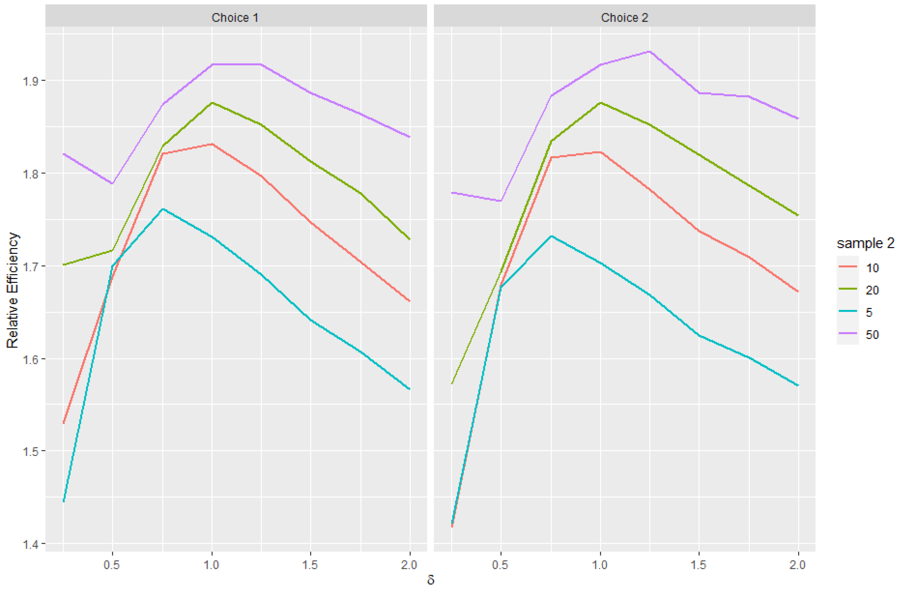
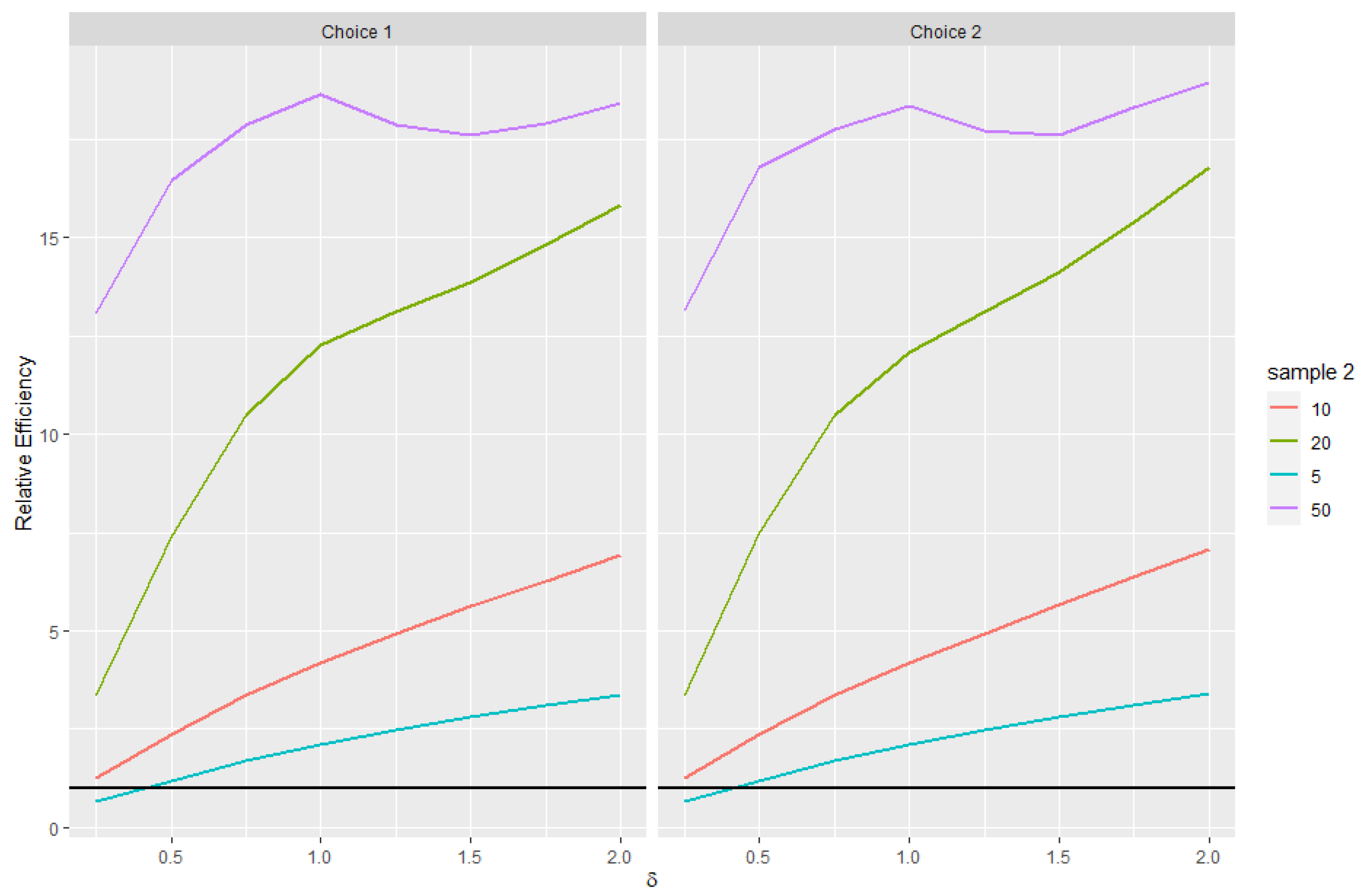
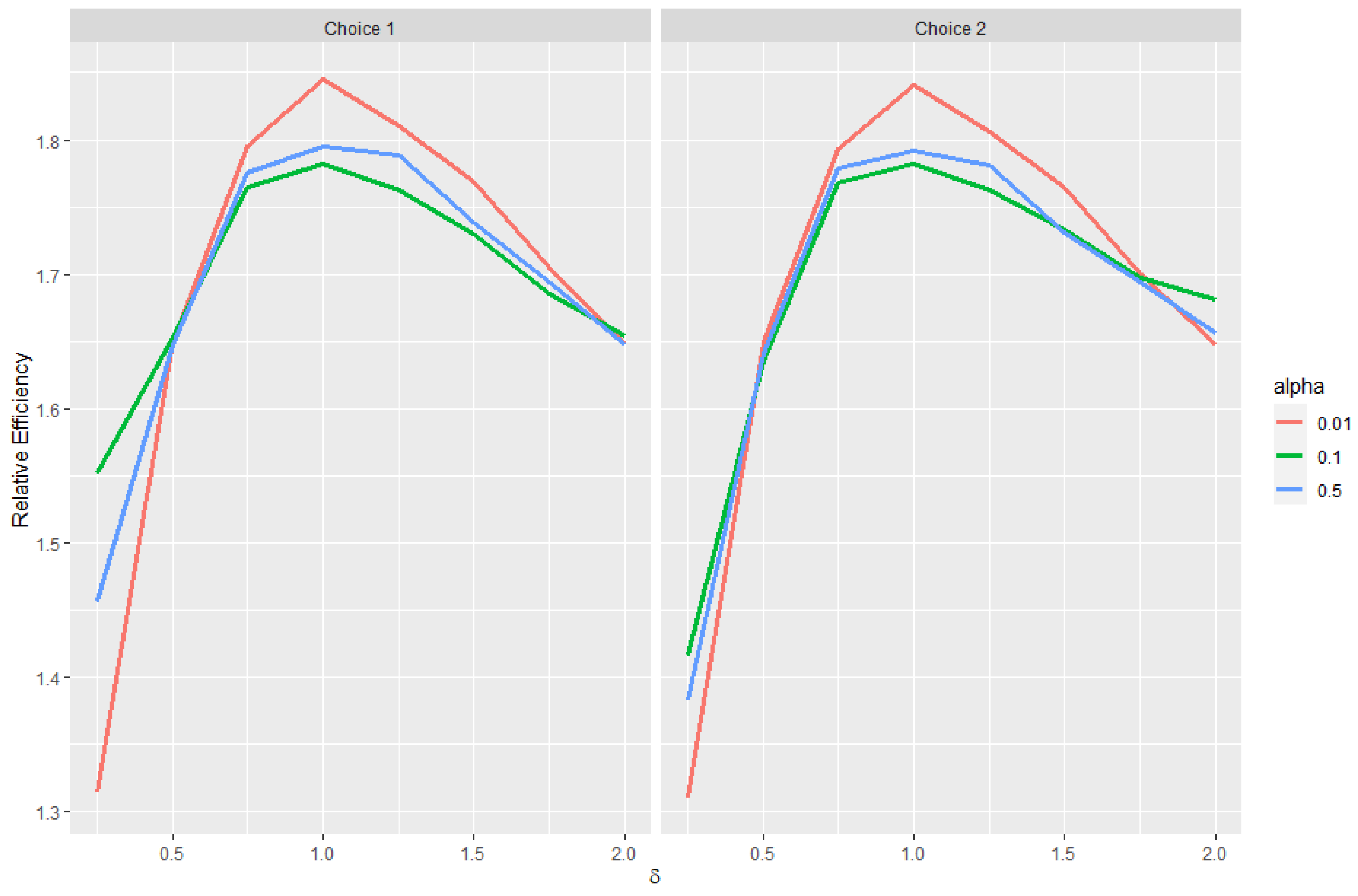
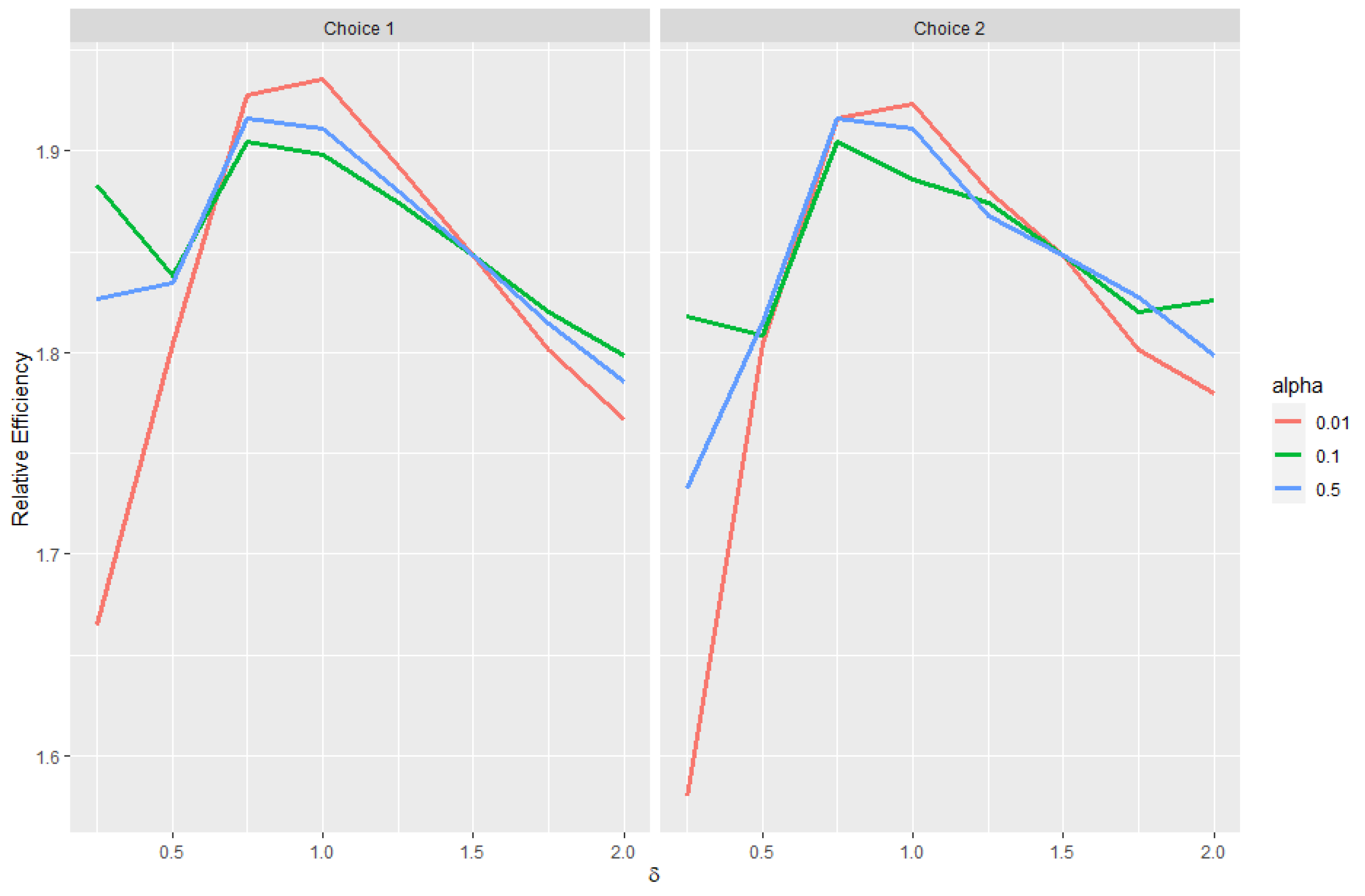
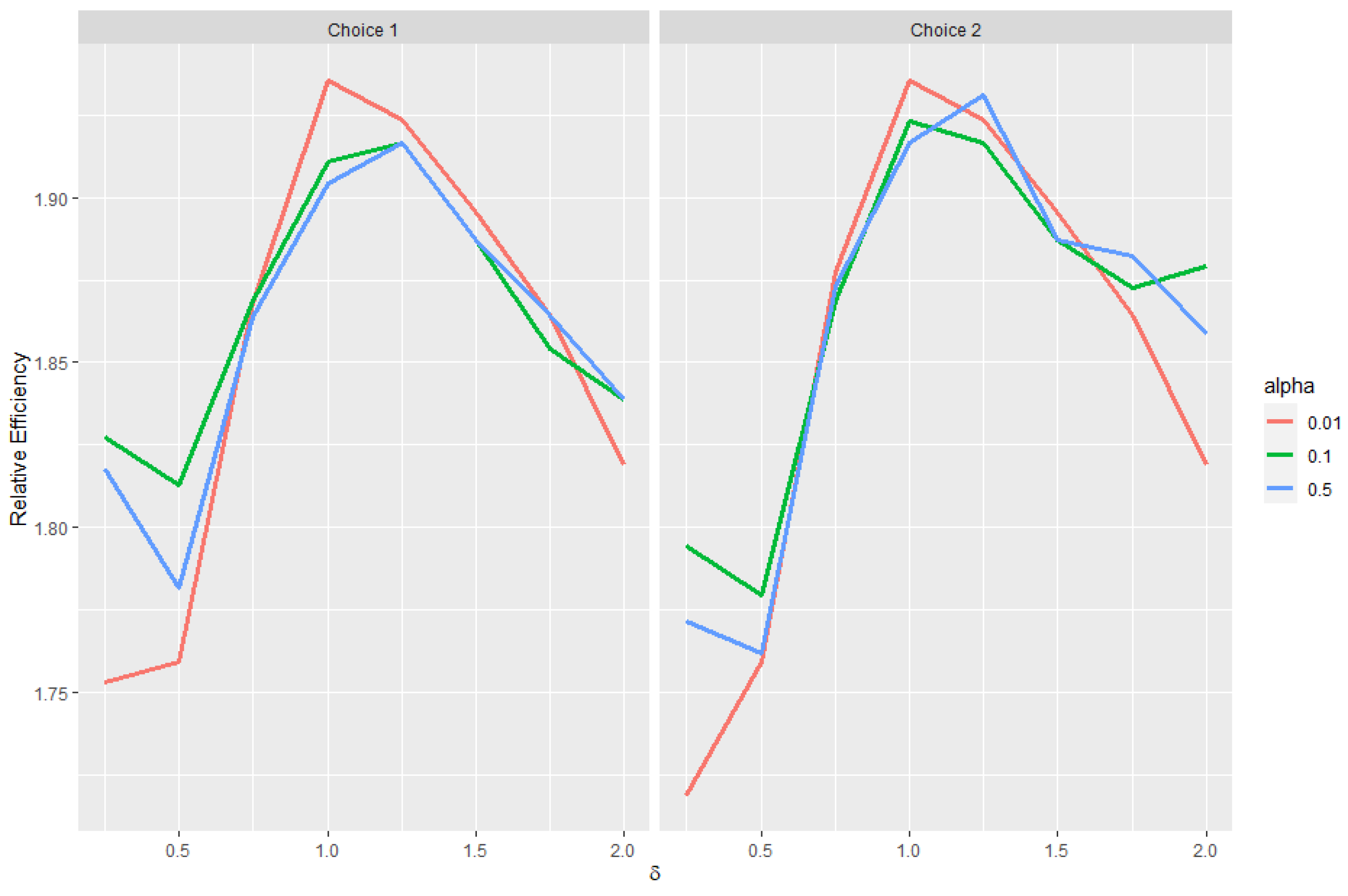
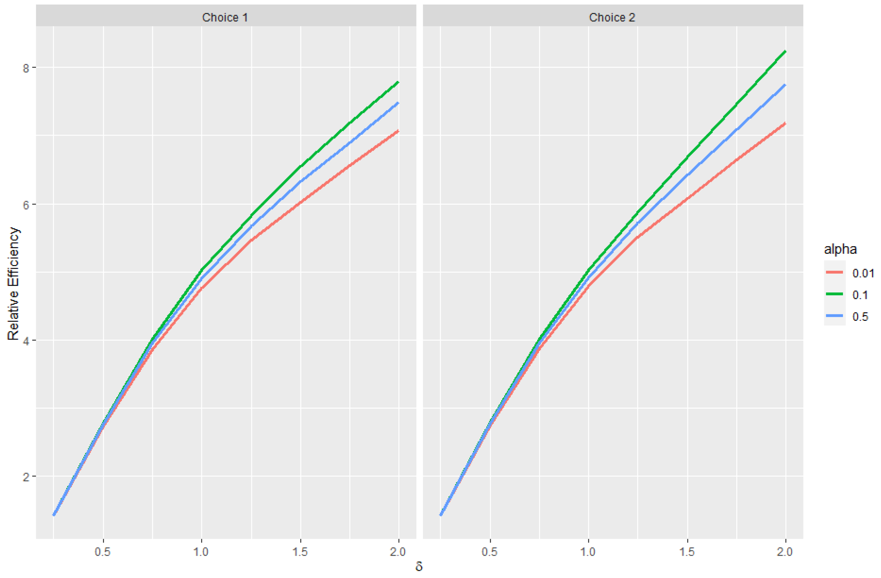
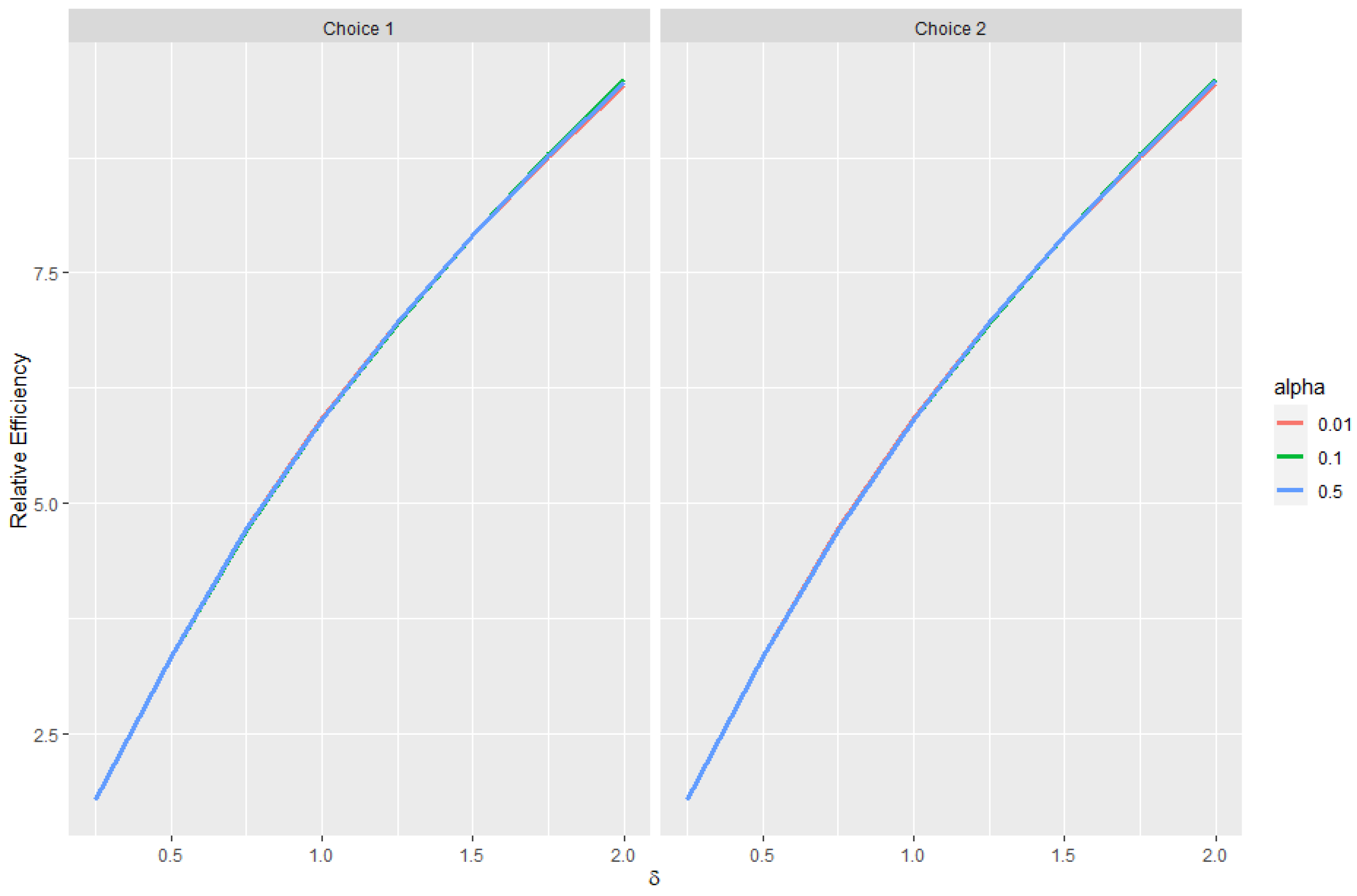
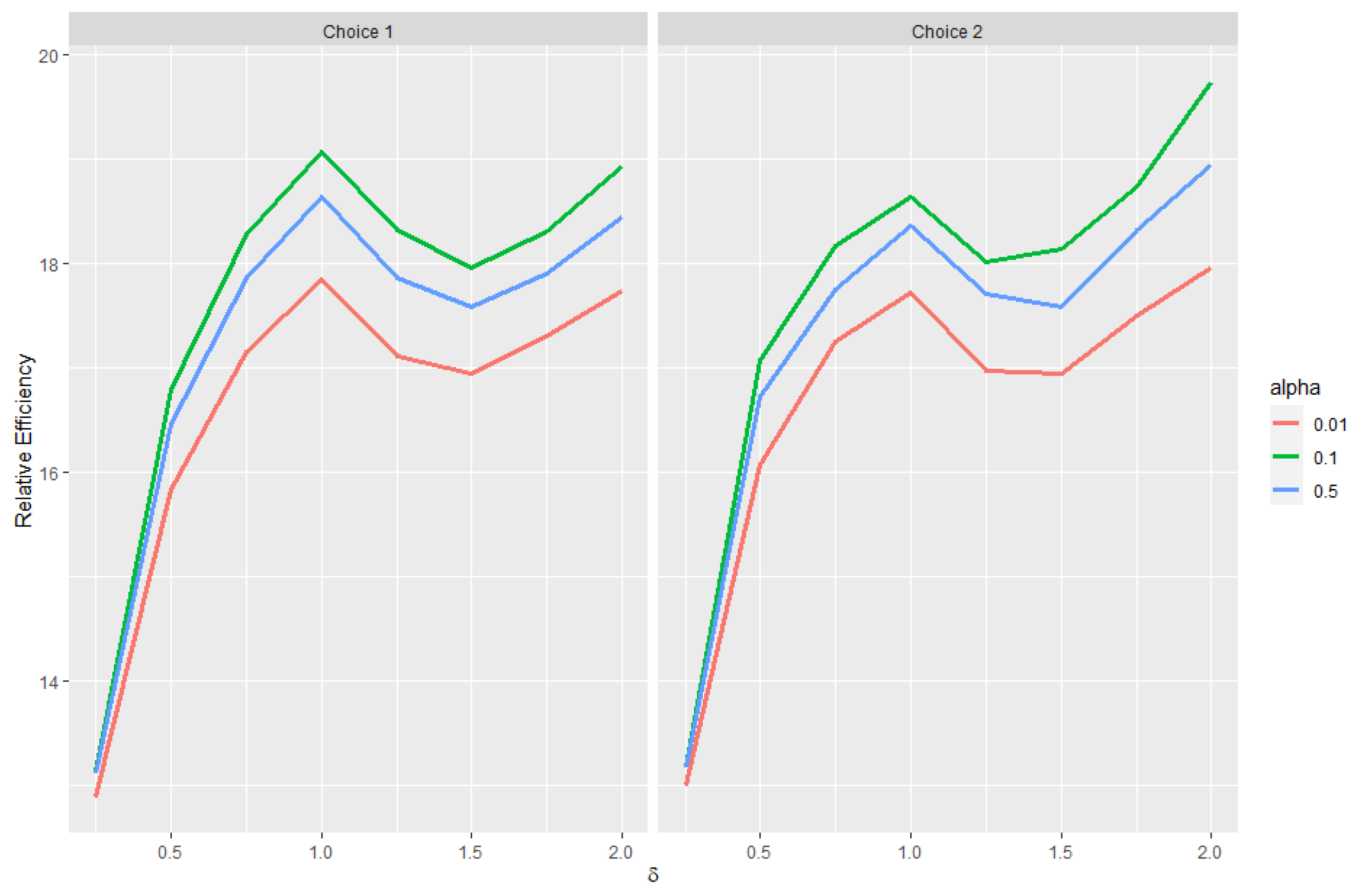
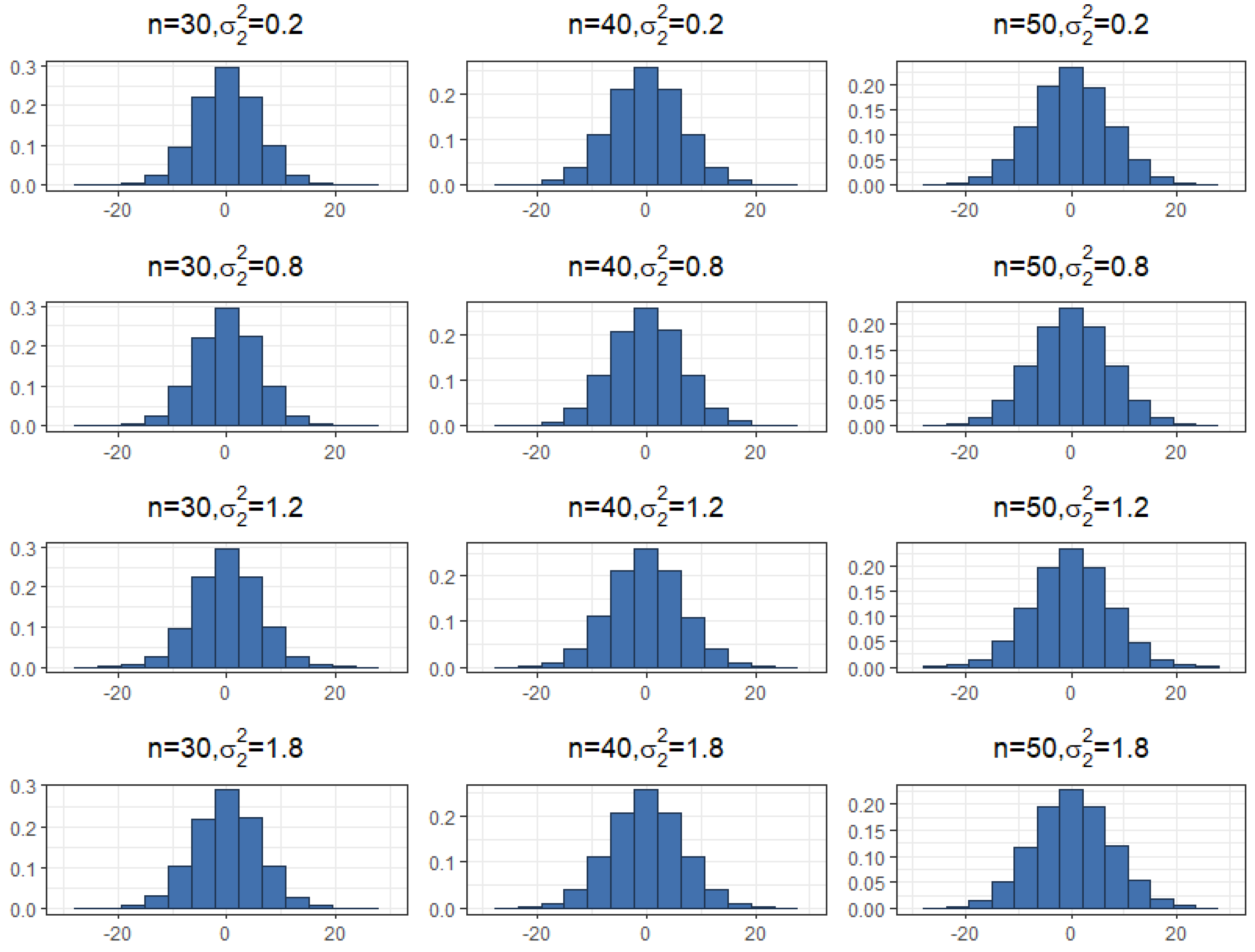
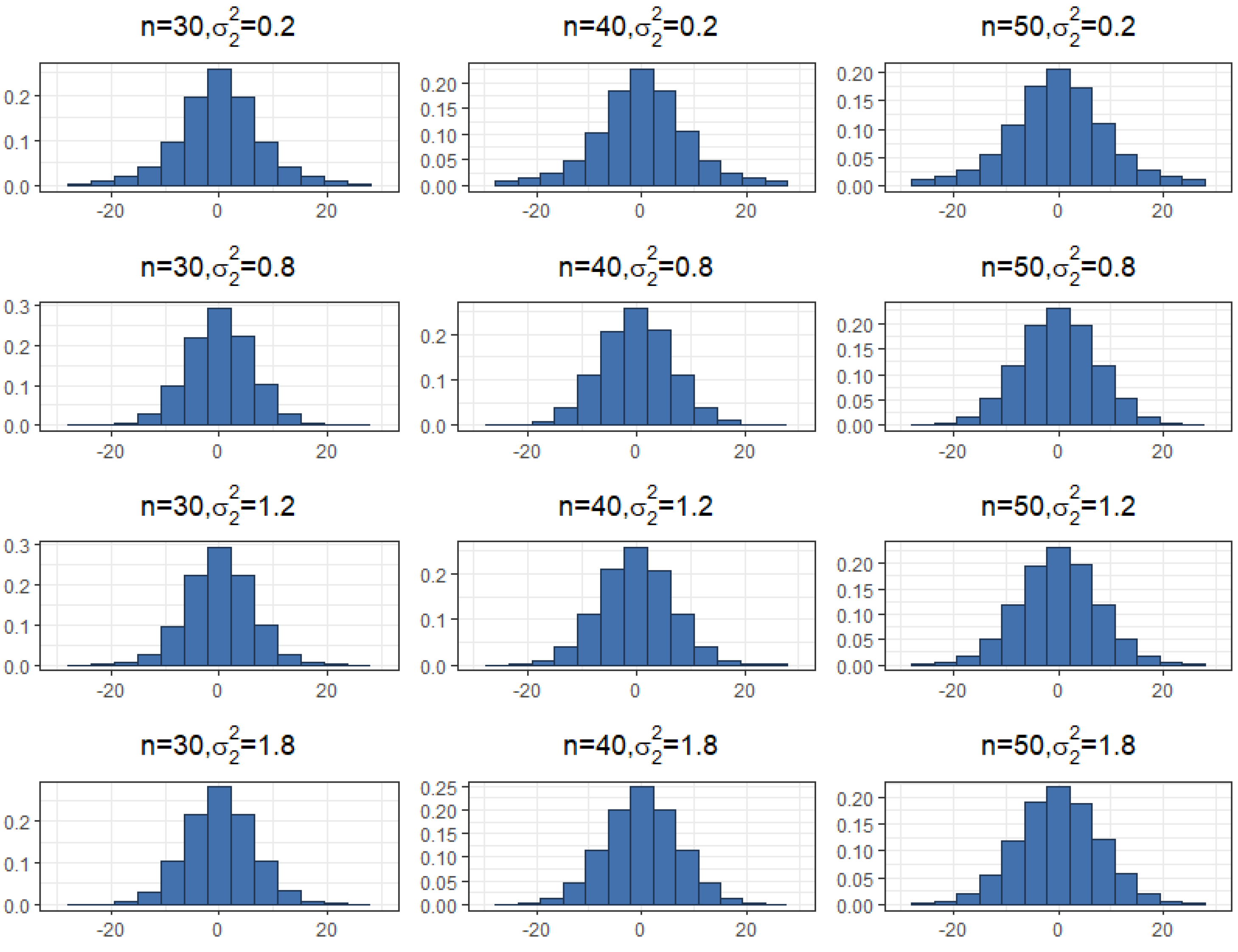
Estimating and evaluating hypotheses about the common means of different univariate normal populations is an important problem. This study attempts to propose a preliminary testimator for the common mean $\mu$ with unknown and unequal variances. The preliminary testimator thus produced will be studied for its behavior when the expressions of its bias, MSE, and Relative Efficiency (RE) are determined and their performance will be evaluated. The proposed method incorporates preliminary testing to assess the equality of population variances before estimating the common mean $\mu$. When significant differences in variances are detected, the preliminary test shrinkage estimator adjusts the weight assigned to each sample mean, shrinking estimates from populations with smaller sample variances towards the overall mean. This is the main motivation behind this revisit to the common mean $\mu$ problem and filling certain gaps analytically as well as computationally while proposing a preliminary test shrinkage estimator.

2. Materials and Methods

It is natural to test a null hypothesis with the prior, uncertain non-sample information in hand. This is followed by the testimator. A testimator is a two-step estimator that estimates an important parameter based on the results of a preliminary test. For estimating the common mean $\mu$, we consider the hypothesis

$$H_0:{\sigma }_1^2={\sigma }_2^{2}vs.H_1:{\sigma }_1^2\ne {\sigma }_2^2.$$

(7)

We define our proposed preliminary testimator for the common mean $\mu$ as

$${\widehat{\mu }}_{PT}=\left\{\begin{array}{cc}{\mu }_{Grand}=\frac{n_1\overline{X}+n_2\overline{Y}}{n_1+n_2}\hfill & ,\mathrm{if}{c}_{1\alpha }<F<c_{2\alpha }\hfill \\ {\widehat{\mu }}_{UE}\hfill & ,\mathrm{if}F<c_{1\alpha }\mathrm{or}F>c_{2\alpha },\hfill \end{array}\right.$$

(8)

where ${\widehat{\mu }}_{UE}$ is the unbiased estimator of $\mu$. We may rewrite the above equation as

$${\widehat{\mu }}_{PT}={\mu }_{Grand}\left\{\mathbf{I}\left(c_{1\alpha }<F<c_{2\alpha }\right)\right\}+{\widehat{\mu }}_{UE}\left\{\mathbf{I}\left(F<c_{1\alpha }\mathrm{or}F>c_{2\alpha }\right)\right\},$$

(9)

where $\mathbf{I}(·)$ is the indicator function, defined as $\mathbf{I}\left(A\right)=1$ if A is true and $\mathbf{I}\left(A\right)=0$ if A is false, and $F=s_1^2/s_2^2$ is the F-test statistic. The more this ratio deviates from 1, the stronger the evidence is for unequal population variances. To find the F critical values $(c_{1\alpha }$ and $c_{2\alpha })$, we look at two choices:

• Choice 1: Equal tail probability by fixing $c_{1\alpha }$ and $c_{2\alpha }$ to $\frac{\alpha }{2}$. The hypothesis that the two variances are equal is rejected if $F>F_{\frac{\alpha }{2},{\nu }_1,{\nu }_2}\mathrm{or}F<F_{1-\frac{\alpha }{2},{\nu }_1,{\nu }_2}$, where ${\nu }_i=n_i-1,i=1,2$.
• Choice 2: Under the alternative hypothesis, $F=\frac{s_1^2/{\sigma }_1^2}{s_2^2/{\sigma }_2^2}=\frac{F}{\theta }\sim F_{{\nu }_1,{\nu }_2}$. Then, $1-\alpha =P_r(c_{1\alpha }<F/\theta <c_{2\alpha })$, where $\theta ={\sigma }_1^2/{\sigma }_2^2$. It is not unique in choosing $c_{1\alpha }$ and $c_{2\alpha }$ for the given $(1-\alpha )$. In order to make it unique, we minimize the length between the upper and lower bounds as $L=F(\frac{1}{c_{1\alpha }}-\frac{1}{C_{2\alpha }})$. The expected length, L, is then given as $E\left(F\right)(\frac{1}{c_{1\alpha }}-\frac{1}{C_{2\alpha }})$. So, the critical values may be found by minimizing $(\frac{1}{c_{1\alpha }}-\frac{1}{C_{2\alpha }})$ subject to $1-\alpha =P_r(c_{1\alpha }<F<c_{2\alpha })$.

2.1. The GDE of the Common Mean

The famous and most widely used estimator is the GDE [6] estimator, which is an unbiased estimator of the common mean $\mu$ which is uniformly better than either $X_i,i=1,2$ in that $n_i,i=1,2$ are both larger than ten. We define our proposed testimator for the common mean as

$${\widehat{\mu }}_{P{T}_1}=\left\{\begin{array}{cc}{\mu }_{Grand}=\frac{n_1{\overline{X}}_1+n_2{\overline{X}}_2}{n_1+n_2}\hfill & ,\mathrm{if}{c}_{1\alpha }<F<c_{2\alpha }\hfill \\ {\widehat{\mu }}_{GD}=\left(\sum _{i=1}^2\frac{n_i}{s_i^2}{\overline{X}}_i\right)/\left(\sum _{i=1}^2\frac{n_i}{s_i^2}\right)\hfill & ,\mathrm{if}F<c_{1\alpha }\mathrm{or}F>c_{2\alpha }.\hfill \end{array}\right.$$

(10)

The ${\widehat{\mu }}_{GD}$ in the equation above, can be expressed as ${\widehat{\mu }}_{GD}={\overline{X}}_1ϵ+{\overline{X}}_2\left(1-ϵ\right)$, where $ϵ=n_1{s}_2^2/\left(n_2{s}_1^2+n_1{s}_2^2\right)$. Notice that $ϵ$ is the function of $s_1^2,s_2^2$. Then, we may also rewrite ${\mu }_{Grand}$ in the above equation as ${\mu }_{Grand}={\overline{X}}_{1}B+{\overline{X}}_2\left(1-B\right)$, where $B=n_1/\left(n_1+n_2\right)$. Notice that B is the function of $n_1,n_2$. Then, we revise our proposed testimator ${\widehat{\mu }}_{P{T}_1}$ as

$$\begin{array}{cc}\hfill {\widehat{\mu }}_{P{T}_1}& ={\mu }_{Grand}\mathbf{I}(c_{1\alpha }<F<c_{2\alpha })+{\widehat{\mu }}_{GD}\mathbf{I}(F<c_{1\alpha }|F>c_{2\alpha })\hfill \\ \hfill & =\left\{{\overline{X}}_{1}B+{\overline{X}}_2\left(1-B\right)\right\}\mathbf{I}\left(A\right)+\left\{{\overline{X}}_1ϵ+{\overline{X}}_2\left(1-ϵ\right)\right\}\mathbf{I}\left(A^c\right)\hfill \\ \hfill & ={\overline{X}}_1\left\{ϵ\mathbf{I}\left(A^c\right)+B\mathbf{I}\left(A\right)\right\}+{\overline{X}}_2\left\{\left(1-ϵ\right)\mathbf{I}\left(A^c\right)+\left(1-B\right)\mathbf{I}\left(A\right)\right\},\hfill \end{array}$$

(11)

where $\mathbf{I}(·)$ is the indicator function, defined as $\mathbf{I}\left(A\right)=1$ if A is true and $\mathbf{I}\left(A\right)=0$ if A is false.

2.1.1. Bias of Preliminary Testimator ${\widehat{\mu }}_{P{T}_1}$

The bias of the proposed preliminary testimator is equal to $E\left({\widehat{\mu }}_{P{T}_1}\right)-\mu$, where

$$\begin{array}{cc}\hfill E\left({\widehat{\mu }}_{P{T}_1}\right)& =E\left[E\left({\overline{X}}_1\left\{ϵ\mathbf{I}\left(A^c\right)+B\mathbf{I}\left(A\right)\right\}+{\overline{X}}_2\left\{\left(1-ϵ\right)\mathbf{I}\left(A^c\right)+\left(1-B\right)\mathbf{I}\left(A\right)\right\}|s_1^2,s_2^2\right)\right]\hfill \\ \hfill & =E\left[E\left(\left\{{\overline{X}}_{1}B+{\overline{X}}_2\left(1-B\right)\right\}\mathbf{I}\left(A\right)+\left\{{\overline{X}}_1ϵ+{\overline{X}}_2\left(1-ϵ\right)\right\}\mathbf{I}\left(A^c\right)|s_1^2,s_2^2\right)\right]\hfill \\ \hfill & =E_{s_1^2,s_2^2}\left[\mu \mathbf{I}\left(A\right)+\mu \mathbf{I}\left(A^c\right)\right]\hfill \\ \hfill & =\mu .\hfill \end{array}$$

(12)

Our proposed preliminary testimator ${\widehat{\mu }}_{P{T}_1}$ is an unbiased estimator for a common mean $\mu$.

2.1.2. Mean Square Error of Preliminary Testimator ${\widehat{\mu }}_{P{T}_1}$

The MSE of ${\widehat{\mu }}_{P{T}_1}$ can be expressed as

$$\begin{array}{cc}\hfill \mathrm{MSE}\left({\widehat{\mu }}_{P{T}_1}\right)& =E{({\widehat{\mu }}_{P{T}_1}-\mu )}^2\hfill \\ \hfill & =E{\left\{\left({\overline{X}}_1\psi +{\overline{X}}_2\Psi \right)-\mu \right\}}^2\hfill \\ \hfill & =E\left({\overline{X}}_1^2{\psi }^2+{\overline{X}}_2^2{\Psi }^2-2{\overline{X}}_1\psi \mu -2{\overline{X}}_2\Psi \mu +2{\overline{X}}_1\psi {\overline{X}}_2\Psi +{\mu }^2\right)\hfill \\ \hfill & =E\left\{E\left[\left({\overline{X}}_1^2{\psi }^2+{\overline{X}}_2^2{\Psi }^2-2{\overline{X}}_1\psi \mu -2{\overline{X}}_2\Psi \mu +2{\overline{X}}_1\psi {\overline{X}}_2\Psi +{\mu }^2\right)|s_1^2,s_2^2\right]\right\}\hfill \\ \hfill & =\frac{{\sigma }_1^2}{n_1}{E}_{s_1^2,s_2^2}\left({\psi }^2\right)+\frac{{\sigma }_2^2}{n_2}{E}_{s_1^2,s_2^2}\left({\Psi }^2\right)+{\mu }^2{E}_{s_1^2,s_2^2}\left\{(\psi +\Psi )\left[(\psi +\Psi )-2\right]+1\right\},\hfill \end{array}$$

where $\psi =ϵ\mathbf{I}\left(A^c\right)+B\mathbf{I}\left(A\right)$ and $\Psi =\left(1-ϵ\right)\mathbf{I}\left(A^c\right)+\left(1-B\right)\mathbf{I}\left(A\right)$. Without loss of generality, $\mu =0$. Therefore, our above equation for $\mathrm{MSE}\left({\widehat{\mu }}_{P{T}_1}\right)$ can be defined as

$$\mathrm{MSE}\left({\widehat{\mu }}_{P{T}_1}\right)=\frac{{\sigma }_1^2}{n_1}{E}_{s_1^2,s_2^2}\left({\psi }^2\right)+\frac{{\sigma }_2^2}{n_2}{E}_{s_1^2,s_2^2}\left({\Psi }^2\right)$$

(13)

2.2. The MLE of the Common Mean

Pal et al. [24] revisited the common mean problem by elucidating the structure of the MLE, and comparing it with the GDE. It was found that the MLE has better overall performance than the popular GDE. It can be noted that the MLE for the common mean $\mu$ does not have a closed expression when ${\sigma }_i^2$ is unknown and, as a result, the exact sampling distribution is impossible to derive [24].

The MLEs of ${\widehat{\mu }}_{\mathrm{ML}},{\widehat{\sigma }}_{1\left(\mathrm{ML}\right)}^2$, and ${\widehat{\sigma }}_{2\left(\mathrm{ML}\right)}^2$ are defined as

$$\begin{array}{cc}\hfill {\widehat{\sigma }}_{1\left(\mathrm{ML}\right)}^2& =\left(S_1/n_1\right)+{\left\{n_2{\widehat{\sigma }}_{1\left(\mathrm{ML}\right)}^2/\left(n_2{\widehat{\sigma }}_{1\left(\mathrm{ML}\right)}^2+n_1{\widehat{\sigma }}_{2\left(\mathrm{ML}\right)}^2\right)\right\}}^2{D}^2\hfill \end{array}$$

(14)

$$\begin{array}{cc}\hfill {\widehat{\sigma }}_{2\left(\mathrm{ML}\right)}^2& =\left(S_2/n_2\right)+{\left\{n_1{\widehat{\sigma }}_{2\left(\mathrm{ML}\right)}^2/\left(n_2{\widehat{\sigma }}_{1\left(\mathrm{ML}\right)}^2+n_1{\widehat{\sigma }}_{2\left(\mathrm{ML}\right)}^2\right)\right\}}^2{D}^2\hfill \end{array}$$

(15)

$$\begin{array}{cc}\hfill {\widehat{\mu }}_{\mathrm{ML}}& =\left\{\sum _{i=1}^2\left(n_i/{\widehat{\sigma }}_{i\left(\mathrm{ML}\right)}^2\right){\overline{X}}_i\right\}/\left\{\sum _{i=1}^2\left(n_i/{\widehat{\sigma }}_{i\left(\mathrm{ML}\right)}^2\right)\right\},\hfill \end{array}$$

(16)

where $D^2={({\overline{X}}_1-{\overline{X}}_2)}^2$. Notice that both ${\widehat{\sigma }}_{1\left(\mathrm{ML}\right)}^2$ and ${\widehat{\sigma }}_{2\left(\mathrm{ML}\right)}^2$ are functions of $S_1$, $S_2$, and $D^2$. Thus, it is easy to write ${\widehat{\mu }}_{\mathrm{ML}}$ as

$$\begin{array}{c}\hfill {\widehat{\mu }}_{\mathrm{ML}}={\overline{X}}_2+D\widehat{ϵ},\end{array}$$

(17)

where $\widehat{ϵ}=n_1{\widehat{\sigma }}_{2\left(\mathrm{ML}\right)}^2/(n_2{\widehat{\sigma }}_{1\left(\mathrm{ML}\right)}^2+n_1{\widehat{\sigma }}_{2\left(\mathrm{ML}\right)}^2)$. This is an unbiased estimator of the common mean $\mu$.

It should be noted that numerical iterations should be used to obtain the ${\widehat{\mu }}_{\mathrm{ML}}$ of the common mean $\mu$ because the system of equations may have multiple solutions, and one must determine which of these solutions results in the ML estimate that truly provides the global maximum of the likelihood function.

So, let ${\beta }_1={\sigma }_1^2,{\beta }_2={\sigma }_2^2,S_x={\sum }_{i=1}^{n_1}{(X_i-\overline{X})}^2,S_y={\sum }_{j=1}^{n_2}{(Y_j-\overline{Y})}^2,t_1=(S_1/n_1)$ and $t_2=(S_2/n_2)$. The above equations, (14) and (15), can be written as

$$\begin{array}{cc}\hfill {\widehat{\beta }}_1& =t_1+{\left\{n_2{\widehat{\beta }}_1/\left(n_2{\widehat{\beta }}_1+n_1{\widehat{\beta }}_2\right)\right\}}^2{D}^2\hfill \\ \hfill {\widehat{\beta }}_2& =t_2+{\left\{n_1{\widehat{\beta }}_2/\left(n_2{\widehat{\beta }}_1+n_1{\widehat{\beta }}_2\right)\right\}}^2{D}^2.\hfill \end{array}$$

Note that ${\widehat{\beta }}_1>t_1$ and ${\widehat{\beta }}_2>t_2$. Then, the above equations can be simplified as

$$\begin{array}{cc}\hfill {\widehat{\beta }}_1& =t_1+{\left\{{\widehat{\beta }}_1/\left({\widehat{\beta }}_1+d{\widehat{\beta }}_2\right)\right\}}^2{D}^2>t_1\hfill \end{array}$$

(18)

$$\begin{array}{cc}\hfill {\widehat{\beta }}_2& =t_2+{\left\{1-\left({\widehat{\beta }}_1/\left[{\widehat{\beta }}_1+d{\widehat{\beta }}_2\right]\right)\right\}}^2{D}^2>t_2.\hfill \end{array}$$

(19)

Note that $\sqrt{D}=|\overline{X}-\overline{Y}|>0$. Then, Equation (18) can be written as

$$\begin{array}{c}\hfill \left(\frac{\widehat{{\beta }_1}}{\widehat{{\beta }_1}+d\widehat{{\beta }_2}}\right)={\left(\frac{\widehat{{\beta }_1}-t_1}{D^2}\right)}^{1/2}.\end{array}$$

(20)

Using Equation (20) in (19), we obtain

$$\begin{array}{c}\hfill {\left(\frac{\widehat{{\beta }_2}-t_2}{D^2}\right)}^{1/2}+{\left(\frac{\widehat{{\beta }_1}-t_1}{D^2}\right)}^{1/2}=1.\end{array}$$

(21)

We then define our proposed preliminary testimator for the common mean as

$${\widehat{\mu }}_{P{T}_2}=\left\{\begin{array}{cc}{\mu }_{Grand}=\frac{n_1{\overline{X}}_1+n_2{\overline{X}}_2}{n_1+n_2}\hfill & ,\mathrm{if}{c}_{1\alpha }<F<c_{2\alpha }\hfill \\ {\widehat{\mu }}_{ML}={\overline{X}}_2+D\widehat{ϵ}\hfill & ,\mathrm{if}F<c_{1\alpha }\mathrm{or}F>c_{2\alpha }.\hfill \end{array}\right.$$

(22)

It is easy to write ${\mu }_{Grand}=\left\{n_{1}D/\left(n_1+n_2\right)\right\}+{\overline{X}}_1$. Our proposed testimator ${\widehat{\mu }}_{P{T}_2}$ can be written as

$$\begin{array}{c}\hfill {\widehat{\mu }}_{P{T}_2}={\mu }_{Grand}\mathbf{I}\left(A\right)+{\widehat{\mu }}_{ML}\mathbf{I}\left(A^c\right)\end{array}$$

(23)

2.2.1. Bias of Preliminary Testimator ${\widehat{\mu }}_{P{T}_2}$

Bias of the proposed preliminary testimator is equal to $E\left({\widehat{\mu }}_{P{T}_2}\right)-\mu$, where

$$\begin{array}{cc}\hfill E\left({\widehat{\mu }}_{P{T}_2}\right)& =E\left\{E\left({\widehat{\mu }}_{P{T}_2}\right|s_1^2,s_2^2)\right\}\hfill \\ \hfill & =E\left\{E(\{n_{1}D/\left(n_1+n_2\right)+{\overline{X}}_1\}\mathbf{I}\left(A\right)+\left\{{\overline{X}}_2+D\widehat{ϵ}\right\}\mathbf{I}\left(A^c\right)|s_1^2,s_2^2)\right\}\hfill \\ \hfill & =E_{s_1^2,s_2^2}\left[\mu \mathbf{I}\left(A\right)+\mu \mathbf{I}\left(A^c\right)\right]\hfill \\ \hfill & =\mu .\hfill \end{array}$$

(24)

The MLE ${\widehat{\mu }}_{P{T}_2}$ is the unbiased estimator for the common mean $\mu$.

2.2.2. Mean Square Error of Preliminary Testimator ${\widehat{\mu }}_{P{T}_2}$

The MSE of ${\widehat{\mu }}_{P{T}_2}$ can be expressed as

$$\begin{array}{cc}\hfill \mathrm{MSE}\left({\widehat{\mu }}_{P{T}_2}\right)& =E{({\widehat{\mu }}_{P{T}_2}-\mu )}^2\hfill \\ \hfill & =E{\{E\left({\widehat{\mu }}_{P{T}_2}\right|s_1^2,s_2^2)-\mu \}}^2\hfill \\ \hfill & =({\sigma }_2^2/n_2)+h{E}_{s_1^2,s_2^2}\left\{\mathbf{I}\left(A^c\right)ł({\widehat{ϵ}}^2+2{\widehat{ϵ}}^2[{\widehat{ϵ}}^2-1])\right\}\hfill \\ \hfill & +h{E}_{S_1,S_2}\left\{d_1\mathbf{I}\left(A\right)(1+[{\widehat{ϵ}}^2-1])\right\},\hfill \end{array}$$

where $h=\left({\sigma }_1^2/n_1+{\sigma }_2^2/n_2\right)$ and $d_1=n_1/(n_1+n_2)$.

2.3. Relative Efficiency

The expression of efficiency of ${\widehat{\mu }}_{P{T}_1}$ and ${\widehat{\mu }}_{P{T}_2}$ relative to the ${\widehat{\mu }}_{GDE}$ and ${\widehat{\mu }}_{MLE}$, respectively, is defined as below:

$$\begin{array}{c}\hfill {\mathrm{R}.\mathrm{E}}_1=\frac{MSE\left({\widehat{\mu }}_{GDE}\right)}{MSE\left({\widehat{\mu }}_{P{T}_1}\right)}\end{array}$$

(25)

$$\begin{array}{c}\hfill {\mathrm{R}.\mathrm{E}}_2=\frac{MSE\left({\widehat{\mu }}_{MLE}\right)}{MSE\left({\widehat{\mu }}_{P{T}_2}\right)}.\end{array}$$

(26)

3. Simulation Study

3.1. Bias and Mean Squared Error

We will now examine how well the suggested preliminary testimator performs in comparison to choices 1 and 2, bias and MSE. After that, we also consider the performance of the testimators ${\widehat{\mu }}_{P{T}_1}$ and ${\widehat{\mu }}_{P{T}_2}$ by computing the RE. In order to attain a significant level of accuracy, each simulated bias and MSE value was obtained using $Q={10}^5$ replications, making the simulation incredibly large. It can be noted that the MSEs and REs of the proposed testimators ${\widehat{\mu }}_{P{T}_1}$ and ${\widehat{\mu }}_{P{T}_2}$ are all functions of $n_1,n_2$, and $\delta ={\sigma }_1^2/{\sigma }_2^2$. Out of these parameters, n is the sample size and $\delta$ is the guessed value of the parameter used in the suggested preliminary testimator. These massive computations were performed using R (version 3.6.2) and R Studio (version 1.3.959) [25,26]. The algorithm for our proposed testimators of the common mean $\mu$ is defined as:

• Select two positive integers $n_1$ and $n_2$.
• Generate independent random observations $X_{1i},i=1,\dots ,n_1$ and $X_{2i},i=1,\dots ,n_2$.
• Test $H_0:{\sigma }_1^2={\sigma }_2^2$ versus $H_1:{\sigma }_1^2\ne {\sigma }_2^2$ at significance level $\alpha$ using F-test statistic in Section 2 for $H_0$ versus $H_1$.
• If we fail to reject $H_0$, we take the estimator of ${\widehat{\mu }}_{PT}={\mu }_{Grand}$. However, if $H_0$ is rejected we take the estimator of ${\widehat{\mu }}_{PT}$ as ${\widehat{\mu }}_{GD}$ or ${\widehat{\mu }}_{ML}$.
• The performance of this proposed estimator is evaluated using the simulated bias as $Q^{-1}{\sum }_q^Q\left({\widehat{\mu }}_q-\mu \right)$ and simulated MSE as $Q^{-1}{\sum }_q^Q{\left({\widehat{\mu }}_q-\mu \right)}^2$.

Table 3. MSE (bias) of the proposed testimators for different choices of $\delta$ ($n<25$).

			$\mathit{\delta }$
$({\mathit{n}}_{\mathbf{1}},{\mathit{n}}_{\mathbf{2}})$	Testimator	Choice	0.1	0.2	0.5	1.0	2.0	5.0	10.0
(5, 5)	${\widehat{\mu }}_{P{T}_1}$	1	0.3634	0.2691	0.1537	0.1038	0.0768	0.0537	0.0364
			(−0.0003)	(−0.0019)	(−0.0004)	(−0.0010)	(0.0002)	(0.0009)	(−0.0007)
	${\widehat{\mu }}_{P{T}_1}$	2	0.3427	0.2635	0.1554	0.1057	0.0774	0.0502	0.0310
			(−0.0003)	(−0.0014)	(−0.0003)	(−0.0010)	(0.0004)	(0.0006)	(−0.0004)
	${\widehat{\mu }}_{P{T}_2}$	1	3.1133	1.5097	0.5592	0.2660	0.1326	0.0538	0.0300
			(0.0008)	(−0.0020)	(−0.0001)	(−0.0010)	(0.0000)	(0.0013)	(−0.0002)
	${\widehat{\mu }}_{P{T}_2}$	2	3.1211	1.5110	0.5575	0.2641	0.1307	0.0523	0.0288
			(0.0008)	(−0.0014)	(0.0001)	(−0.0011)	(0.0001)	(0.0016)	(0.0000)
(10, 10)	${\widehat{\mu }}_{P{T}_1}$	1	0.1103	0.1097	0.0755	0.0512	0.0378	0.0220	0.0110
			(0.0004)	(−0.0019)	(0.0000)	(−0.0001)	(−0.0003)	(−0.0002)	(0.0000)
	${\widehat{\mu }}_{P{T}_1}$	2	0.1211	0.1180	0.0758	0.0513	0.0375	0.0204	0.0103
			(0.0000)	(−0.0018)	(0.0001)	(−0.0001)	(−0.0003)	(−0.0002)	(0.0000)
	${\widehat{\mu }}_{P{T}_2}$	1	1.7093	0.8138	0.2704	0.1156	0.0513	0.0164	0.0084
			(0.0003)	(−0.0027)	(−0.0001)	(−0.0002)	(−0.0002)	(0.0000)	(0.0000)
	${\widehat{\mu }}_{P{T}_2}$	2	1.7106	0.8147	0.2697	0.1152	0.0495	0.0146	0.0072
			(−0.0001)	(−0.0027)	(0.0002)	(−0.0002)	(−0.0003)	(0.0001)	(0.0000)
(15, 15)	${\widehat{\mu }}_{P{T}_1}$	1	0.0640	0.0641	0.0497	0.0339	0.0248	0.0128	0.0064
			(0.0000)	(−0.0004)	(0.0018)	(−0.0011)	(−0.0008)	(0.0000)	(0.0001)
	${\widehat{\mu }}_{P{T}_1}$	2	0.0674	0.0709	0.0501	0.0339	0.0246	0.0122	0.0063
			(0.0001)	(−0.0003)	(0.0017)	(−0.0010)	(−0.0006)	(0.0000)	(0.0001)
	${\widehat{\mu }}_{P{T}_2}$	1	1.1867	0.5545	0.1768	0.0710	0.0282	0.0069	0.0031
			(−0.0010)	(−0.0006)	(0.0018)	(−0.0011)	(−0.0007)	(0.0003)	(−0.0010)
	${\widehat{\mu }}_{P{T}_2}$	2	1.1868	0.5547	0.1764	0.0713	0.0266	0.0056	0.0023
			(−0.0009)	(−0.0003)	(0.0017)	(−0.0010)	(−0.0007)	(0.0002)	(−0.0010)
(20, 20)	${\widehat{\mu }}_{P{T}_1}$	1	0.0466	0.0448	0.0368	0.0253	0.0184	0.0090	0.0047
			(0.0005)	(−0.0006)	(0.0000)	(0.0002)	(0.0005)	(0.0000)	(−0.0002)
	${\widehat{\mu }}_{P{T}_1}$	2	0.0473	0.0486	0.0374	0.0253	0.0182	0.0088	0.0047
			(0.0005)	(−0.0006)	(−0.0002)	(0.0003)	(0.0005)	(0.0000)	(−0.0002)
	${\widehat{\mu }}_{P{T}_2}$	1	0.9059	0.4190	0.1317	0.0504	0.0177	0.0032	0.0012
			(0.0010)	(−0.0006)	(0.0001)	(0.0003)	(0.0004)	(0.0002)	(−0.0003)
	${\widehat{\mu }}_{P{T}_2}$	2	0.9060	0.4191	0.1314	0.0508	0.0164	0.0022	0.0007
			(0.0010)	(−0.0007)	(−0.0001)	(0.0003)	(0.0004)	(0.0002)	(−0.0003)

and

Table 4. MSE (bias) of the proposed testimators for different choices of $\delta$ ($n\ge 25$).

			$\mathit{\delta }$
$({\mathit{n}}_{\mathbf{1}},{\mathit{n}}_{\mathbf{2}})$	Testimator	Choice	0.1	0.2	0.5	1.0	2.0	5.0	10.0
(25, 25)	${\widehat{\mu }}_{P{T}_1}$	1	0.0370	0.0348	0.0291	0.0202	0.0146	0.0070	0.0037
			(−0.0001)	(0.0005)	(0.0001)	(0.0003)	(0.0004)	(−0.0002)	(−0.0001)
	${\widehat{\mu }}_{P{T}_1}$	2	0.0371	0.0360	0.0297	0.0202	0.0144	0.0069	0.0037
			(−0.0001)	(0.0005)	(0.0000)	(0.0002)	(0.0004)	(−0.0002)	(−0.0001)
	${\widehat{\mu }}_{P{T}_2}$	1	0.7298	0.3360	0.1045	0.0387	0.0119	0.0015	0.0004
			(−0.0003)	(0.0006)	(0.0000)	(0.0003)	(0.0004)	(−0.0001)	(−0.0003)
	${\widehat{\mu }}_{P{T}_2}$	2	0.7298	0.3360	0.1043	0.0389	0.0111	0.0010	0.0002
			(−0.0003)	(0.0007)	(−0.0001)	(0.0003)	(0.0004)	(−0.0001)	(−0.0003)
(50, 50)	${\widehat{\mu }}_{P{T}_1}$	1	0.0183	0.0169	0.0140	0.0101	0.0070	0.0034	0.0018
			(−0.0005)	(−0.0007)	(−0.0009)	(0.0003)	(0.0005)	(0.0000)	(0.0000)
	${\widehat{\mu }}_{P{T}_1}$	2	0.0183	0.0169	0.0142	0.0101	0.0069	0.0034	0.0018
			(−0.0005)	(−0.0007)	(−0.0009)	(0.0004)	(0.0004)	(0.0000)	(0.0000)
	${\widehat{\mu }}_{P{T}_2}$	1	0.3675	0.1686	0.0515	0.0167	0.0032	0.0001	0.0001
			(−0.0005)	(−0.0005)	(−0.0008)	(0.0004)	(0.0006)	(0.0000)	(0.0003)
	${\widehat{\mu }}_{P{T}_2}$	2	0.3675	0.1686	0.0515	0.0168	0.0030	0.0001	0.0001
			(−0.0005)	(−0.0005)	(−0.0009)	(0.0004)	(0.0007)	(0.0000)	(0.0003)
(100, 100)	${\widehat{\mu }}_{P{T}_1}$	1	0.0091	0.0084	0.0068	0.0050	0.0034	0.0017	0.0009
			(−0.0001)	(0.0000)	(−0.0004)	(0.0000)	(0.0000)	(0.0001)	(−0.0001)
	${\widehat{\mu }}_{P{T}_1}$	2	0.0091	0.0084	0.0068	0.0050	0.0034	0.0017	0.0009
			(−0.0001)	(0.0000)	(−0.0004)	(0.0000)	(0.0000)	(0.00001)	(−0.0001)
	${\widehat{\mu }}_{P{T}_2}$	1	0.1840	0.0845	0.0256	0.0073	0.0010	0.0000	0.0000
			(−0.0001)	(0.0001)	(−0.0004)	(0.0000)	(0.0001)	(0.0004)	(0.0000)
	${\widehat{\mu }}_{P{T}_2}$	2	0.1840	0.0845	0.0256	0.0073	0.0010	0.0000	0.0000
			(−0.0001)	(0.0001)	(−0.0004)	(0.0000)	(0.0001)	(0.0004)	(0.0000)
(500, 500)	${\widehat{\mu }}_{P{T}_1}$	1	0.0018	0.0017	0.0013	0.0010	0.0007	0.0003	0.0002
			(0.0001)	(0.0000)	(0.0000)	(0.0000)	(0.0000)	(0.0001)	(0.0000)
	${\widehat{\mu }}_{P{T}_1}$	2	0.0018	0.0017	0.0013	0.0010	0.0007	0.0003	0.0002
			(0.0001)	(0.0000)	(0.0000)	(0.0000)	(0.0000)	(0.0001)	(0.0000)
	${\widehat{\mu }}_{P{T}_2}$	1	0.0368	0.0169	0.0051	0.0013	0.0002	0.0000	0.0000
			(0.0001)	(0.0000)	(0.0000)	(0.0000)	(−0.0001)	(0.0001)	(0.0000)
	${\widehat{\mu }}_{P{T}_2}$	2	0.0368	0.0169	0.0051	0.0013	0.0002	0.0000	0.0000
			(0.0001)	(0.0000)	(0.0000)	(0.0000)	(−0.0001)	(0.0001)	(0.0000)

show the variation in the values of $\delta$ for equal sample sizes $n_1=n_2=n$ (say) $<25$ and $\ge 25$. The bias values of the simulation varied from −0.0027 to 0.0018 for the ${\widehat{\mu }}_{P{T}_1}$ and ${\widehat{\mu }}_{P{T}_2}$ values. The simulated biases were found to be very close to zero, indicating that the proposed testimators are indeed unbiased estimators for the common mean $\mu$. The values of ${\widehat{\mu }}_{P{T}_1}$ were more stable than the ${\widehat{\mu }}_{P{T}_2}$ values in the sense that while the MSE of the simulation varied from 0.3634 to 0.0002 for the ${\widehat{\mu }}_{P{T}_1}$ values, the range of the MSE for the ${\widehat{\mu }}_{P{T}_2}$ values was 3.1211 to 0.0000. This was anticipated as ${\widehat{\mu }}_{P{T}_2}$ is the result of solving a set of non-linear equations, which could include just a small amount of computational errors in the overall sample variation. As $\delta$ increased, it may be noted that the MSE in general decreased. Furthermore, it can be observed that the ${\widehat{\mu }}_{P{T}_2}$ was better than ${\widehat{\mu }}_{P{T}_1}$ for extreme values of $\delta$. Moreover, choices 1 and 2 were discovered to be extremely near to one another, suggesting that there is most likely little difference in these two test results.

For the sample sizes, $n_1$ and $n_2$ are drastically different from each other (i.e., $0.2<n_1/n_2<5.0$); the MSE curves of ${\widehat{\mu }}_{P{T}_1}$ and ${\widehat{\mu }}_{P{T}_2}$ cross each other only once (from small values of $\delta$ to large, or vice versa), as shown in

Table 5. MSE (bias) of the proposed testimators for different choices of $\delta$ ($n_1\ne n_2$).

			$\mathit{\delta }$
$({\mathit{n}}_{\mathbf{1}},{\mathit{n}}_{\mathbf{2}})$	Testimator	Choice	0.1	0.2	0.5	B	2.0	5.0	10.0
(10, 25)	${\widehat{\mu }}_{P{T}_1}$	1	0.0843	0.0741	0.0496	0.0295	0.0184	0.0090	0.0043
			(0.0015)	(−0.0003)	(0.0008)	(0.0011)	(0.0000)	(0.0002)	(−0.0005)
	${\widehat{\mu }}_{P{T}_1}$	2	0.0850	0.0769	0.0499	0.0293	0.0182	0.0084	0.0041
			(0.0015)	(−0.0003)	(0.0009)	(0.0011)	(0.0000)	(0.0002)	(−0.0005)
	${\widehat{\mu }}_{P{T}_2}$	1	0.3586	0.1355	0.0491	0.0260	0.0153	0.0057	0.0027
			(0.0019)	(−0.0010)	(0.0009)	(0.0009)	(0.0001)	(0.0002)	(−0.0005)
	${\widehat{\mu }}_{P{T}_2}$	2	0.3585	0.1344	0.0481	0.0263	0.0149	0.0054	0.0026
			(0.0019)	(−0.0009)	(0.0009)	(0.0009)	(0.0001)	(0.0002)	(−0.0005)
(25, 10)	${\widehat{\mu }}_{P{T}_1}$	1	0.0425	0.0449	0.0368	0.0294	0.0248	0.0148	0.0084
			(−0.0005)	(−0.0007)	(0.0008)	(−0.0003)	(−0.0008)	(0.0007)	(0.0001)
	${\widehat{\mu }}_{P{T}_1}$	2	0.0476	0.0502	0.0371	0.0297	0.0246	0.0145	0.0084
			(−0.0004)	(−0.0008)	(0.0007)	(−0.0004)	(−0.0009)	(0.0007)	(0.0001)
	${\widehat{\mu }}_{P{T}_2}$	1	1.9706	0.9876	0.3855	0.1896	0.0924	0.0305	0.0102
			(−0.0006)	(−0.0009)	(0.0009)	(−0.0001)	(−0.0002)	(0.0013)	(0.0000)
	${\widehat{\mu }}_{P{T}_2}$	2	1.9708	0.9881	0.3858	0.1896	0.0918	0.0293	0.0090
			(−0.0004)	(−0.0012)	(0.0008)	(0.0000)	(−0.0001)	(0.0013)	(0.0000)
(50, 10)	${\widehat{\mu }}_{P{T}_1}$	1	0.0207	0.0218	0.0195	0.0172	0.0156	0.0108	0.0070
			(−0.0003)	(−0.0003)	(0.0007)	(0.0002)	(0.0005)	(−0.0002)	(0.0001)
	${\widehat{\mu }}_{P{T}_1}$	2	0.0222	0.0236	0.0196	0.0173	0.0155	0.0107	0.0070
			(−0.0005)	(−0.0005)	(0.0007)	(0.0002)	(0.0005)	(−0.0002)	(0.0001)
	${\widehat{\mu }}_{P{T}_2}$	1	2.0063	1.0067	0.4041	0.2046	0.1060	0.0445	0.0226
			(−0.0001)	(−0.0002)	(0.0007)	(0.0000)	(0.0001)	(−0.0003)	(−0.0005)
	${\widehat{\mu }}_{P{T}_2}$	2	2.0064	1.0068	0.4044	0.2047	0.1060	0.0444	0.0225
			(−0.0003)	(−0.0004)	(0.0008)	(0.0000)	(0.0001)	(−0.0003)	(−0.0005)
(10, 50)	${\widehat{\mu }}_{P{T}_1}$	1	0.0703	0.0538	0.0313	0.0172	0.0098	0.0044	0.0021
			(0.0005)	(0.0002)	(0.0010)	(−0.0003)	(0.0003)	(0.0001)	(−0.0001)
	${\widehat{\mu }}_{P{T}_1}$	2	0.0703	0.0545	0.0314	0.0171	0.0097	0.0042	0.0020
			(0.0005)	(0.0002)	(0.0009)	(−0.0004)	(0.0003)	(0.0001)	(−0.0002)
	${\widehat{\mu }}_{P{T}_2}$	1	0.1348	0.0671	0.0294	0.0152	0.0086	0.0034	0.0017
			(−0.0002)	(0.0008)	(0.0011)	(−0.0004)	(0.0004)	(0.0001)	(−0.0002)
	${\widehat{\mu }}_{P{T}_2}$	2	0.1347	0.0667	0.0291	0.0153	0.0085	0.0033	0.0016
			(0.0001)	(0.0000)	(0.0000)	(0.0000)	(−0.0001)	(0.0001)	(0.0000)

. As $\delta$ increases, it may be noted that the MSE in general decreases and ${\widehat{\mu }}_{P{T}_2}$ is certainly getting better than ${\widehat{\mu }}_{P{T}_1}$. In some cases, for $\delta$ in the middle (i.e., $\delta =0.5$), there may not be any statistical difference between the two simulated MSE; but for $\delta$ too small the ${\widehat{\mu }}_{P{T}_1}$ is certainly better than the ${\widehat{\mu }}_{P{T}_2}$. Moreover, for values of $\delta$ that are too small, choices 1 and 2 are discovered to be extremely near to one another. However, for large values of $\delta$, choice 2 is certainly better than choice 1.

Figure 1 and Figure 2 present a summary of the RE results for the proposed testimators across varying values of $\delta$, with $n_1$ fixed at 15. It is noteworthy that as sample size 2 ($n_2$) increases, the RE generally rises. Specifically, for ${\widehat{\mu }}_{P{T}_1}$, the RE typically increases initially but then declines as $\delta$ increases, as depicted in Figure 1. Conversely, for ${\widehat{\mu }}_{P{T}_2}$, the RE generally ascends with increasing $\delta$ values, which is also illustrated in Figure 2.

Figure 3, Figure 4 and Figure 5 outline the RE outcomes for ${\widehat{\mu }}_{P{T}_1}$ across different values of $\delta$ and under scenarios of unequal and equal sample sizes. Notably, when $\delta >0.5$, the RE remains nearly constant across various significance levels ($\alpha$) for ${\widehat{\mu }}_{P{T}_1}$. Again, it can be noted that when $\delta =1$, the RE initially reaches a maximum magnitude and decreases for further increases in $\delta$. Conversely, for ${\widehat{\mu }}_{P{T}_2}$, when $n_1$ is larger than $n_2$ and has an equal sample size, the RE remains consistent across different $\alpha$ levels, as illustrated in Figure 6 and Figure 7. However, in cases where $n_1$ is less than $n_2$, the RE varies across different $\alpha$ values, with $\alpha =0.1$ exhibiting the highest RE values, as illustrated in Figure 8.

3.2. Asymptotic Normality

The asymptotic distribution of the estimated parameter ${\widehat{\mu }}_{P{T}_1}$ can be derived from the following facts. In cases where the value of F lies within the range of $c_{1\alpha }$ and $c_{2\alpha }$, it is evident that it follows a normal distribution with mean $\mu$ and variance ${\tau }^2$, and it is independent of F. However, if the value of F is less than $c_{1\alpha }$ or more than $c_{2\alpha }$, which occurs asymptotically due to the inequality of ${\sigma }_1^2$ and ${\sigma }_2^2$, the asymptotic distribution of ${\widehat{\mu }}_{GD}$ is also a normal distribution with mean $\mu$ and variance ${\tau }^2$. Similarly, the asymptotic distribution of ${\widehat{\mu }}_{P{T}_2}$ can be derived from the fact that the MLE of ${\widehat{\mu }}_{ML}$ converges to a normal distribution with mean $\mu$ and variance ${\tau }^2$. Thus, the asymptotic distribution of ${\widehat{\mu }}_{P{T}_1}\sim N(\mu ,{\tau }^2)$ and ${\widehat{\mu }}_{P{T}_2}\sim N(\mu ,{\tau }^2)$ for a large sample size n, where $n_1=n_2=n$ and ${\tau }^2=\{1/n\}\{\left({\sigma }_1^2{\sigma }_2^2\right)/({\sigma }_1^2+{\sigma }_2^2)\}={\theta }^2/n$, is presented in Appendixes Appendix A and Appendix B. The coverage probability, determined by 100,000 replications, is above $95\%$ for both proposed testimators for various ${\sigma }_2^2$ values, except for the case when $n=5$, as reported in

Table 6. Coverage probability for the proposed testimators for a fixed ${\sigma }_1^2$ and $n_1=n_2=n$.

	${\mathit{\sigma }}_2^2$
n	0.2		0.8		1.2		1.8
	${\widehat{\mathit{\mu }}}_{{\mathit{PT}}_{\mathbf{1}}}$	${\widehat{\mathit{\mu }}}_{{\mathit{PT}}_{\mathbf{2}}}$	${\widehat{\mathit{\mu }}}_{{\mathit{PT}}_{\mathbf{1}}}$	${\widehat{\mathit{\mu }}}_{{\mathit{PT}}_{\mathbf{2}}}$	${\widehat{\mathit{\mu }}}_{{\mathit{PT}}_{\mathbf{1}}}$	${\widehat{\mathit{\mu }}}_{{\mathit{PT}}_{\mathbf{2}}}$	${\widehat{\mathit{\mu }}}_{{\mathit{PT}}_{\mathbf{1}}}$	${\widehat{\mathit{\mu }}}_{{\mathit{PT}}_{\mathbf{2}}}$
5	99.70	89.10	99.30	92.10	99.10	91.20	98.70	89.00
10	99.90	95.90	99.90	98.60	99.90	98.30	99.80	97.70
25	100.00	99.4	100.00	99.80	100.00	99.80	99.90	99.60
50	100.00	100.00	100.00	100.00	100.00	100.00	100.00	100.00

.

4. Application

The Environmental Protection Agency (EPA) of the United States provided a data set to evaluate gasoline quality based on Reid vapor pressure (RVP); more information can be found in the article by Yu et al. [27]. Occasionally, an EPA inspector would visit gas pumps in the city, take gasoline samples of a particular brand, and measure the RVP on the spot, which produced cheap and quick measurements. Once in a while, the inspector, after measuring the RVP at the spot, would ship a gasoline sample to the laboratory for a measurement of presumably higher precision at a higher cost. Two types of RVP measurements were taken, X, the field measurement, and the lab measurement, Y, which were referred to as the same chemical (RVP). It was assumed that the measurements X and Y had the common mean $\mu$.

Table 7. Field and lab data on Reid vapor pressure for newly reformulated gasoline.

X (field)	8.03	7.37	7.59	7.86	7.47	8.51	7.86	7.45	7.32	7.83	7.39	7.31	7.83	7.53	7.16
	8.09	8.64	8.62	7.88	8.70	8.69	7.93	7.83	7.45	7.86	7.88	7.44	7.95	7.99	7.31
	8.46	8.80	9.14	7.98	8.90	9.28	7.96	8.02	8.60	7.88	8.03	8.56	7.92	8.01	7.56
Average X (field)	8.19	8.27	8.45	7.91	8.36	8.83	7.92	7.77	7.79	7.86	7.77	7.77	7.90	7.84	7.34
Y (lab)	8.28	8.63	9.28	7.85	8.62	9.14	7.86	7.90	8.52	7.92	7.89	8.48	7.95	8.32	7.60

contains two independent samples of RVP measurements: X, the field measurements, with a sample size of 45, and the lab measurements, Y, with a sample size of 15.

The Shapiro tests and Q–Q plots were conducted to assess the distribution of the average field (X) and lab (Y) data. The findings showed that both sets of data exhibited a normal distribution, where $X\sim N(\mu ,{\sigma }_x^2)$ and $Y\sim N(\mu ,{\sigma }_y^2)$. The sample means were calculated as $\overline{X}=7.998$ and $\overline{Y}=8.283$, with sample variances of $s_x^2=0.131$ and $s_y^2=0.245$, respectively.

First of all, ${\widehat{\mu }}_{GDE}$, ${\widehat{\mu }}_{MLE}$, and ${\widehat{\mu }}_{PT}$ were found to be very close to each other, indicating that there is probably not much difference between these estimators’ in estimating the common mean $\mu$ (

Table 8. Point estimates for Reid vapor pressure for newly reformulated gasoline.

${\widehat{\mathit{\mu }}}_{\mathit{GDE}}$	${\widehat{\mathit{\mu }}}_{\mathit{MLE}}$	${\widehat{\mathit{\mu }}}_{{\mathit{PT}}_1}^{\mathit{Choice}1}$	${\widehat{\mathit{\mu }}}_{{\mathit{PT}}_1}^{\mathit{Choice}2}$	${\widehat{\mathit{\mu }}}_{{\mathit{PT}}_2}^{\mathit{Choice}1}$	${\widehat{\mathit{\mu }}}_{{\mathit{PT}}_2}^{\mathit{Choice}2}$
8.097	8.028	8.140	8.140	8.140	8.140

). We do not want to draw any general conclusions here, but our theoretical and simulated results indicate that our proposed preliminary testimator ${\widehat{\mu }}_{PT}=8.140$ is viable and could be used for this particular application if we assume that ${\sigma }_x^2={\sigma }_y^2$, as the sample of gasoline of a particular brand is drawn from the same gas pumps in the city.

5. Conclusions

The estimation of an unknown quantity using data from several independent but non-homogeneous samples has drawn more attention in the last decade. The approach has applicability in numerous fields, as seen by the variety of applications covered in Sinah et al.’s [3] most recent book. This study’s primary focus was on the performance of the proposed preliminary testimators ${\widehat{\mu }}_{P{T}_1}$ and ${\widehat{\mu }}_{P{T}_2}$ of a common mean with unknown and possibly unequal variances. Our finding is that the proposed preliminary testimators ${\widehat{\mu }}_{P{T}_1}$ and ${\widehat{\mu }}_{P{T}_2}$ perform better than the popular unbiased estimators (GDE and MLE) based on Relative Efficiency (RE). The considered testimators were better than the classical estimators especially when ${\sigma }_1^2={\sigma }_2^2$. For the balanced case, ${\widehat{\mu }}_{P{T}_1}$ and ${\widehat{\mu }}_{P{T}_2}$ using choice 2 seem to uniformly outperform choice 1. It is hoped that this paper will stimulate further research in studying the testimators of the common mean. It goes without saying that a large sample size $\left(n_1,n_2\right)$ will be more advantageous for using the proposed testimators.

References

1. Kifle, Y.G.; Moluh, A.M.; Sinha, B.K. Comparison of local powers of some exact tests for a common normal mean with unequal variances. In Methodology and Applications of Statistics; Springer: Berlin/Heidelberg, Germany, 2021; pp. 77–101. [Google Scholar]
2. Meier, P. Variance of a weighted mean. Biometrics 1953, 9, 59–73. [Google Scholar] [CrossRef]
3. Sinha, B.K.; Hartung, J.; Knapp, G. Statistical Meta-Analysis with Applications; John Wiley & Sons: Hoboken, NJ, USA, 2011. [Google Scholar]
4. Wang, X.M.; Zhang, X.R.; Li, Z.H.; Zhong, W.F.; Yang, P.; Mao, C. A brief introduction of meta-analyses in clinical practice and research. J. Gene Med. 2021, 23, e3312. [Google Scholar] [CrossRef] [PubMed]
5. Eberhardt, K.R.; Reeve, C.P.; Spiegelman, C.H. A minimax approach to combining means, with practical examples. Chemom. Intell. Lab. Syst. 1989, 5, 129–148. [Google Scholar] [CrossRef]
6. Graybill, F.A.; Deal, R. Combining unbiased estimators. Biometrics 1959, 15, 543–550. [Google Scholar] [CrossRef]
7. Kubokawa, T. Admissible minimax estimation of a common mean of two normal populations. Ann. Stat. 1987, 1245–1256. [Google Scholar] [CrossRef]
8. Brown, L.D.; Cohen, A. Point and confidence estimation of a common mean and recovery of interblock information. Ann. Stat. 1974, 2, 963–976. [Google Scholar] [CrossRef]
9. Cohen, A.; Sackrowitz, H.B. On estimating the common mean of two normal distributions. Ann. Stat. 1974, 1274–1282. [Google Scholar] [CrossRef]
10. Moore, B.; Krishnamoorthy, K. Combining independent normal sample means by weighting with their standard errors. J. Stat. Comput. Simul. 1997, 58, 145–153. [Google Scholar] [CrossRef]
11. Huang, H. Combining estimators in interlaboratory studies and meta-analyses. Res. Synth. Methods 2023, 14, 526–543. [Google Scholar] [CrossRef] [PubMed]
12. Marić, N.; Graybill, F.A. Evaluation of a method for setting confidence intervals on the common mean of two normal populations. Commun. Stat. Simul. Comput. 1979, 8, 53–60. [Google Scholar] [CrossRef]
13. Pagurova, V.I.; Gurskii, V. A confidence interval for the common mean of several normal distributions. Theory Probab. Its Appl. 1980, 24, 882–888. [Google Scholar] [CrossRef]
14. Sinha, B.K. Unbiased estimation of the variance of the Graybill-Deal estimator of the common mean of several normal populations. Can. J. Stat. 1985, 13, 243–247. [Google Scholar] [CrossRef]
15. Hartung, J. An alternative method for meta-analysis. Biom. J. J. Math. Methods Biosci. 1999, 41, 901–916. [Google Scholar] [CrossRef]
16. Krishnamoorthy, K.; Moore, B.C. Combining information for prediction in linear regression. Metrika 2002, 56, 73–81. [Google Scholar] [CrossRef]
17. Stein, C. Inadmissibility of the usual estimator for the mean of a multivariate normal distribution. In Proceedings of the Third Berkeley Symposium on Mathematical Statistics and Probability, Volume 1: Contributions to the Theory of Statistics, Berkeley, CA, USA, December 1954 and July–August 1955; University of California Press: Berkeley, CA, USA, 1956; Volume 3, pp. 197–207. [Google Scholar]
18. Thompson, J.R. Some shrinkage techniques for estimating the mean. J. Am. Stat. Assoc. 1968, 63, 113–122. [Google Scholar] [CrossRef]
19. Waikar, V.B.; Schuurmann, F.J.; Raghunathan, T.E. On a two stage shrinkage testimator of the mean of a normal distribution. Commun. Stat. Theory Methods 1984, 13, 1901–1913. [Google Scholar] [CrossRef]
20. Mehta, J.S.; Srinivasan, R. Estimation of the Mean by Shrinkage to a Point. J. Am. Stat. Assoc. 1971, 66, 86–90. [Google Scholar] [CrossRef]
21. Singh, D.C.; Prakash, G.; Singh, P. Shrinkage Testimators for the Shape Parameter of Pareto Distribution Using LINEX Loss Function. Commun. Stat. Theory Methods 2007, 36, 741–753. [Google Scholar] [CrossRef]
22. Bancroft, T.A. On biases in estimation due to the use of preliminary tests of significance. Ann. Math. Stat. 1944, 15, 190–204. [Google Scholar] [CrossRef]
23. Giles, J.A.; Giles, D.E. Pre-test estimation and testing in econometrics: Recent developments. J. Econ. Surv. 1993, 7, 145–197. [Google Scholar] [CrossRef]
24. Pal, N.; Lin, J.J.; Chang, C.H.; Kumar, S. A revisit to the common mean problem: Comparing the maximum likelihood estimator with the Graybill–Deal estimator. Comput. Stat. Data Anal. 2007, 51, 5673–5681. [Google Scholar] [CrossRef]
25. R Core Team. R: A Language and Environment for Statistical Computing; R Foundation for Statistical Computing: Vienna, Austria, 2021. [Google Scholar]
26. RStudio Team. RStudio: Integrated Development Environment for R; RStudio, PBC: Boston, MA, USA, 2020. [Google Scholar]
27. Yu, P.L.; Sun, Y.; Sinha, B.K. Estimation of the common mean of a bivariate normal population. Ann. Inst. Stat. Math. 2002, 54, 861–878. [Google Scholar] [CrossRef]
Figure 1. Relative Efficiency of μ ^ P T 1 for various δ with fixed n 1 , and sample 2 denotes n 2 .
Mathematics 12 01095 g001
Figure 2. Relative Efficiency of μ ^ P T 2 for various δ with fixed n 1 , and sample 2 denotes n 2 .
Mathematics 12 01095 g002
Figure 3. Relative Efficiency of proposed μ ^ P T 1 for various α , with fixed n 1 = n 2 = 10 .
Mathematics 12 01095 g003
Figure 4. Relative Efficiency of proposed μ ^ P T 1 for various α , with fixed n 1 = 50 , n 2 = 15 .
Mathematics 12 01095 g004
Figure 5. Relative Efficiency of proposed μ ^ P T 1 for various α , with fixed n 1 = 10 , n 2 = 50 .
Mathematics 12 01095 g005
Figure 6. Relative Efficiency of proposed μ ^ P T 2 for various α , with fixed n 1 = n 2 = 10 .
Mathematics 12 01095 g006
Figure 7. Relative Efficiency of proposed μ ^ P T 2 for various α , with fixed n 1 = 50 , n 2 = 15 .
Mathematics 12 01095 g007
Figure 8. Relative Efficiency of proposed μ ^ P T 2 for various α , with fixed n 1 = 10 , n 2 = 50 .
Mathematics 12 01095 g008