An Agile Super-Resolution Network via Intelligent Path Selection

Abstract

In edge computing environments, limited storage and computational resources pose significant challenges to complex super-resolution network models. To address these challenges, we propose an agile super-resolution network via intelligent path selection (ASRN) that utilizes a policy network for dynamic path selection, thereby optimizing the inference process of super-resolution network models. Its primary objective is to substantially reduce the computational burden while maximally maintaining the super-resolution quality. To achieve this goal, a unique reward function is proposed to guide the policy network towards identifying optimal policies. The proposed ASRN not only streamlines the inference process but also significantly boosts inference speed on edge devices without compromising the quality of super-resolution images. Extensive experiments across multiple datasets confirm ASRN’s remarkable ability to accelerate inference speeds while maintaining minimal performance degradation. Additionally, we explore the broad applicability and practical value of ASRN in various edge computing scenarios, indicating its widespread potential in this rapidly evolving domain.

1. Introduction

Super-resolution technology [1,2,3] is particularly crucial in real-world applications such as urban traffic monitoring, medical imaging, and satellite imaging. It enhances not only the resolution of images but also their quality, providing clear and accurate visual information for vehicle identification and traffic flow monitoring and ensuring traffic safety. However, traditional super-resolution network models often require substantial computational resources, presenting a major issue in resource-limited edge computing environments. For example, the Internet of Things (IoT) is a typical scenario wherein limitations on computational resources and storage are even more stringent. Therefore, effectively reducing the computational complexity and inference time of these models without sacrificing image super-resolution quality becomes an urgent problem.

To alleviate this problem, we propose an agile super-resolution network via intelligent path selection (ASRN). ASRN incorporates a dynamic path selection mechanism and a policy network to optimize the inference process of super-resolution network models intelligently. The motivation of our method is that ResNet [4] has some redundancies [5,6,7]: removing some layers would not cause severe performance degradation. Inspired by this, we propose to skip some layers in the network to reduce the computational complexity. We assign different inference paths for various input data. The characteristic of our method is that it can dynamically choose the optimal inference paths in the network based on input data and available computational resources on edge devices. We carefully designed a reward mechanism for this purpose. It balances the complexity of the network structure with the performance of specific tasks, enhancing the efficiency of the inference process while minimizing degradation in super-resolution quality.

We explore the applicability of ASRN in various edge computing application scenarios, particularly focusing on its effectiveness in executing super-resolution tasks in resource-limited environments. Compared to traditional lightweight model techniques, such as pruning [8,9,10], quantization [11,12,13], low-rank factorization [14,15,16], and knowledge distillation [17,18,19], ASRN shows greater flexibility and adaptability. Specifically, it maintains efficient operation under resource-limited conditions and can restore model performance by simply tuning one hyper-parameter once the edge devices’ resources are improved. The main contributions of this research are as follows:

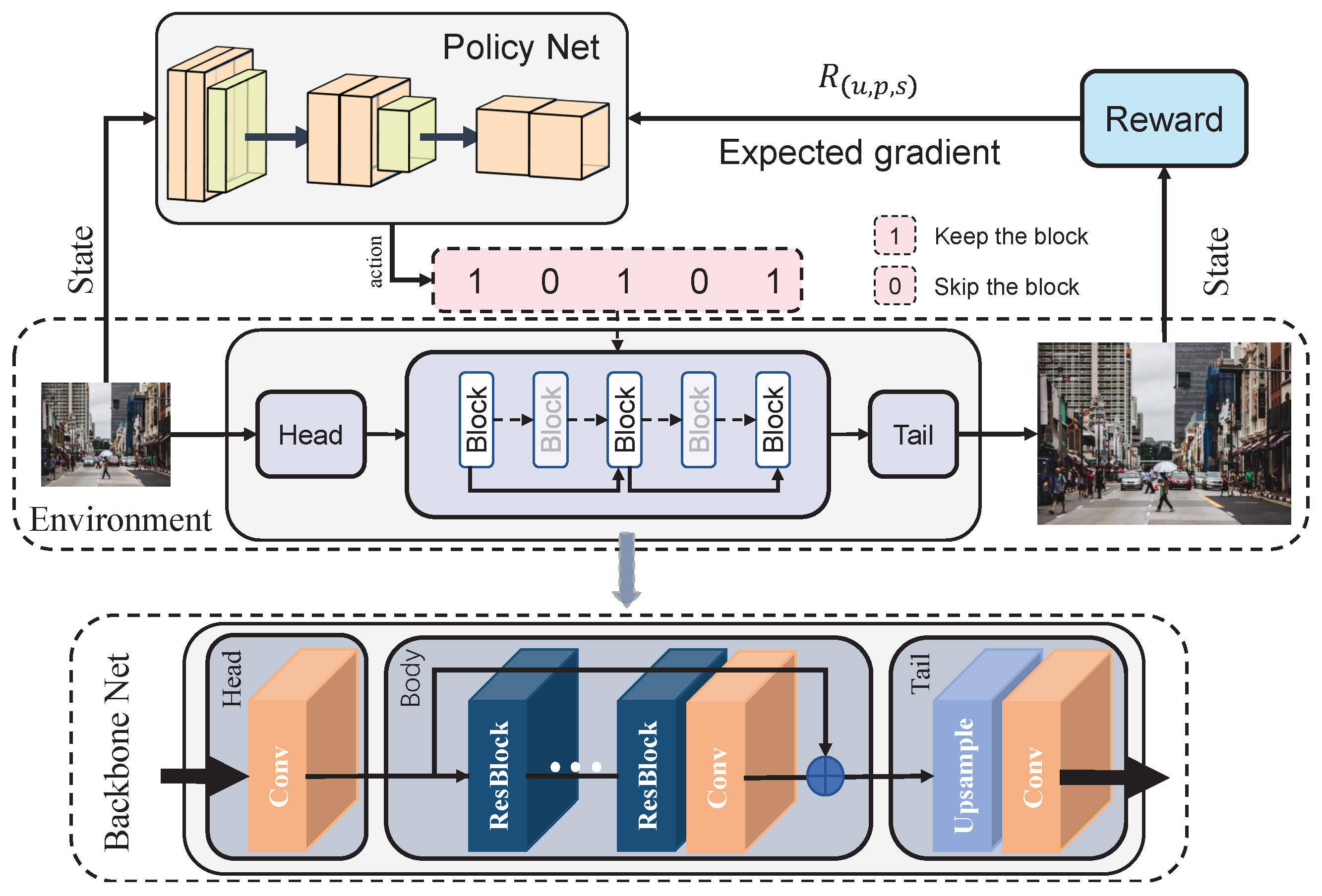
• We propose an agile super-resolution network via intelligent path selection (ASRN) for edge computing environments. ASRN adopts a dynamic path selection mechanism that utilizes a policy network to tailor computational pathways based on the real-time data.
• We introduced a smart reward mechanism in ASRN that has been ingeniously crafted to evaluate the policy network’s decisions. By comprehensively assessing the overall performance of the model and the effectiveness of current policy, it directs the policy network towards optimal choices, thereby marking a significant advancement for super-resolution applications in edge-computing scenarios.
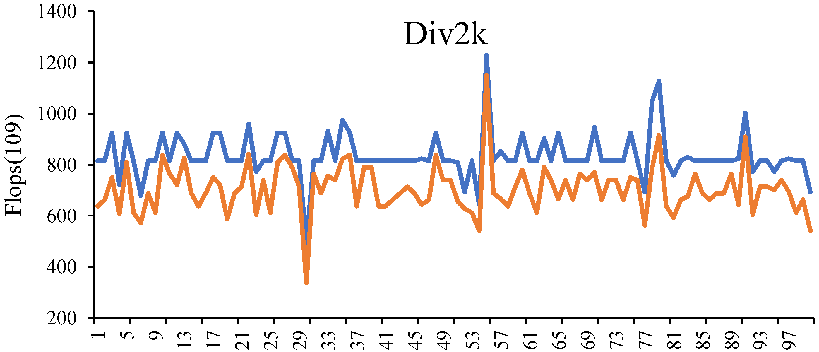
• Our extensive experiments across a variety of datasets confirmed the effectiveness of the proposed ASRN. In particular, on the Div2k dataset [20], we reduced the average number of residual blocks by 15.88% and the computational complexity (FLOPS) by 15.68% while maintaining performance close to baseline.

2. Related Work

2.1. Super-Resolution Technology

The development of super-resolution technology commenced with early interpolation-based methods, which primarily utilized linear techniques [21,22] to enhance image resolution. However, these methods often led to blurred images that lacked detail. The field experienced a significant transition with the advent of deep learning, particularly with the introduction of convolutional neural networks (CNNs) [23]. CNNs revolutionized super-resolution by enabling more complex and accurate image reconstruction, significantly improving the quality of upsampled images. This era also saw the integration of advanced techniques such as generative adversarial networks (GANs) [24], which introduced a competitive aspect to model training, resulting in sharper and more realistic images. Attention mechanisms [25,26], another significant advancement, allowed models to focus on specific image regions, enhancing detail where most needed. Ongoing advancements in the field are characterized by the exploration of novel deep learning architectures [27] and loss functions [28] that are aimed at enhancing the precision of super-resolution outputs.

2.2. Deep Learning Applications in Edge Computing

Edge computing presents a unique set of challenges for deep learning applications, primarily due to limitations in computational capacity and memory. The focus thus has shifted towards developing models that are not only lightweight but also are capable of achieving real-time performance. This is particularly critical for applications like video surveillance, autonomous driving, and real-time data analysis. The recent progress in this domain is to train models that are efficient both in terms of size and computational speed while not compromising on performance. Techniques like model quantization and network pruning [29,30] have been pivotal to achieving these goals. There is also an increasing trend towards designing custom hardware accelerators [31,32] that are specifically optimized for running deep learning models in resource-limited environments. This progress make edge computing a viable platform for advanced deep learning applications.

2.3. Lightweight Model Techniques

Efficient deployment of deep learning models on edge devices necessitates the reduction of their computational resource requirements without loss in performance. Lightweight model techniques are pivotal to achieving this by compressing and accelerating models while retaining their model performance. Each technique adopts a unique approach to tackle the challenges of limited resources:

Model Pruning: Pruning is a technique that reduces the complexity of neural networks by removing less important parameters or connections. It effectively reduces the model size and computational load without significantly impacting performance. Existing pruning methods now include structured pruning (removing entire neurons, channels, or layers) [33,34,35] and unstructured pruning (eliminating individual weights) [36]. Dynamic pruning, which adapts network complexity in real-time based on input data, is also promising.

Quantization: Quantization involves reducing the bit-size of model parameters, thereby lowering the model’s storage and computational demands. This process often converts floating-point parameters into fixed-point formats. The latest trends include mixed precision quantization [37,38], which applies different bit-widths to different parts of the network. Integration with other model compression techniques, such as pruning [39], enhances overall efficiency.

Knowledge Distillation: Knowledge distillation is a compression technique whereby a smaller model (student) learns to replicate the behavior of a larger model (teacher). The student model captures the essential information from the teacher, resulting in a compact yet effective version. Beyond the classic teacher–student setup, mutual learning [40,41] among multiple networks and cross-modal distillation [42,43] have been explored. These methods allow leveraging diverse data modalities and unlabeled data to improve the student model’s generalization.

Low-Rank Factorization: Low-rank factorization involves reducing the number of parameters in a model by decomposing large weight matrices into lower-rank approximations. This technique is particularly effective for reducing redundancies in convolutional layers. The focus is tensor decomposition methods like Candecomp/Parafac(CP) [44,45] and Tucker decompositions [46,47] for convolutional layers. These approaches maintain model performance while significantly reducing the parameter count.

Compared to existing lightweight model techniques, our proposed ASRN method demonstrates significant advantages. By adjusting a single hyperparameter, ASRN allows for flexible control over model performance, enabling efficient super-resolution processing in edge computing environments. Long et al. [48] also propose a dynamic path selection method by considering both the inference speed and the PSNR metric. This approach, however, overlooks the texture and structural integrity of the images evaluated by the SSIM metric. The proposed ASRN further improves Long’s work by taking the SSIM of the images into consideration when choosing the inference path: thus, effectively improving the quality of super-resolution performance. Our method achieves balanced optimization by considering not only the pixel fidelity but also the perceptual quality, thereby rectifying the bias and significantly enriching the model’s applicability to real-world scenarios. Unlike other one-time optimization techniques, ASRN supports dynamic adjustment, enabling the model to recover or further optimize its performance based on changes in available computational resources. This augmented flexibility and reversibility, now with a more comprehensive evaluation through PSNR and SSIM, are particularly crucial in edge computing scenarios faced with resource limitations and varying demands, proving the innovative and practical value of ASRN in the field of deep learning model optimization.

3. Agile Super-Resolution Network via Intelligent Path Selection

3.1. Overall Framework

This paper presents a network architecture designed to address the challenges of super-resolution tasks in edge computing environments. As illustrated in Figure 1, our network architecture comprises three key components: the backbone network, the policy network, and the reward mechanism. These components work collaboratively to enhance the efficiency and effectiveness of super-resolution processing, particularly in scenarios with limited computational resources.

3.2. Policy Network

In the proposed ASRN, the policy network plays a crucial role. Drawing on insights from previous studies analyzing ResNet, we recognized that skipping certain blocks within the network enhances inference efficiency without substantially affecting performance. This understanding has laid a vital foundation for our policy network design. The primary task of the policy network involves generating decision policies based on input data to determine the network architecture or operations to be executed during the inference process. Acting as an intelligent decision-maker, the policy network effectively selects the optimal inference paths according to the characteristics of the input data and the current computational resource limitations, thereby accelerating the inference process.

The policy generation process of the policy network is as follows:

$$m=f_p(x,w),$$

(1)

where $f_p$ represents the policy network parameterized by weights w, and m denotes the output policy corresponding to the input image x. We have carefully designed a lightweight policy network with far fewer parameters than the backbone network, ensuring minimal computational cost.

Different from the sampling policies in traditional reinforcement learning [49], the policy in our method is generated based on a k-dimensional Bernoulli distribution [50,51], expressed as:

$${\pi }_w\left(u\right|x)=\prod _{k=1}^{\mathrm{K}}{m}_k^{u_k}{(1-m_k)}^{1-u_k},$$

(2)

$$\mathbf{m}=(m_1,m_2,m_k),$$

(3)

where each element represents the decision to execute or skip the corresponding network block. With the help of the policy network, ASRN can flexibly adjust the network structure based on the complexity of the input images. This dynamic adjustment mechanism not only enhances the model’s inference speed but also ensures the quality of super-resolution images in resource-limited edge computing environments.

3.2.1. Design Principles of the Policy Network

The policy network in ASRN is grounded in deep reinforcement learning principles and continuously refines decision quality through iterative learning and optimization. Adopting a lightweight architecture—specifically, a simplified ResNet variant with three blocks—substantially reduces parameter count compared to the backbone network, ensuring effective decision-making without overburdening the inference process.

This pivotal component of ASRN comprises three ResNet blocks that are responsible for processing low-resolution images and generating a binary vector representing the policy. Dynamically aligning with the backbone network’s block quantity, this binary vector activates specific ResNet blocks during super-resolution, streamlining the inference path.

3.2.2. Policy Generation Process

Policy generation is based on a k-dimensional Bernoulli distribution that is calculated using Equations (2) and (3). Each element of the policy vector represents the decision to execute or skip a corresponding network block. This method enables the policy network to dynamically adjust the inference path according to different input data characteristics and resource limitations.

3.2.3. Collaboration of the Policy Network with the Backbone Network

The policy network does not operate independently but works closely with the backbone network. It intelligently adjusts the execution path of the backbone network based on the complexity of the input data. For instance, for relatively simple images, the policy network may choose a shorter path, skipping some unnecessary network blocks to accelerate processing.

3.2.4. Adaptability to Application Scenarios

We further explore the performance of the policy network in different application scenarios, such as processing high-resolution traffic surveillance images on resource-limited edge devices. In these scenarios, the policy network effectively adapts to various challenges, such as limited computational power and urgent inference time requirements.

Through this in-depth analysis, we demonstrate the key role of the policy network within the ASRN framework and how it supports the efficient execution of super-resolution tasks. This comprehensive and detailed discussion highlights the innovativeness and practical value of our research.

3.3. Reward Mechanism

To optimize the training process of the policy network, we employed reinforcement learning methods. In this process, the policy network makes decisions at each step of inference based on the actions chosen by the current policy. The performance of these decisions is evaluated through a carefully designed reward mechanism. The significance of the reward mechanism lies in its direct guidance for the policy network to choose optimal operations that simultaneously enhance inference speed and maintain super-resolution quality. Through this continuous optimization process, the policy network progressively becomes more intelligent and capable of generating increasingly effective inference policies.

The following reward function is defined for a backbone network with k residual blocks:

$$R_{(u,p,s)}=\left\{\begin{array}{cc}\frac{p-t}{\left(1-s\right){\left(\frac{\left|u\right|}{k}\right)}^2}ifp-t>0\hfill & \\ & \\ -\gamma else\hfill \end{array}\right.,$$

(4)

where u is a policy vector composed of binary values, where 1 represents the retention of the corresponding residual block, and 0 indicates skipping it. The dimension of the vector u is k, which is the total number of residual blocks in the network. The expression ${\left(\frac{\left|u\right|}{k}\right)}^2$ quantifies the degree to which individual blocks are incorporated into the overall network architecture. The variables s and p represent the performance evaluation results of the backbone network after applying the policy: specifically, they are the structural similarity index (SSIM) and the peak signal-to-noise ratio (PSNR), respectively, where $0<s<1$. The variable t is a critical hyperparameter that represents a threshold value we set to determine the application of rewards or penalties. Its specific value varies based on the employed evaluation method and the range of p (PSNR). When $p-t>0$, it indicates that the applied policy is effective, and thus, we provide a reward. This reward is directly proportional to the performance evaluation results after using the policy and inversely proportional to the number of residual blocks used. That is, better performance and fewer blocks used lead to larger rewards. Conversely, when $p-t\le 0$, it indicates that the policy is not effective, and we impose a penalty using the parameter $\gamma$.

In this way, the reward mechanism enables the policy network to more accurately adjust inference paths for samples of varying complexity, optimizing the performance and efficiency of the entire network.

3.4. Optimization of the Policy Network

In the proposed ASRN, special attention was given to the optimization policy of the policy network. Employing reinforcement learning methods, the policy network generates specific policies for each test sample with the aim of enhancing inference efficiency while maintaining super-resolution quality.

The optimization objective in Equation (5) is formulated to maximize the expected reward, which is expressed as

$$J\left(\theta \right)={\mathbb{E}}_{{\pi }_{\theta }}[R(s,a)],$$

where $J\left(\theta \right)$ represents the optimization objective with respect to policy parameters $\theta$, $R(s,a)$ denotes the reward for state s and action a, and ${\pi }_{\theta }$ is the policy under parameters $\theta$. This formulation guides the policy network to efficiently manage computational resources while enhancing or maintaining the quality of super-resolution. In accordance with the principles of reinforcement learning, the policy network updates its strategy based on the feedback loop of actions and rewards, iteratively improving its path selection decisions. This mechanism is akin to the exploration–exploitation trade-off, where the policy network explores various inference paths, learns from their performance outcomes, and exploits the knowledge to make more efficient decisions over time.

3.4.1. Optimization Objective

Our objective in this study is to maximize the expected value J to derive the optimal policy for the backbone model. Mathematically, this objective is expressed as:

$$J=E_{u\sim {\pi }_W}[R(u,p,s)].$$

(5)

This formula is in line with our goal of finding the most effective policy for super-resolution tasks. Through this methodological approach, the policy network continuously learns and improves across iterations, enabling the generation of more effective inference paths for the backbone network.

3.4.2. Application of Gradient Optimization Techniques

To optimize Equation (5), we employed gradient optimization techniques, as referenced in [52]. This involved substituting Equation (2) into Equation (5) to derive the optimization formulation for J. However, due to the non-differentiability of Equation (6), we resorted to the Monte Carlo [53,54] sampling method as an approximation technique to estimate the gradient of J. This approximation was achieved by using all available samples within a given mini-batch. Gradient optimization is mathematically represented as follows:

$$\begin{array}{cc}\hfill V_{\theta }J& =E[R(u,p,s){\nabla }_{\theta }\log {ß}_{\theta }\left(u\right|x)]\hfill \\ \hfill & =\mathrm{E}[R(u,p,s){\nabla }_{\theta }\log \sum _{k=1}^{\mathrm{K}}{m}_k^{u_k}{(1-m_k)}^{1-u_k}]\hfill \\ \hfill & =\mathrm{E}[R(u,p,s){\nabla }_{\theta }\sum _{k=1}^{\mathrm{K}}log[m_k^{u_k}{(1-m_k)}^{1-u_k}]].\hfill \end{array}$$

(6)

3.4.3. Policy for Reducing Variance

While the gradient approximation is unbiased, it is prone to cause significant variance, as noted in [49]. To mitigate this issue, we introduced a self-critical baseline $R(\widehat{u},p)$ as a technique for variance reduction. This approach leads to the reformulation of Equation (6). The modified equation for gradient optimization, incorporating the self-critical baseline, is represented as follows:

$${\nabla }_{\theta }\mathrm{J}=\mathrm{E}[\mathrm{R}(\mathrm{u},\mathrm{p},\mathrm{s})-\mathrm{R}(\widehat{\mathrm{u}},\mathrm{p},\mathrm{s})]{\nabla }_{\theta }\sum _{k=1}^{\mathrm{K}}log\left[m_k^{u_k}{(1-m_k)}^{1-u_k}\right].$$

(7)

In Equation (7), $\widehat{u}$ represents the most likely policy under the current policy probability $m_k$. Here, the binary variable $u_i=1$ when $m_i>0.5$; conversely, when $m_i\le 0.5$, $u_i=0$. This reformulation helps to reduce the variance of the gradient estimation, thereby enhancing the reliability of the optimization process.

3.4.4. Incentive Mechanism for Policy Exploration

To encourage the exploration of more optimal policies by the policy network and reduce the risk of policy saturation, we introduced the parameter $\alpha$. This parameter is used to adjust the range of the policy vector $m^{\prime }$, ensuring it stays within the interval $[1-\alpha ,\alpha ]$. Such an adjustment is crucial to maintain the policy network’s exploratory capabilities while preventing it from straying too far from the boundaries of desirable policies. The adjustment of the policy vector is mathematically expressed as:

$$m^{\prime }=\alpha m+(1-\alpha )(1-m).$$

(8)

3.4.5. Parameter Sensitivity Analysis

We evaluated the sensitivity of the ASRN model on the Set5 dataset to the reward function parameters $\gamma$ (gamma) and t (threshold) and report the results in

Table 1. Sensitivity analysis of reward function parameters.

$\mathit{\gamma }$	t	PSNR	Blocks Used
−100	30	37.364	28
−50	30	37.380	27
−10	30	37.450	26
−100	100	37.415	30
−100	50	37.402	29
−100	10	37.421	25

. The optimal settings of $\gamma$ = −10 and t = 30 yield the highest PSNR of 37.450 while using only 26 blocks, indicating that precise parameter tuning can significantly enhance super-resolution quality. On the contrary, extreme values like $\gamma$ = −100 with t = 100 or t = 10, despite maintaining competitive PSNR levels, require using more blocks, reducing network efficiency.

Intermediate values such as $\gamma$ = −50 and t = 30 achieve a PSNR of 37.380 and use 27 blocks, showing the sensitivity of the ASRN model to its reward function parameters and emphasizing the importance of careful calibration to strike an optimal balance between super-resolution quality and computational efficiency.

In summary, sensitivity analysis, as depicted in Table 1, is crucial for optimizing the performance of the ASRN model, particularly in resource-constrained edge computing environments, and enables a strategic balance between high-quality super-resolution and efficient computational usage.

By employing these optimization policies, the ASRN demonstrates impressive performance and efficiency across various datasets and application scenarios. This section is dedicated to exploring the optimization process of the policy network and underscoring its vital contribution to enhancing the efficiency of the super-resolution network model. The strategic balance achieved by this mechanism facilitates the discovery of effective inference policies, thereby augmenting the model’s overall robustness and adaptability in different computing environments.

4. Experiments

In this section, we provide a detailed account of the integration of the policy network into the EDSR [55] backbone network and assess the effectiveness of our approach across five different datasets. Our primary goal is to significantly reduce the inference time of the network while maintaining super-resolution performance, with a particular focus on edge devices limited by storage and computational resources.

This comprehensive evaluation aims to demonstrate the practical applicability and efficiency of our method in diverse scenarios, highlighting its potential in addressing the challenges faced in edge computing environments, where resource optimization is crucial.

4.1. Experimental Setup

4.1.1. Dataset

The Div2k dataset is a widely used benchmark in super-resolution research and comprises 800 high-quality training images and 100 validation images. Different super-resolution tasks share some similarities in pixel statistics. Therefore, based on the philosophy of transfer learning, we initialize the parameters through a model pretrained on the Div2k training set (just like initializing the classification models through a model pretrained on ImageNet [56]). To comprehensively assess the effectiveness and adaptability of our method, tests were conducted not only on the Div2k validation set but also on four additional benchmark datasets, including Set5 [57], Set14 [58], B100 [59], and Urban100 [60]. These experiments were designed to validate the generalization ability of the policy network across different image characteristics and real-world scenarios.

4.1.2. Network Architecture Components

We selected the EDSR network as the backbone for our super-resolution task; the EDSR network consists of a head, body, and tail, with the body comprising 32 residual blocks. The network model was trained from scratch using the first 800 images from the Div2k dataset, ensuring that the model could adequately learn and adapt to a variety of image features.

We use a ResNet with three blocks (equivalently, ResNet-8), with the aim of minimizing the computational overhead introduced. This lightweight design allows the policy network to effectively support the backbone network without becoming a computational bottleneck. Its smaller scale compared to the backbone network ensures that it plays a supportive role in our overall approach, allowing us to allocate more computational resources to the actual super-resolution task while benefiting from the intelligent guidance provided by the policy network. During training, we employ the ADAM optimizer with a learning rate of 1 ×${10}^{-4}$ and betas of (0.9, 0.999). To enhance convergence and stability, step decay on the learning rate is utilized, with a decay interval of 200 epochs and a decay factor of 0.5. Notably, the policy network’s training integrates reinforcement learning, with rewards derived from the backbone network’s output, ensuring alignment between super-resolution quality and computational efficiency.

Next, we will present the experimental results on these datasets and analyze the performance of our method on different datasets and with different settings. Specifically, we will focus on discussing the adaptability of the policy network to various scenarios and its ability to balance inference speed and image quality.

4.2. Balancing Speed and Quality

In this study, we focused particularly on balancing the speed and image quality of the super-resolution model. To this end, we compared the performance of our ASRN model with the original EDSR model and other popular super-resolution models such as A+ [61], SRCNN [62], VDSR [63], and SRResNet [64].

4.2.1. Performance Comparison Analysis

Upon analysis of Figure 2, Figure 3 and Figure 4, we illustrate the dynamic selection process employed by our policy network across different datasets, highlighting its capacity to adjust the computational depth in accordance with the complexity of input images. This process emphasizes the policy network’s adaptability, ensuring computational efficiency and maintaining super-resolution quality. For simpler images, fewer neural network blocks are required, whereas complex images necessitate a more extensive computational effort.

Further insights are provided in

Table 2. Representative examples of FLOPS (10⁹) reduction in B100 dataset.

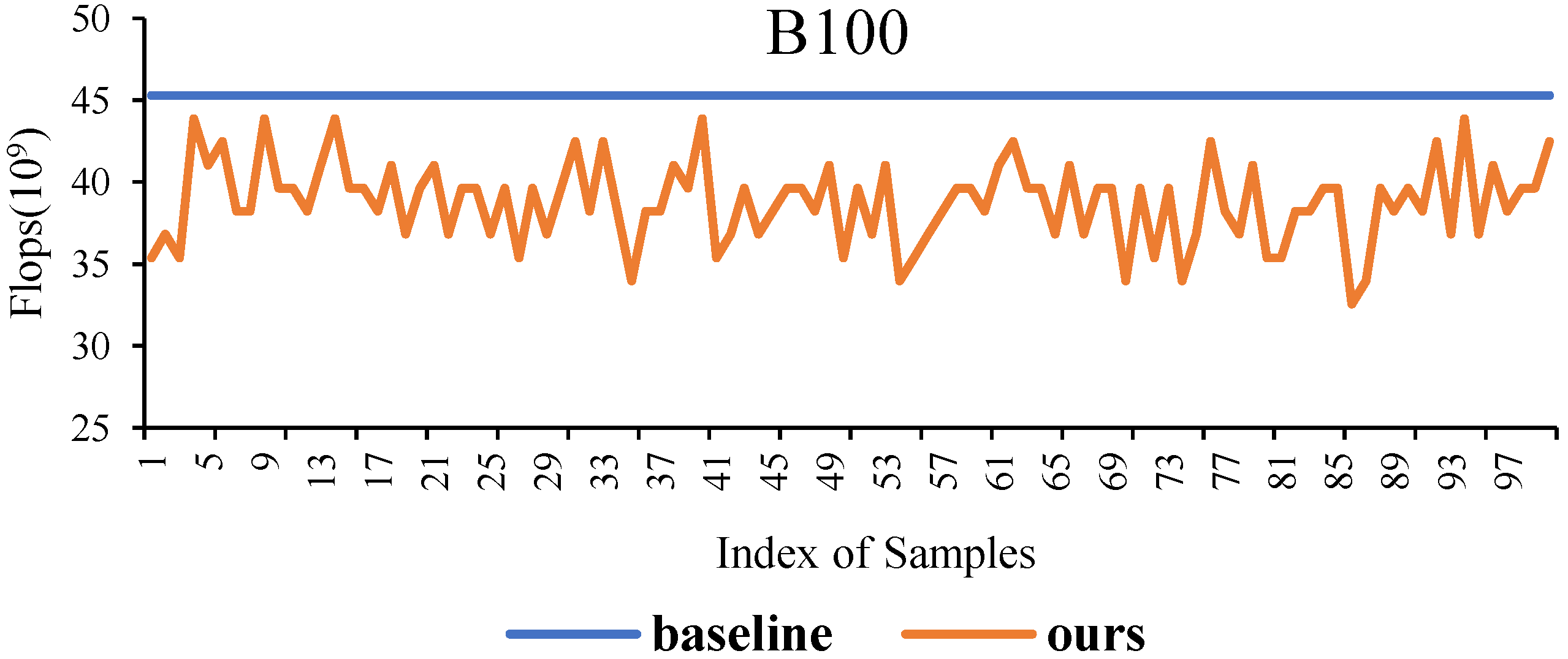
Image ID	Baseline	Ours	Reduction	Speedup
33	45.3	42.47	2.83	6.35%
38	45.3	41.05	4.25	9.38%
43	45.3	39.64	5.66	12.49%
74	45.3	33.97	11.33	25.00%
35	45.3	32.56	12.74	28.12%

,

Table 3. Representative examples of FLOPS (10⁹) reduction in Urban100 dataset.

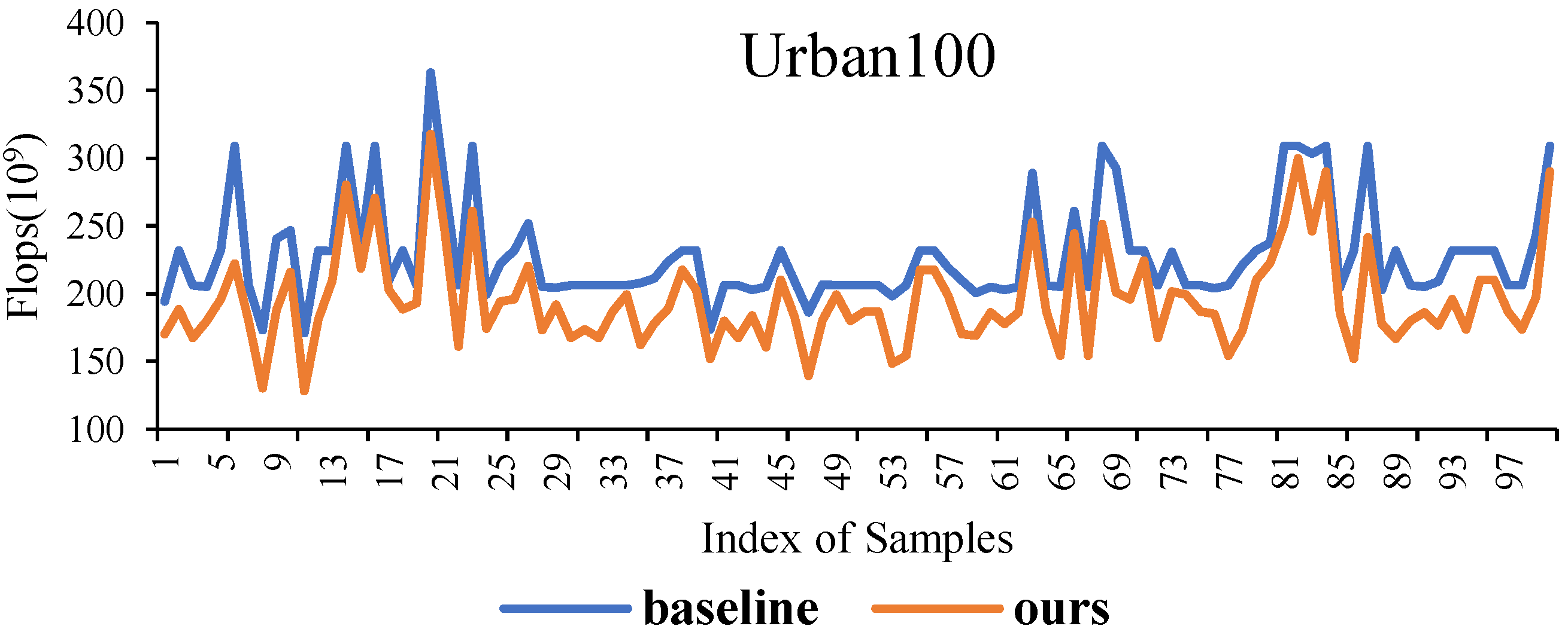
Image ID	Baseline	Ours	Reduction	Speedup
43	202.94	183.91	19.03	9.38%
50	205.96	180.21	25.75	12.50%
58	209.58	170.28	39.3	18.75%
67	205.35	154.01	51.34	25.00%
86	231.93	152.2	79.73	34.38%

and

Table 4. Representative examples of FLOPS (10⁹) reduction in Div2k dataset.

Image ID	Baseline	Ours	Reduction	Speedup
10	924.09	837.46	86.63	9.37%
42	815.80	662.84	152.96	18.75%
78	1046.82	785.11	261.71	25.00%
19	815.80	586.35	229.54	28.13%
30	490.92	337.51	153.41	31.25%

, which detail the FLOPS reduction for representative examples, demonstrating our approach’s effectiveness at varying degrees of model simplification. This approach underscores our model’s flexibility in balancing the demand for high-quality super-resolution against the constraints of limited computational resources, marking a significant advancement in the field of super-resolution within edge computing environments.

By analyzing

Table 5. Analysis of our method regarding usage blocks and flops across various datasets.

Evaluation (avg.)		Set5	Set14	B100	Urban100	Div2k
PSNR/SSIM	Baseline Ours	38.11/0.9601 38.02/0.9586	33.92/0.9195 33.74/0.9166	32.32/0.9013 32.24/0.9018	32.93/0.9351 32.28/0.9274	35.03/0.9695 34.73/0.9676
BLOCKS	Baseline Ours Speedup	32 28.99 9.41%	32 28.13 12.09%	32 27.48 14.14%	32 27.46 14.19%	32 26.90 15.93%
FLOPS (109)	Baseline Ours Speedup	33.47 30.33 9.37%	67.86 58.64 13.58%	45.3 38.86 14.21%	228.59 195.70 14.39%	836.09 704.57 15.73%

, it is evident that there is an average enhancement in inference speed of 9.41% to 15.93% across various datasets without any significant alteration in image quality following super-resolution processing. This observation leads us to further explore the comparative performance of different super-resolution models.

4.2.2. Significant Reduction in Inference Time

By analyzing

Table 6. Comparative analysis of experimental results (PSNR and SSIM) on different datasets. (Block utilization rates for our model are: Set5 90.59%, Set14 87.91%, B100 85.86%, Urban100 85.81%, and Div2k 84.07%).

Dataset	Block Usage	Scale	Bicubic		A+		SRCNN		VDSR		Ours		EDSR
			PSNR	SSIM	PSNR	SSIM	PSNR	SSIM	PSNR	SSIM	PSNR	SSIM	PSNR	SSIM
Set5	90.59%	X2	33.66	0.9229	36.54	0.9544	36.66	0.9542	37.53	0.9587	38.02	0.9586	38.11	0.9601
		X3	30.39	0.8682	32.58	0.9088	32.75	0.9090	33.66	0.9213	34.59	0.9263	34.65	0.9282
		X4	28.42	0.8104	30.28	0.8603	30.48	0.8628	31.35	0.8838	32.37	0.8945	32.46	0.8968
Set14	87.91%	X2	30.24	0.8688	32.28	0.9056	32.42	0.9063	33.03	0.9124	33.74	0.9166	33.92	0.9195
		X3	27.55	0.7742	29.13	0.8188	29.28	0.8209	29.77	0.8314	30.34	0.8426	30.52	0.8462
		X4	26.00	0.7027	27.32	0.7491	27.49	0.7503	28.01	0.7674	28.64	0.7843	28.80	0.7876
B100	85.86%	X2	29.56	0.8431	31.21	0.8863	31.36	0.8879	31.90	0.8960	32.24	0.9018	32.32	0.9013
		X3	27.21	0.7385	28.29	0.7835	28.41	0.7863	28.82	0.7976	29.08	0.8074	29.25	0.8093
		X4	25.96	0.6675	26.82	0.7087	26.90	0.7101	27.29	0.7251	27.62	0.7363	27.71	0.7420
Urban100	85.81%	X2	26.88	0.8403	29.20	0.8938	29.50	0.8946	30.76	0.9140	32.28	0.9274	32.93	0.9351
		X3	24.46	0.7349	26.03	0.7973	26.24	0.7989	27.14	0.8279	28.33	0.8562	28.80	0.8653
		X4	23.14	0.6577	24.32	0.7183	24.52	0.7221	25.18	0.7524	26.24	0.7931	26.64	0.8033
Div2k	84.07%	X2	31.01	0.9393	32.89	0.9570	33.05	0.9581	33.66	0.9625	34.73	0.9676	35.03	0.9695
		X3	28.22	0.8906	29.50	0.9116	29.64	0.9138	30.09	0.9208	30.92	0.9307	31.26	0.9340
		X4	26.66	0.8521	27.70	0.8736	27.78	0.8753	28.17	0.8841	28.97	0.8987	29.25	0.9017

, it is observed that our ASRN model consistently surpasses other models with regard to super-resolution performance across all datasets. Despite a marginal decrement in performance metrics, the model significantly reduces computational complexity (FLOPS), thereby directly speeding up the inference time. This noteworthy reduction in computational overhead not only demonstrates a groundbreaking methodology for the efficient execution of super-resolution tasks but also highlights the model’s crucial role in edge computing settings, where computational resources and storage capacities are limited. Such outcomes offer new possibilities for efficiently handling super-resolution tasks in environments that demand swift and resource-conscious processing.

Our analyses further reveal a direct correlation between image complexity and the computational efficiency achieved by ASRN. Specifically, Figure 5, Figure 6 and Figure 7 illustrate that simpler images necessitate fewer processing blocks, while more complex images require a greater number. This adaptive behavior underscores the ASRN’s capacity to dynamically adjust its processing policy according to the image’s complexity, ensuring optimal resource utilization and faster inference speeds across varied scenarios.

4.2.3. Scalability Testing

We conducted scalability tests of ASRN on edge computing devices with different computational capabilities. On a Texas Instruments MSP432P401R, ASRN reduced the average inference time from 156.490 s to 146.159 s, while on an ARM Cortex-M7, the inference time decreased from 62.596 s to 58.464 s. From the data presented in

Table 7. Texas Instruments MSP432P401R: 100 MHz (inference time).

	Data 0	Data 1	Data 2	Data 3	Data 4	Average
Baseline	384.626 s	106.37 s	92.334 s	96.162 s	102.96 s	156.490 s
Ours	370.942 s	92.994 s	73.700 s	90.772 s	102.388 s	146.159 s

and

Table 8. ARM Cortex-M7: 250 MHz (inference time).

	Data 0	Data 1	Data 2	Data 3	Data 4	Average
Baseline	153.850 s	42.548 s	36.934 s	38.465 s	41.184 s	62.596 s
Ours	148.377 s	37.198 s	29.480 s	36.309 s	40.955 s	58.464 s

, these results demonstrate the scalability of ASRN across different edge devices, further validating its effectiveness in diverse edge computing environments and emphasizing its potential to enhance super-resolution tasks across a variety of computing resources.

4.2.4. Application Insights and Future Perspectives

The experimental results proved the effectiveness of the policy network for optimizing resource usage. With minimal or no degradation in performance, ASRN achieved a significant reduction in computational load and storage requirements. This provides a practical solution for super-resolution applications on edge devices, especially in scenarios with strict requirements for inference speed and efficiency.

Furthermore, our work offers valuable insights for future research and applications in the field of edge computing, particularly for resource optimization and real-time data processing. ASRN demonstrates the tremendous potential of super-resolution technology in edge computing environments.

In summary, our research has not only made significant technical progress but also provides important references and directions for future studies and applications in similar fields.

5. Conclusions

In this paper, we proposed an agile super-resolution network via intelligent path selection (ASRN): an efficient super-resolution model tailored to edge computing environments. ASRN aims to significantly reduce the inference time of super-resolution network models on edge devices while maintaining high-quality performance. By incorporating a policy network, ASRN dynamically selects the most efficient inference paths based on input data and available computational resources. The key to our approach is the intelligent reward function, which refines the decision-making process by evaluating the effectiveness of chosen paths, thus optimizing both the speed and quality of super-resolution outcomes.

Our research not only demonstrates the effectiveness of the policy network for handling super-resolution tasks but also reveals its extensive potential for accelerating inference processes across various edge device applications. The significant technical progress made by ASRN offers fresh perspectives and possibilities for future research and practical applications in this rapidly evolving field.

References

- Lugmayr, A.; Danelljan, M.; Timofte, R. Unsupervised Learning for Real-World Super-Resolution. In Proceedings of the 2019 IEEE/CVF International Conference on Computer Vision Workshop (ICCVW), Seoul, Republic of Korea, 27–28 October 2019; IEEE: Piscataway, NJ, USA, 2019; pp. 3408–3416. [Google Scholar]
- Park, S.C.; Park, M.K.; Kang, M.G. Super-resolution image reconstruction: A technical overview. IEEE Signal Process. Mag. 2003, 20, 21–36. [Google Scholar] [CrossRef]
- Yue, L.; Shen, H.; Li, J.; Yuan, Q.; Zhang, H.; Zhang, L. Image super-resolution: The techniques, applications, and future. Signal Process. 2016, 128, 389–408. [Google Scholar] [CrossRef]
- He, K.; Zhang, X.; Ren, S.; Sun, J. Deep Residual Learning for Image Recognition. In Proceedings of the IEEE Conference on Computer Vision and Pattern Recognition, Las Vegas, NV, USA, 26 June–1 July 2016; pp. 770–778. [Google Scholar]
- Cheng, Y.; Wang, D.; Zhou, P.; Zhang, T. A survey of model compression and acceleration for deep neural networks. arXiv 2017, arXiv:1710.09282. [Google Scholar]
- Chen, Y.; Fan, H.; Xu, B.; Yan, Z.; Kalantidis, Y.; Rohrbach, M.; Yan, S.; Feng, J. Drop an Octave: Reducing Spatial Redundancy in Convolutional Neural Networks with Octave Convolution. In Proceedings of the IEEE/CVF International Conference on Computer Vision, Seoul, Republic of Korea, 27 October–2 November 2019; pp. 3435–3444. [Google Scholar]
- Ayinde, B.O.; Inanc, T.; Zurada, J.M. Redundant feature pruning for accelerated inference in deep neural networks. Neural Netw. 2019, 118, 148–158. [Google Scholar] [CrossRef] [PubMed]
- Li, H.; Kadav, A.; Durdanovic, I.; Samet, H.; Graf, H.P. Pruning filters for efficient convnets. arXiv 2016, arXiv:1608.08710. [Google Scholar]
- Polyak, A.; Wolf, L. Channel-level acceleration of deep face representations. IEEE Access 2015, 3, 2163–2175. [Google Scholar] [CrossRef]
- Yu, R.; Li, A.; Chen, C.F.; Lai, J.H.; Morariu, V.I.; Han, X.; Gao, M.; Lin, C.Y.; Davis, L.S. Nisp: Pruning Networks Using Neuron Importance Score Propagation. In Proceedings of the IEEE Conference on Computer Vision and Pattern Recognition, Salt Lake City, UT, USA, 18–23 June 2018; pp. 9194–9203. [Google Scholar]
- Wu, J.; Leng, C.; Wang, Y.; Hu, Q.; Cheng, J. Quantized convolutional neural networks for mobile devices. In Proceedings of the IEEE Conference on Computer Vision and Pattern Recognition, Las Vegas, NV, USA, 26 June–1 July 2016; pp. 4820–4828. [Google Scholar]
- Li, H.; De, S.; Xu, Z.; Studer, C.; Samet, H.; Goldstein, T. Training quantized nets: A deeper understanding. Adv. Neural Inf. Process. Syst. 2017, 30. [Google Scholar]
- Han, S.; Mao, H.; Dally, W.J. Deep compression: Compressing deep neural networks with pruning, trained quantization and huffman coding. arXiv 2015, arXiv:1510.00149. [Google Scholar]
- Ioannou, Y.; Robertson, D.; Shotton, J.; Cipolla, R.; Criminisi, A. Training cnns with low-rank filters for efficient image classification. arXiv 2015, arXiv:1511.06744. [Google Scholar]
- Sainath, T.N.; Kingsbury, B.; Sindhwani, V.; Arisoy, E.; Ramabhadran, B. Low-Rank Matrix Factorization for Deep Neural Network Training with High-Dimensional Output Targets. In Proceedings of the 2013 IEEE International Conference on Acoustics, Speech and Signal Processing, Vancouver, BC, Canada, 26–31 May 2013; IEEE: Piscataway, NJ, USA, 2013; pp. 6655–6659. [Google Scholar]
- Tai, C.; Xiao, T.; Zhang, Y.; Wang, X. Convolutional neural networks with low-rank regularization. arXiv 2015, arXiv:1511.06067. [Google Scholar]
- Chen, G.; Choi, W.; Yu, X.; Han, T.; Chandraker, M. Learning efficient object detection models with knowledge distillation. Adv. Neural Inf. Process. Syst. 2017, 30, 483. [Google Scholar]
- Hinton, G.; Vinyals, O.; Dean, J. Distilling the knowledge in a neural network. arXiv 2015, arXiv:1503.02531. [Google Scholar]
- Romero, A.; Ballas, N.; Kahou, S.E.; Chassang, A.; Gatta, C.; Bengio, Y. Fitnets: Hints for thin deep nets. arXiv 2014, arXiv:1412.6550. [Google Scholar]
- Timofte, R.; Agustsson, E.; Van Gool, L.; Yang, M.H.; Zhang, L. Ntire 2017 challenge on single image super-resolution: Methods and results. In Proceedings of the IEEE Conference on Computer Vision and Pattern Recognition Workshops, Honolulu, HI, USA, 21–26 July 2017; pp. 114–125. [Google Scholar]
- Zhang, K.; Tao, D.; Gao, X.; Li, X.; Xiong, Z. Learning multiple linear mappings for efficient single image super-resolution. IEEE Trans. Image Process. 2015, 24, 846–861. [Google Scholar] [CrossRef] [PubMed]
- Bevilacqua, M.; Roumy, A.; Guillemot, C.; Morel, M.L.A. Single-image super-resolution via linear mapping of interpolated self-examples. IEEE Trans. Image Process. 2014, 23, 5334–5347. [Google Scholar] [CrossRef] [PubMed]
- Ketkar, N.; Moolayil, J.; Ketkar, N.; Moolayil, J. Convolutional Neural Networks. In Deep Learning with Python: Learn Best Practices of Deep Learning Models with PyTorch; Apress: New York, NY, USA, 2021; pp. 197–242. [Google Scholar]
- Creswell, A.; White, T.; Dumoulin, V.; Arulkumaran, K.; Sengupta, B.; Bharath, A.A. Generative adversarial networks: An overview. IEEE Signal Process. Mag. 2018, 35, 53–65. [Google Scholar] [CrossRef]
- Guo, M.H.; Xu, T.X.; Liu, J.J.; Liu, Z.N.; Jiang, P.T.; Mu, T.J.; Zhang, S.H.; Martin, R.R.; Cheng, M.M.; Hu, S.M. Attention mechanisms in computer vision: A survey. Comput. Vis. Media 2022, 8, 331–368. [Google Scholar] [CrossRef]
- Burt, P.J. Attention Mechanisms for Vision in a Dynamic World. In Proceedings of the 9th International Conference on Pattern Recognition, Valletta, Malta, 22–24 February 2020; IEEE Computer Society: Piscataway, NJ, USA, 1988; pp. 977–978. [Google Scholar]
- Kawulok, M.; Benecki, P.; Piechaczek, S.; Hrynczenko, K.; Kostrzewa, D.; Nalepa, J. Deep learning for multiple-image super-resolution. IEEE Geosci. Remote. Sens. Lett. 2019, 17, 1062–1066. [Google Scholar] [CrossRef]
- Johnson, J.; Alahi, A.; Fei-Fei, L. Perceptual Losses for Real-Time Style Transfer and Super-Resolution. In Proceedings of the Computer Vision—ECCV 2016: 14th European Conference, Amsterdam, The Netherlands, 11–14 October 2016; Part II 14. Springer: Berlin/Heidelberg, Germany, 2016; pp. 694–711. [Google Scholar]
- Bai, S.; Chen, J.; Shen, X.; Qian, Y.; Liu, Y. Unified Data-Free Compression: Pruning and Quantization without Fine-Tuning. In Proceedings of the IEEE/CVF International Conference on Computer Vision, Paris, France, 2–6 October 2023; pp. 5876–5885. [Google Scholar]
- Shen, W.; Wang, W.; Zhu, J.; Zhou, H.; Wang, S. Pruning-and Quantization-Based Compression Algorithm for Number of Mixed Signals Identification Network. Electronics 2023, 12, 1694. [Google Scholar] [CrossRef]
- Zhang, S.; Sohrabizadeh, A.; Wan, C.; Huang, Z.; Hu, Z.; Wang, Y.; Cong, J.; Sun, Y.; Lin, Y. A Survey on Graph Neural Network Acceleration: Algorithms, Systems, and Customized Hardware. arXiv 2023, arXiv:2306.14052. [Google Scholar]
- Zeng, Z.; Sapatnekar, S.S. Energy-efficient Hardware Acceleration of Shallow Machine Learning Applications. In Proceedings of the 2023 Design, Automation & Test in Europe Conference & Exhibition (DATE), Antwerp, Belgium, 17–19 April 2023; IEEE: Piscataway, NJ, USA, 2023; pp. 1–6. [Google Scholar]
- Anwar, S.; Hwang, K.; Sung, W. Structured pruning of deep convolutional neural networks. Acm J. Emerg. Technol. Comput. Syst. (JETC) 2017, 13, 1–18. [Google Scholar] [CrossRef]
- He, Y.; Zhang, X.; Sun, J. Channel Pruning for Accelerating Very Deep Neural Networks. In Proceedings of the IEEE International Conference on Computer Vision, Venice, Italy, 22–29 October 2017; pp. 1389–1397. [Google Scholar]
- Lin, S.; Ji, R.; Yan, C.; Zhang, B.; Cao, L.; Ye, Q.; Huang, F.; Doermann, D. Towards Optimal Structured cnn Pruning via Generative Adversarial Learning. In Proceedings of the IEEE/CVF Conference on Computer Vision and Pattern Recognition, Long Beach, CA, USA, 15–20 June 2019; pp. 2790–2799. [Google Scholar]
- Liu, Z.; Sun, M.; Zhou, T.; Huang, G.; Darrell, T. Rethinking the value of network pruning. arXiv 2018, arXiv:1810.05270. [Google Scholar]
- Gholami, A.; Kim, S.; Dong, Z.; Yao, Z.; Mahoney, M.W.; Keutzer, K. A survey of quantization methods for efficient neural network inference. In Low-Power Computer Vision; Chapman and Hall/CRC: Boca Raton, FL, USA, 2022; pp. 291–326. [Google Scholar]
- Nagel, M.; Fournarakis, M.; Amjad, R.A.; Bondarenko, Y.; Van Baalen, M.; Blankevoort, T. A white paper on neural network quantization. arXiv 2021, arXiv:2106.08295. [Google Scholar]
- Xu, S.; Huang, A.; Chen, L.; Zhang, B. Convolutional Neural Network Pruning: A Survey. In Proceedings of the 2020 39th Chinese Control Conference (CCC), Shenyang, China, 27–29 July 2020; IEEE: Piscataway, NJ, USA, 2020; pp. 7458–7463. [Google Scholar]
- Zhang, Y.; Xiang, T.; Hospedales, T.M.; Lu, H. Deep mutual learning. In Proceedings of the IEEE Conference on Computer Vision and Pattern Recognition, Salt Lake City, UT, USA, 18–23 June 2018; pp. 4320–4328. [Google Scholar]
- Shen, T.; Zhang, J.; Jia, X.; Zhang, F.; Huang, G.; Zhou, P.; Kuang, K.; Wu, F.; Wu, C. Federated mutual learning. arXiv 2020, arXiv:2006.16765. [Google Scholar]
- Gupta, S.; Hoffman, J.; Malik, J. Cross Modal Distillation for Supervision Transfer. In Proceedings of the IEEE Conference on Computer Vision and Pattern Recognition, Las Vegas, NV, USA, 26 June–1 July 2016; pp. 2827–2836. [Google Scholar]
- Afouras, T.; Chung, J.S.; Zisserman, A. Asr is all you need: Cross-modal distillation for lip reading. In Proceedings of the ICASSP 2020—2020 IEEE International Conference on Acoustics, Speech and Signal Processing (ICASSP), Las Vegas, NV, USA, 26 June–1 July 2020; IEEE: Piscataway, NJ, USA, 2020; pp. 2143–2147. [Google Scholar]
- Liu, K.; Da Costa, J.P.C.; So, H.C.; Huang, L.; Ye, J. Detection of number of components in CANDECOMP/PARAFAC models via minimum description length. Digit. Signal Process. 2016, 51, 110–123. [Google Scholar] [CrossRef]
- Phan, A.H.; Tichavskỳ, P.; Cichocki, A. CANDECOMP/PARAFAC decomposition of high-order tensors through tensor reshaping. IEEE Trans. Signal Process. 2013, 61, 4847–4860. [Google Scholar] [CrossRef]
- Jang, J.G.; Kang, U. D-Tucker: Fast and Memory-Efficient Tucker Decomposition for Dense Tensors. In Proceedings of the 2020 IEEE 36th International Conference on Data Engineering (ICDE), Dallas, TX, USA, 20–24 April 2020; IEEE: Piscataway, NJ, USA, 2020; pp. 1850–1853. [Google Scholar]
- Ahmadi-Asl, S.; Abukhovich, S.; Asante-Mensah, M.G.; Cichocki, A.; Phan, A.H.; Tanaka, T.; Oseledets, I. Randomized algorithms for computation of Tucker decomposition and higher order SVD (HOSVD). IEEE Access 2021, 9, 28684–28706. [Google Scholar] [CrossRef]
- Jia, L.; Hu, Y.; Tian, X.; Luo, W. Fast Super-Resolution Network via Dynamic Path Selection. In Proceedings of the 2023 International Conference on Image Processing, Computer Vision and Machine Learning (ICICML), Chengdu, China, 3–5 November 2023; IEEE: Piscataway, NJ, USA, 2023; pp. 1093–1099. [Google Scholar]
- Sutton, R.S.; Barto, A.G. The reinforcement learning problem. In Reinforcement learning: An introduction; MIT Press: Cambridge, MA, USA, 1998; pp. 51–85. [Google Scholar]
- Barthélemy, J.; Suesse, T. mipfp: An R package for multidimensional array fitting and simulating multivariate Bernoulli distributions. J. Stat. Softw. 2018, 86. [Google Scholar] [CrossRef]
- Fraiman, R.; Moreno, L.; Ransford, T. A quantitative Heppes theorem and multivariate Bernoulli distributions. J. R. Stat. Soc. Ser. B Stat. Methodol. 2023, 85, 293–314. [Google Scholar] [CrossRef]
- Ratliff, N.; Zucker, M.; Bagnell, J.A.; Srinivasa, S. CHOMP: Gradient Optimization Techniques for Efficient Motion Planning. In Proceedings of the 2009 IEEE International Conference on Robotics and Automation, Kobe, Japan, 12–17 May 2009; IEEE: Piscataway, NJ, USA, 2009; pp. 489–494. [Google Scholar]
- Metropolis, N.; Ulam, S. The monte carlo method. J. Am. Stat. Assoc. 1949, 44, 335–341. [Google Scholar] [CrossRef] [PubMed]
- Bielajew, A.F. History of monte carlo. In Monte Carlo Techniques in Radiation Therapy; CRC Press: Boca Raton, FL, USA, 2021; pp. 3–15. [Google Scholar]
- Lim, B.; Son, S.; Kim, H.; Nah, S.; Mu Lee, K. Enhanced Deep Residual Networks for Single Image Super-Resolution. In Proceedings of the IEEE Conference on Computer Vision and Pattern Recognition Workshops, Honolulu, HI, USA, 21–26 July 2017; pp. 136–144. [Google Scholar]
- Krizhevsky, A.; Sutskever, I.; Hinton, G.E. ImageNet Classification with Deep Convolutional Neural Networks. Adv. Neural Inf. Process. Syst. 2012, 25. [Google Scholar] [CrossRef]
- Bevilacqua, M.; Roumy, A.; Guillemot, C.; Alberi-Morel, M.L. Low-Complexity Single-Image Super-Resolution Based on Nonnegative Neighbor Embedding. In Proceedings of the 23rd British Machine Vision Conference (BMVC), Surrey, UK, 3–7 September 2012. [Google Scholar]
- Zeyde, R.; Elad, M.; Protter, M. On Single Image Scale-Up Using Sparse-Representations. In Proceedings of the Curves and Surfaces: 7th International Conference, Avignon, France, 24–30 June 2010; Revised Selected Papers 7. Springer: Berlin/Heidelberg, Germany, 2012; pp. 711–730. [Google Scholar]
- Martin, D.; Fowlkes, C.; Tal, D.; Malik, J. A Database of Human Segmented Natural Images and Its Application to Evaluating Segmentation Algorithms and Measuring Ecological Statistics. In Proceedings of the Eighth IEEE International Conference on Computer Vision, ICCV 2001, Vancouver, BC, Canada, 7–14 July 2001; IEEE: Piscataway, NJ, USA, 2001; Volume 2, pp. 416–423. [Google Scholar]
- Huang, J.B.; Singh, A.; Ahuja, N. Single Image Super-Resolution from Transformed Self-Exemplars. In Proceedings of the IEEE Conference on Computer Vision and Pattern Recognition, Boston, MA, USA, 7–12 June 2015; pp. 5197–5206. [Google Scholar]
- Timofte, R.; De Smet, V.; Van Gool, L. A+: Adjusted anchored neighborhood regression for fast super-resolution. In Proceedings of the Computer Vision–ACCV 2014: 12th Asian Conference on Computer Vision, Singapore, 1–5 November 2014; Revised Selected Papers, Part IV 12. Springer: Berlin/Heidelberg, Germany, 2015; pp. 111–126. [Google Scholar]
- Dong, C.; Loy, C.C.; He, K.; Tang, X. Learning a Deep Convolutional Network for Image Super-Resolution. In Proceedings of the Computer Vision–ECCV 2014: 13th European Conference, Zurich, Switzerland, 6–12 September 2014; Part IV 13. Springer: Berlin/Heidelberg, Germany, 2014; pp. 184–199. [Google Scholar]
- Kim, J.; Lee, J.K.; Lee, K.M. Accurate Image Super-Resolution Using Very Deep Convolutional Networks. In Proceedings of the IEEE Conference on Computer Vision and Pattern Recognition, Las Vegas, NV, USA, 26 June–1 July 2016; pp. 1646–1654. [Google Scholar]
- Ledig, C.; Theis, L.; Huszár, F.; Caballero, J.; Cunningham, A.; Acosta, A.; Aitken, A.; Tejani, A.; Totz, J.; Wang, Z.; et al. Photo-Realistic Single Image Super-Resolution Using a Generative Adversarial Network. In Proceedings of the IEEE Conference on Computer Vision and Pattern Recognition, Honolulu, HI, USA, 21–26 July 2017; pp. 4681–4690. [Google Scholar]