1. Introduction
With the rapid evolution of internet technology, users are inundated with exponential amounts of information every day. This leads to a situation where, although users seem to receive a greater volume of it, it becomes challenging to extract useful information from the large volume of redundant data. Recommendation systems play a crucial role in addressing this issue. At present, recommendation systems have already become a common solution to provide information filtering and prediction in various domains, such as social networks and short videos [
1,
2,
3]. The critical function of recommendation systems is to provide users with items they may find interesting while avoiding recommending items that they do not, thereby saving them time and effort while boosting the revenue of various companies.
Collaborative filtering (CF) is one of the most popular technologies for recommendation which predicts users’ interest in items by analyzing collaborative behaviors between users [
4]. Many of the early CF models are based on matrix factorization (MF) [
5,
6,
7,
8,
9,
10,
11]. These methods decompose the user–item matrix into two lower-dimensional latent representation matrices to capture the features of users and items. However, due to the inherent sparsity of data (a user is usually associated with only a few items, resulting in very few non-zero entries in the matrix), models based on MF often struggle to effectively capture feature embeddings for users and items.
To address this issue, some studies have aimed to involve social information and perform social recommendations. These methods are based on the idea that users in a social network may influence each other and share their preferences toward items. Therefore, the user–user interactions in the social network are worth exploring and are usually jointly learned with the user–item interactions in the network of interest. Through introducing social information, the sparsity issue is mitigated, and the efficiency and effectiveness of recommendations are enhanced.
In recent years, graph neural networks (GNNs) have emerged as effective methods for handling networked data. To learn better feature embedding, GNNs have also been successfully introduced into the recommendation task [
12,
13]. One of the reasons for the popularity of GNNs is their ability to capture high-order connectivity [
14]. In GNN-based social recommendation systems, the user–item interactions form a bipartite graph, allowing for users to have two types of neighbors: directly associated items and two-step neighbor users sharing the same preferences. The user–user social interactions can also be easily turned into a graph. This property enables GNN-based recommendation system models [
15,
16,
17] to extract collaboration signals from numerous interactions and obtain powerful node representations from high-order neighbor information.
Furthermore, some GNN-based recommendation systems have also aimed to employ self-supervision signals from autoencoders [
18,
19,
20] or contrastive learning-based approaches [
21,
22]. Contrastive learning typically constructs pairs of positive and negative samples through data augmentation methods and then forces positive samples closer to and negative samples further from each other, thereby maximizing the discrimination between positive and negative pairs for representation learning. The contrastive loss is usually jointly optimized with the GNN loss to manipulate the embedding learning.
Although existing GNN-based social recommendation systems have combined social, interest, and even self-supervised information, achieving satisfactory results, some problems still limit the performance of these algorithms.
Sparse and unbalanced data sets: In practical applications, there is often a disparity in the number of users and items in the graph or the sparsity of the data set. Taking the Yelp data set as an example, the number of items is more than twice the number of users. This means that information related to a single item is sparser than that related to a user. Therefore, achieving the same high quality in learning item representations as in user representations is challenging. The inclusion of social information has made this inclination even worse. Unbalanced user and item representation learning will, without doubt, degrade the recommendation performance.
Complex and inefficient augmentation: Many social recommendation systems that incorporate graph neural networks (GNNs) tend to employ overly complex graph augmentation methods for contrastive learning, such as randomly dropping nodes or edges in the graph [
23]. Research has shown that this type of operation can alter the original structure of the graph, leading to changes in the semantics of the user–item interactions [
24]. Existing social recommendation models lack direct and simple ways of extracting information from the interactions. This dramatically affects the effectiveness and efficiency of the social recommendation.
Motivated by these observations, we address the following challenges in performing satisfactory social recommendations:
In social recommendation, we have both social and interest information, which is sparse and unbalanced. How can we effectively learn useful user and item embedding from such complex information?
Contrastive learning is a promising path toward better recommendation performance. How can we design a practical graph augmentation approach for contrastive learning?
To deal with the first challenge, we propose a diffusion module to effectively learn user and item embedding. Instead of the traditional GCN [
25], a more straightforward GNN-based strategy is designed to perform influence diffusion and learn informative user and item representation separately from the social and interest graph. Instead of aggregating and updating the user embedding learned from the interest and social graph at each GNN layer, we choose to update the user embedding from the two graphs separately by themselves and simply sum up the final embedding from the two networks. We argue that this method sufficiently extracts information related to both users and items without disturbing each other and obtains better embedding.
For the second challenge, we abandon complex graph enhancement methods and simply generate positive and negative samples for self-supervision by adding noise to the embedding. The experimental results suggest that such graph augmentation improves the model performance without compromising the original semantics of the graph. In such a simple way, our contrastive learning component can manipulate the embedding learning toward a smoother distribution, thereby improving the recommendation performance.
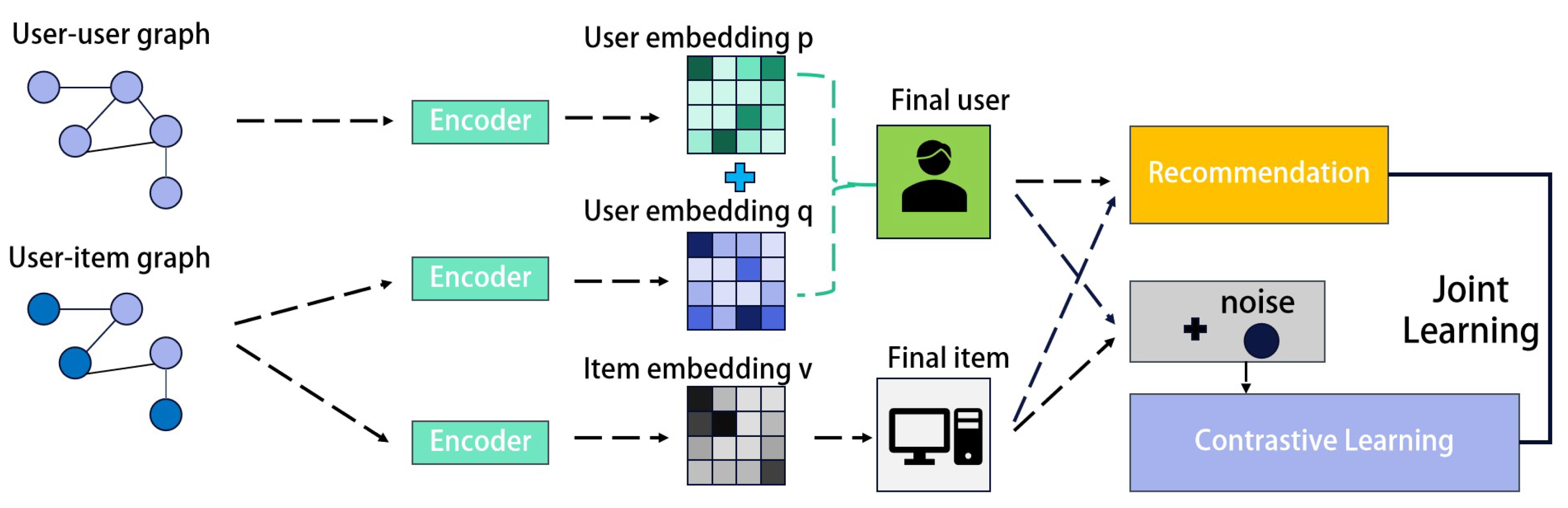
To summarize, in this paper, we propose a model called SSCGL specifically designed for social recommendation. SSCGL consists of three main modules: a diffusion module, a contrastive learning module, and a prediction module. The diffusion module learns informative user and item embedding separately from the social and interest information with a specially designed GNN-based architecture. Then, a contrastive learning module that generates contrastive views by adding noise to the graph is incorporated to further manipulate the embedding learning. Finally, the contrastive learning and the recommendation are jointly optimized to predict the final recommendation results. Experimental results on real-world social recommendation data sets validate the effectiveness of our designs.
Our work significantly contributes in the following aspects:
We successfully integrate social information and self-supervised signals into the recommendation system, significantly improving the performance.
While existing social recommendation works tend to design complex attention mechanisms to fuse the social and interest information during the GNN propagation, we abandon traditional GCN encoding and opt for a more straightforward encoder for layer-wise embedding updating. The representations from the interest and social networks are separately updated and, at last, combined with a simple sum. Our design demonstrates simple and powerful acquisition of better item and user representations.
We abandon complex graph enhancement methods commonly used in traditional contrastive learning approaches and employ a simpler and more effective approach by adding noise to embeddings, further improving the model’s performance.
We evaluate our model on three real-world publicly available data sets. Our SSGCL demonstrates superior performance, compared with eight state-of-the-art baselines, in terms of social recommendations.
3. Methodology
This section presents our proposed recommendation model, SSGCL, which consists of four components. We first introduce some essential notation. In the second and third parts, the diffusion module and prediction layer employed in our model are introduced, respectively. The training approach of the model is presented in the last part. The framework of SSGCL is illustrated in
Figure 1.
3.1. Notation
This study focuses on the social recommendation problem. Social recommendation systems generally have two sets of entities: a user set U consisting of m users and an item set V consisting of n items. Users may form two types of relationships: social connections between users and interest relationships toward items. These behaviors can be represented as a social graph and an interest graph: the social graph contains nodes denoting users and edges denoting social connections, while the interest graph contains nodes denoting both users and items, and edges denoting user preference toward the items.
These two graphs can be defined by two matrices: a user–user social relationship matrix and a user–item interest relationship matrix .
In the user–user social relationship matrix S, if user a trusts user b or, in other words, user a’s decision may be influenced by user b, ; otherwise, . We use to represent the set of all users that user a follows or trusts, i.e., .
Similarly, in the user–item interest matrix R, means user a is interested in item c, and otherwise. represents the set of items that user a is interested in, i.e., , and represents the set of users that voted for item c, i.e., .
Our goal is to find unknown preferences from users toward items; that is, a predicted new user–item matrix from R, with new preferences added.
3.2. Diffusion Module
As mentioned before, we design a diffusion module to learn comprehensive representations of users and items based on social and interest information. It has two parts, which acquire the representations from and .
First, representations are acquired from the user–item graph (interest graph
). While most GNN-based recommendation systems [
12,
31] commonly employ traditional GCN encoders to aggregate various information in the social and interest graphs, in this study, we follow [
33] and employ a simple but efficient aggregation strategy.
Specifically, both user and item representations are acquired from the interest graph. The diffusion process of the interest graph
can be defined as
Here, L is the number of stacked diffusion layers. is the representation of user i obtained from the interest graph. Similarly, is the representation of item j from the interest graph. represents the set of items j that user i is interested in, and is the set of users i that voted for item j. It is worth mentioning that the input of the first layer and are randomly initialized.
Such an encoder is better suited for GNN-based recommendation systems, as it abandons the redundant non-linear transformations of traditional GCN encoders.
The second part involves learning representations from the social graph
. Unlike the user–item graph
, the social graph only contains nodes representing users, and we can learn only user representations from it. The propagation of user
i based on the social graph
at the Lth layer could be defined as
where
is the embedding for user
i at layer
L and
is the set of socially connected neighbor users of user
i.
Upon completion of the aggregation through Equations (
1) and (
2), representations
are obtained for user
i after
L layers of iterations and
for item
j after
L layers of iterations based on the user–item graph. Through Equation (
3), the social-relation-based user representation denoted as
is obtained. To aggregate user representation learned from the social graph and the interest graph, previous works [
31] designed complex attention mechanisms and combined the two view information from every layer. However, we opt for a simple yet effective sum aggregation function to obtain the final user representation:
With our aggregation approach, both and effectively learn user representations from their respective views, making full use of the information in each graph without being subject to additional interference.
3.3. Prediction Layer
In the previous section, it is shown that the final user embedding
and the final item embedding
are obtained from Equations (
2) and (
4). Then, the prediction results of our model are calculated by taking the inner product of the final user embedding and item embedding:
where
is user
i’s predicted preference score for item
j, according to our model.
3.4. Model Training
In order to capture more collaborative signals, we employed two types of losses for joint learning to optimize the model: a supervised loss suitable for recommendation systems and a self-supervised loss to capture more collaborative signals.
3.4.1. Supervised Loss
We opted not to use point-wise loss functions [
37] which are widely used for recommendation, and instead chose the Bayesian personalized ranking (BPR) pairwise loss function instead. The BPR loss function is specialized for the ranking task. In Bayesian personalized ranking, instances with an interaction are considered positive samples, while those without interaction are considered negative samples. The objective is to maximize the margin between positive and negative samples, which is similar to contrastive learning in principle. This matches our need to determine which items are more worthy of recommendation to the users (potential positive samples with high ranking). Additionally, recommendation data are sparse, with positive samples (instances where users interact with items) being far fewer than negative samples. The sampling-based BPR loss can satisfactorily resolve this problem and lead to better performance. The BPR loss is defined as
where
is the training data,
represents the observed interaction information, and
denotes unobserved interactions.
is the sigmoid function. The BPR loss provides positive and negative signals to model the user–item interaction but still lacks the ability to enhance the embedding based on the nodes themselves. This could potentially result in sub-optimal representations. To address this issue, we employed a specially designed contrastive loss as assistance.
3.4.2. Self-Supervised Loss
To create contrastive views, traditional GNN-based contrastive learning involves pre-processing steps, such as randomly dropping nodes or edges, performing random walks, or even constructing an entirely new graph [
23]. Such strategies tend to be over-designed. According to the findings of previous work, steps such as randomly dropping nodes and edges are likely to result in the loss of important information [
36]. Moreover, enhancing the graph in these ways can be very time-consuming.
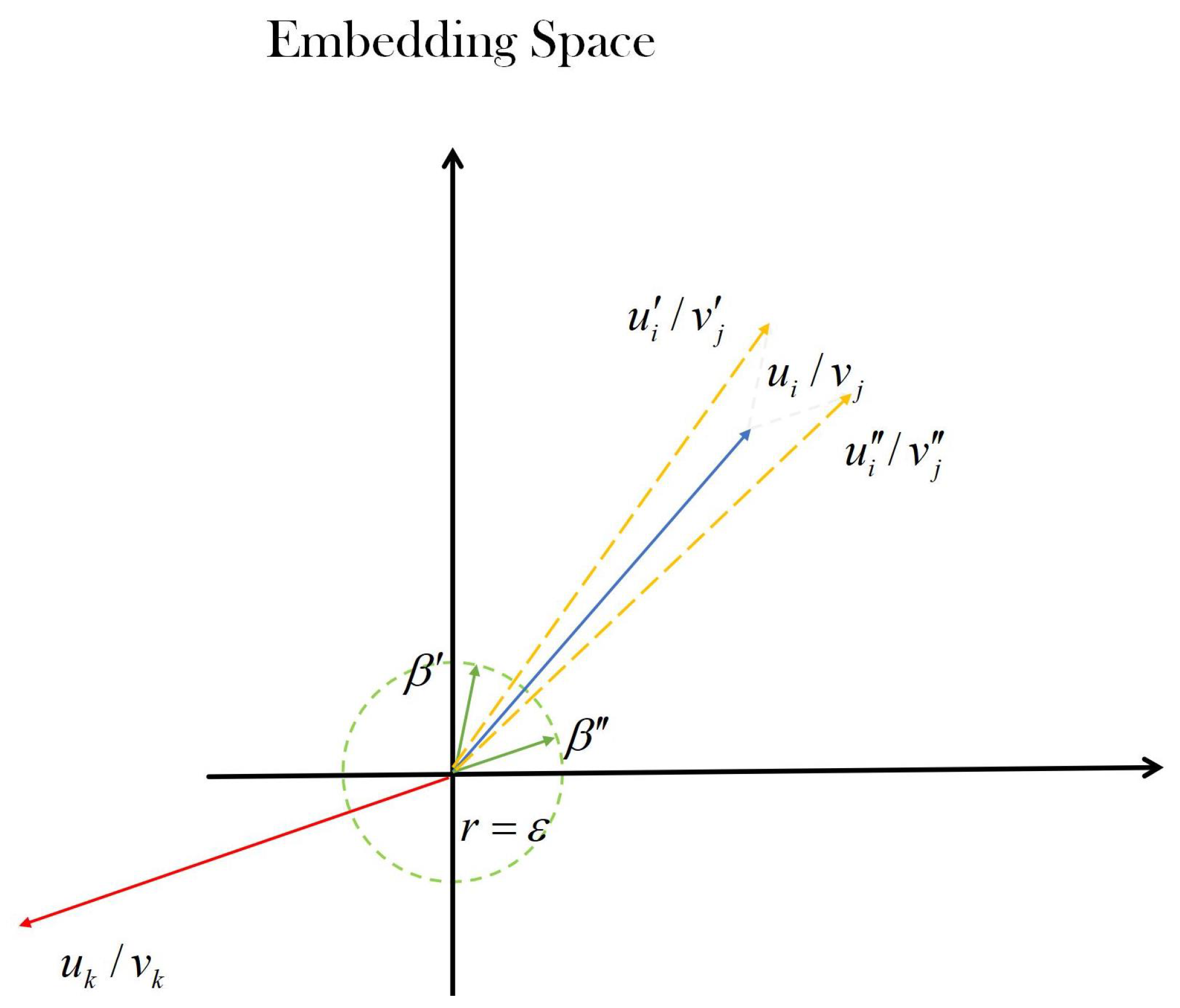
Therefore, here, we adopt a simpler and more efficient contrastive learning approach. Inspired by [
36], traditional graph enhancement methods are abandoned and instead positive and negative samples are constructed by adding noise to the learned embedding of users and items. In particular, for a user embedding
, samples
and
are generated as follows:
Here, for user
i with learned representation
,
and
represent the added vector noises. These noises are constrained by
and
,
.
is a hyperparameter and ⊙ is the Hadamard product. These constraints control the magnitude and the orthant of the noise, which could otherwise lead to significant biases and disrupt the original semantics of the node.
Figure 2 briefly illustrates our contrastive learning method described in Equation (
7).
We consider samples generated from the same node as positive pairs and samples from different nodes as negative ones for contrastive learning. This simple strategy can smoothly manipulate the learned representation toward a better distribution. The InfoNCE contrastive loss [
38] is employed to force positive pairs close to each other and negative pairs distant from each other,
Here, denotes the cosine similarity between two vectors. is a temperature hyperparameter. The denominator is summed over all possible users k in the user set U. This contrastive loss can be regarded as a softmax classifier that classifies to .
Similarly, for item embedding
, the following is the item-based noised samples and contrastive loss:
The final self-supervised loss is the sum of the user-based contrastive loss and the item-based contrastive loss:
3.4.3. Final Loss
We incorporated our supervised BPR loss (refer to Equation (
6)) with our self-supervised contrastive loss (refer to Equation (
11)) for joint learning and to optimize our model. The final loss function is defined as
where
is the regularization term of
introduced to prevent model overfitting.
and
are two hyperparameters used to control the balance. The learning process is conducted in a supervised manner. The BPR loss is the primary supervised component that optimizes the user and item embedding, while the self-supervised learning module merely serves as an auxiliary part that manipulates the learned embedding toward a better distribution.
4. Experiments
In this section, to demonstrate the effectiveness and superiority of our model, we conducted extensive experiments and addressed the following questions from various perspectives:
- -
RQ1: How does our model perform compared with various state-of-the-art (SOTA) models on different data sets?
- -
RQ2: How do the self-supervised learning module and diffusion modules’ propagation mechanisms impact the model?
- -
RQ3: How do different parameter settings affect the model?
4.1. Benchmark Data Sets
We utilized three real-world publicly available data sets: Yelp [
23], Last.fm [
39], and Douban-book [
36]. Below, detailed information about the data sets is provided.
Yelp: Yelp is a geographically based online review platform that encourages users to share their perspectives and experiences by writing reviews and providing ratings. The data set encompasses interactions between users and various locations, including visits and comments. Additionally, by leveraging user friend lists, we can infer user relationships, enabling further analysis of influencing factors within the social network.
Douban-book: Douban-book is a highly influential book-related online social platform in China that gathers extensive information on books and user reviews. This platform enables users to search for books, share their book reviews, rate works, and create personal booklists. Additionally, users can follow other readers, thereby establishing a social network to receive more book recommendations and enhance their interactive experiences.
Last.fm: Last.fm is a music-related data set that includes user, artist, song, and social relationship data. It is widely used in research on music recommendation systems, social network analysis, and music data mining. The data set comprises information such as users’ listening histories, social relationships, tags, and events, providing valuable resources for studying music consumption behavior and music social networks.
The three data sets are publicly available for download. All processed data sets were obtained from
https://recbole.io/cn/dataset_list.html (accessed on 6 March 2024). A summary of the data set details is provided in
Table 1. The data sets were all pre-processed [
40] and have been widely used for the recommendation task. Our focus was solely on the social interest information within the data sets, while other user attributes and item details were not within the scope of our consideration.
4.2. Baseline Methods
In the experiments, we compared a total of eight recommendation system models with our proposed SSGCL. The main differences between these baselines are summarized in
Table 2.
MF-BPR [
28] is a recommendation system model. Built upon the idea of matrix factorization, it aims to learn latent representations of users and items for personalized item recommendations. The model is optimized using Bayesian personalized ranking (BPR) loss.
Social-MF [
26] is a model designed for recommendation systems. It is also based on the idea of matrix factorization, integrating social information with purchase data to provide personalized recommendations.
NGCF [
30] is a deep learning model for recommendation systems, combining traditional collaborative filtering methods with graph neural networks to enhance the effectiveness of personalized recommendations. The core idea involves representing users and items as nodes in a graph and using graph neural networks to learn their latent relationships. Through multiple layers of neural networks, NGCF can better capture the complex interactions between users and items, thereby improving the model performance.
Diffnet++ [
31] is a graph diffusion model for social recommendations. It combines social and interest information in a recursive manner and employs an attention mechanism during the propagation and aggregation process to enhance the model’s performance.
MHCN [
41] is a model based on hyper-graph convolutional networks for recommendation systems. The model utilizes social and other information to model edges in the hyper-graph, thereby enhancing the recommendation performance of the model.
LightGCN [
33] is a lightweight graph convolutional model. In comparison with traditional graph convolutional networks (GCNs), it simplifies the structure and parameters. By directly updating user and item embedding vectors, it enhances the learning efficiency and effectiveness in social networks and recommendation systems.
SGL [
23] is a graph convolutional model that incorporates self-supervised learning for recommendation systems. The algorithm enhances the graph to transform the original graph and create different views by using uniform node and edge dropout strategies. Subsequently, it employs contrastive learning methods to learn from these views. The losses are jointly optimized to obtain the final representations of nodes.
SEPT [
42] is a recommendation system model that incorporates self-supervised learning. By constructing complementary views of the graph, pseudo-labels are obtained, and triplet training is employed to assist the training process.
4.3. Experimental Setup
For the effectiveness and fairness of the experiments, we adjusted the hyperparameters for all baselines following the strategies in the original papers. We ran all experiments with the Adam optimizer. The data sets were randomly divided into training, validation, and test sets in an 8:1:1 ratio. Meanwhile, we employed two advanced and effective evaluation metrics that are widely used in top conferences [
31,
33,
36,
43]—namely Recall@K and NDCG@K (normalized discounted cumulative gain)—to assess the model performance. In our SSGCL model, we stacked three GNN layers for the influence diffusion, and the embedding size for both users and items was set to 64. The L2 norm was employed for the regularization. The trade-off hyperparameters of the contrastive learning module
and the regularization term
were set to
and
, respectively. The learning rate
was set to
. The temperature coefficient
was
. The noise radius
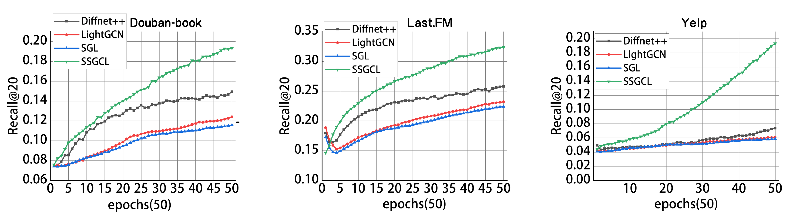
is 0.1. Additionally, all our experiments were conducted on an RTX 2070 (8 GB) GPU, and the results of the first 50 epochs are illustrated in
Figure 3.
4.4. Performance Comparison (RQ1)
This study compared eight baseline models with two variants of SSGCL, namely SSGCL-M and SSGCL-L, across three public data sets and two evaluation metrics. SSGCL-M was the model that only aggregated the user representation of the two graphs in the last GNN layer, as described in our Methodology section. SSGCL-L was a variant of our model in which we followed previous works and aggregated the user representation at each layer of the GNN influence diffusion. The learned user representation that combined two sides of information was then updated into the two graphs for the influence diffusion of the next GNN layer.
We conducted the experiment by evaluating the rankings for the top 10, top 20, and top 30 recommendations. As shown in
Table 3,
Table 4 and
Table 5, our SSGCL-M (final aggregation) consistently outperformed the optimal baseline in the top@k experiments, while SSGCL-L (intermediate aggregation) achieved a performance close to the baseline. We summarize our findings as follows:
- 1.
The exploration of social information could benefit the recommendation system.
The tables show that many recommendation systems that incorporate social information performed better than other methods proposed during the same time period, such as Diffnet++, SEPT, and our method. However, the advantages of social information were not apparent when compared with more up-to-date methods. This was probably because taking full advantage of social information is difficult. Early approaches lack effective ways to jointly learn social interactions with the interest information.
- 2.
The approaches based on GNNs exhibited excellent performance.
From the tables, it is evident that GNN-based models generally exhibited a significant improvement over traditional approaches, such as matrix factorization-based recommendation systems. For example, LightGCN and SGL performed quite well without social information, and mainly benefited from their well-designed GNN layers. MHCN involves both social information and self-supervised signals but has yet to achieve satisfactory results, which may be because it fails to model multifaceted information sufficiently without the assistance of GNNs. This demonstrates a GNN’s effectiveness in handling such interest and social networks, as well as modeling the complex interactions in the recommendation task.
- 3.
Self-supervised learning shows great potential in recommendation system tasks.
It can be observed from the tables that recent recommendation system approaches, such as SGL and SEPT, tended to employ self-supervised learning and obtained satisfactory performance. This was because the self-supervised learning module could help to learn more informative representations and make the user and item representation uniform, thereby helping to achieve better recommendation results.
- 4.
The superiority of our SSGCL.
Our SSGCL sufficiently explored the social and interest network with a GNN-based influence diffusion layer. The learned representation was further optimized with a contrastive learning module that extracts self-supervised signals. This should be the reason why our SSGCL performed well compared with the baseline methods.
4.5. Ablation Study (RQ2)
Ablation experiments helped us gain a deeper understanding of the contributions of different components of the model to the overall performance. Through gradually removing specific parts of the model or altering their configurations, we assessed the impacts of these parts on the model’s performance, thus revealing key factors in the model design.
From the above experiments, we could observe that both SSGCL-L and SSGCL-M performed well. The variant SSGCL-L adopts a more complicated influence diffusion strategy that aggregates the user representation at each layer like in many other algorithms that take social information into account. However, it cannot beat SSGCL-M, which has a simple final aggregation strategy.
In this subsection, to further investigate the effectiveness of the model’s simple influence diffusion strategy and the contrastive learning module, we conducted ablation experiments to address the question of whether simpler aggregation mechanisms and contrastive learning make sense. For this purpose, we compared four variants of the model, namely SSGCL-M utilizing final layer aggregation with contrastive learning, SSGCL-L employing intermediate layer aggregation with contrastive learning, SSGCL-N using final layer aggregation without contrastive learning, and SSGCL-O using intermediate layer aggregation without contrastive learning. To ensure the fairness of the ablation experiments, we used the same optimizer and other parameters as mentioned before.
From
Table 6,
Table 7 and
Table 8, it is evident that SSGCL-M achieved the best performance on all three public data sets. This further shows the effectiveness of our simple final layer aggregation and the contrastive learning module. SSGCL-M performed better than SSGCL-L, and SSGCL-N performed better than SSGCL-O, both of which demonstrated that the precisely designed propagation of previous social recommendation systems did not have much of an effect on the final performance; furthermore, our final aggregation strategy was simple and effective, and it lead to better representations and recommendation results. SSGCL-M and SSGCL-L clearly outperformed the other two variants, which shows the superiority of our contrastive learning module.
4.6. Hyperparameter Analysis (RQ3)
In this subsection, we present the results of the experiments that were conducted to explore the sensitivity of several key hyperparameters in our model. Analyzing the parameter sensitivity helped us to better understand the behavior and performance of the model. Through experimenting with and evaluating different parameter values, we can understand how the model’s performance changed under different settings, thereby determining the optimal parameter combination.
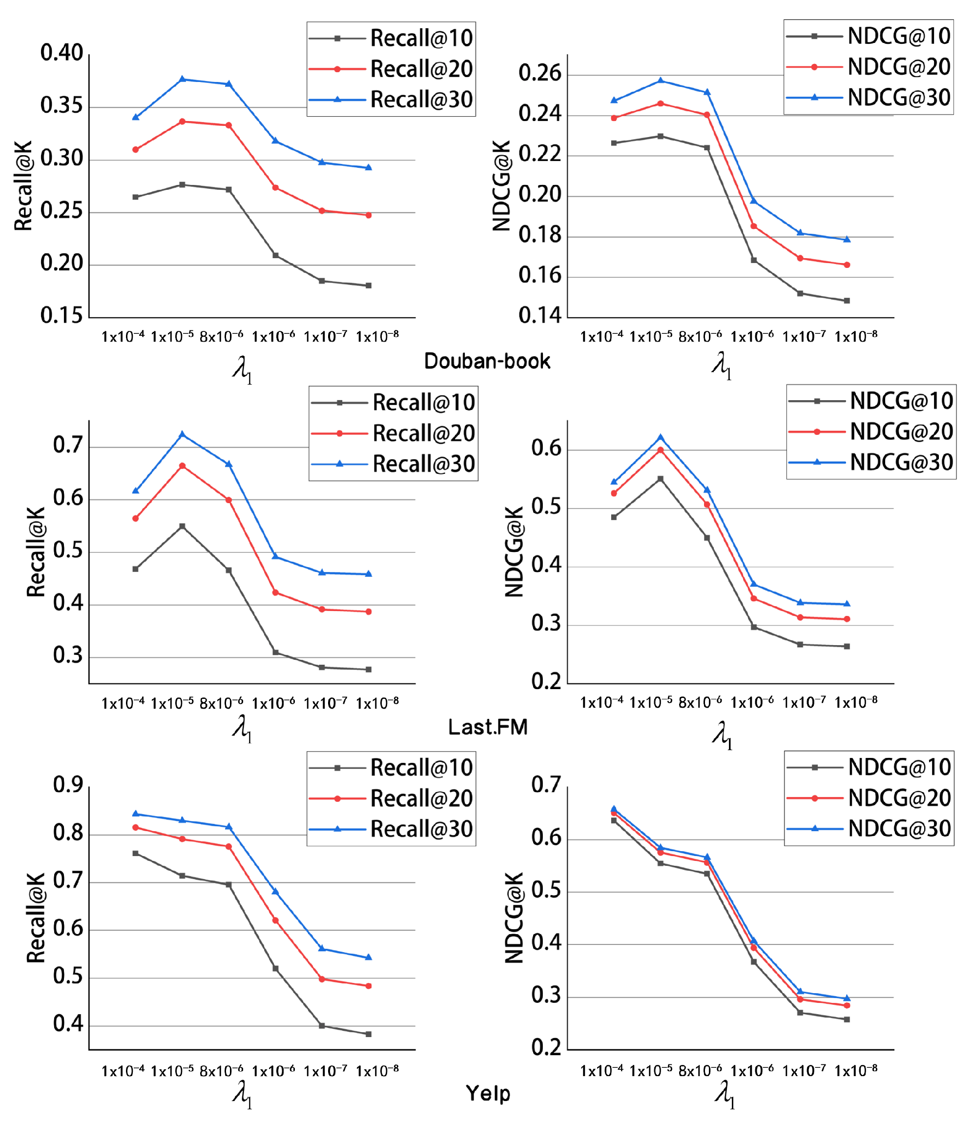
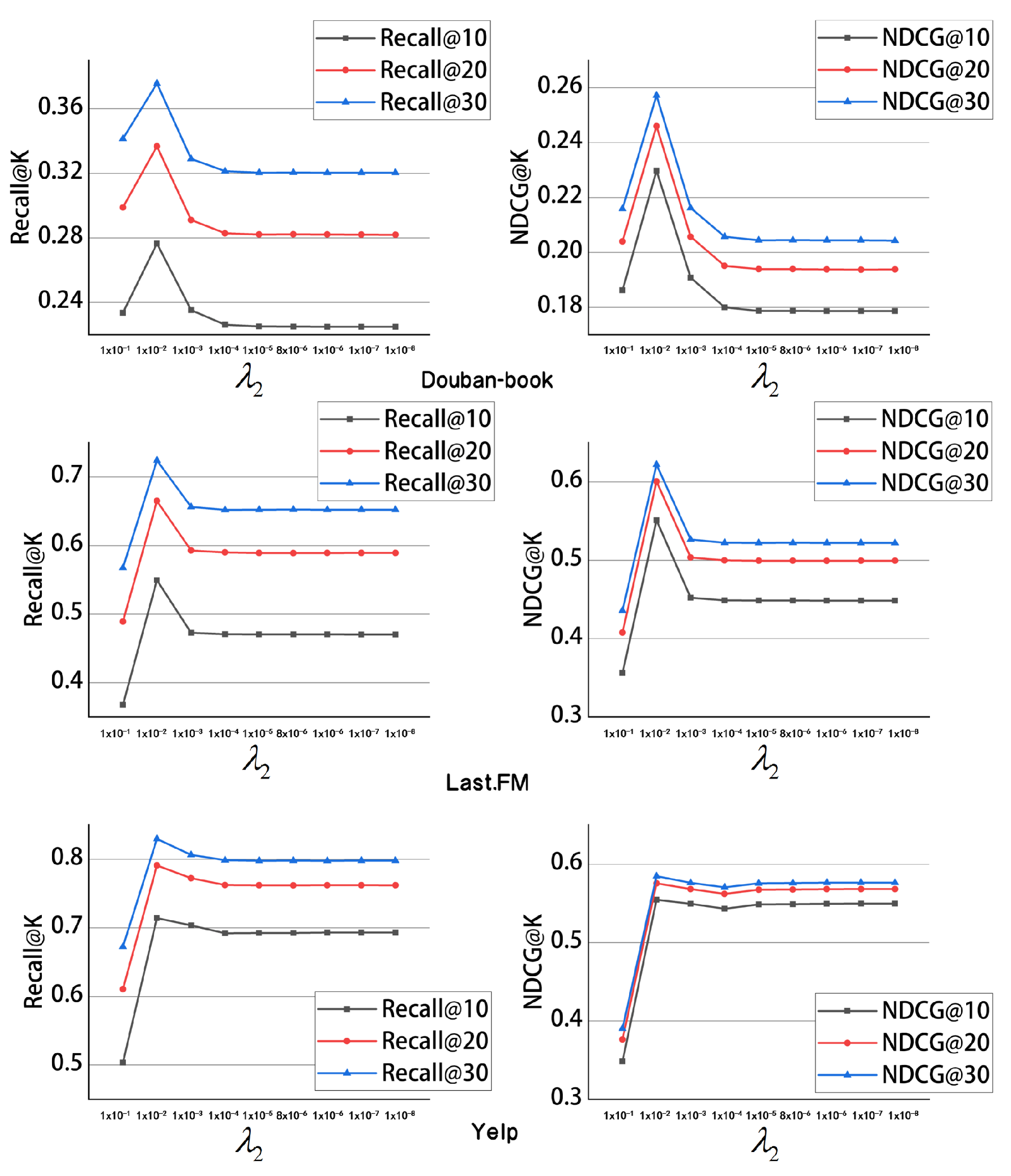
The contrastive learning coefficient : We conducted experiments on the contrastive learning coefficient
, and the results are shown in
Figure 4. The model performance peaked on the Last.fm and Douban-book data sets when the contrastive learning coefficient reached
. For the Yelp data set, when the contrastive learning coefficient reached
, the model performance peaked. This shows that adjusting the parameters on different data sets can optimize model performance, as different data sets exhibit varying sensitivities to parameters.
The regularization coefficient : We conducted experiments on the regularization coefficient
. The main purpose of the regularization parameter
is to control the complexity of the model, thereby helping to prevent overfitting. When the model becomes overly complex, it may perform well on the training data but poorly on unseen data, indicating a lack of generalization to new samples. By introducing the regularization parameter, a penalty term was added to the loss function, penalizing the size of the model parameters, which made the model simpler and improved its generalization capability. The results are shown in
Figure 5. We observed that when the regularization parameter was set to
, our model achieved the best performance on all data sets, which was different from the case of the contrastive learning coefficient. Additionally, we found that when we set the parameter between
and
, the experimental results on the Douban-book and Last.fm data sets remained stable, with the graph lines leveling off. This trend was more rapid on the Yelp data set. When the parameter was set in the range of [
,
], the experimental results stabilized, and the decrease in model performance was minimal. These findings provide guidance for selecting and adjusting regularization parameters, emphasizing the importance of finding optimal parameters within a certain range to achieve stable and excellent model performance.
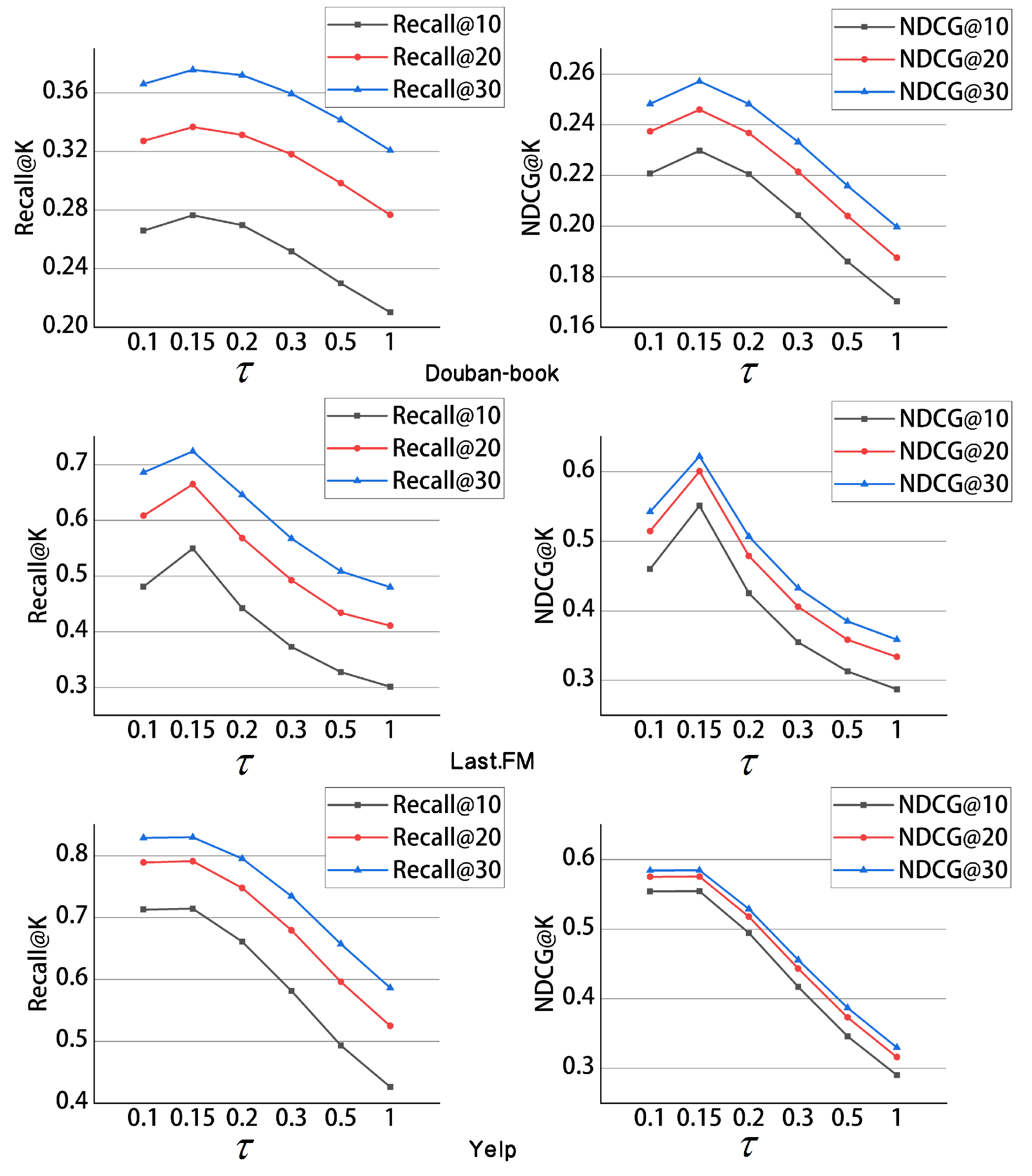
The temperature coefficient of InfoNCE : The temperature coefficient
plays a crucial role in adjusting the scale of the contrastive size. The main function of temperature coefficient
is to control the proportion of positive and negative sample pairs. From a mathematical perspective, the temperature coefficient
in Equation (
8) is positioned in the denominator.
Figure 6 clearly shows that, when the model parameter was set to 0.15, the best performance was achieved on all three data sets. On the Douban-book and Last.fm data sets, the model performance showed an upward trend as the value of parameter
increased within the range [0.1, 0.15]. However, when the parameter was set to [0.15, 1], the model performance started to decline. On the Yelp data set, the model performance remained relatively stable within the range [0.1, 0.15], but exhibited a declining trend within the range of [0.15, 1]. Overall, the optimal performance was achieved when the model parameter was set to 0.15.
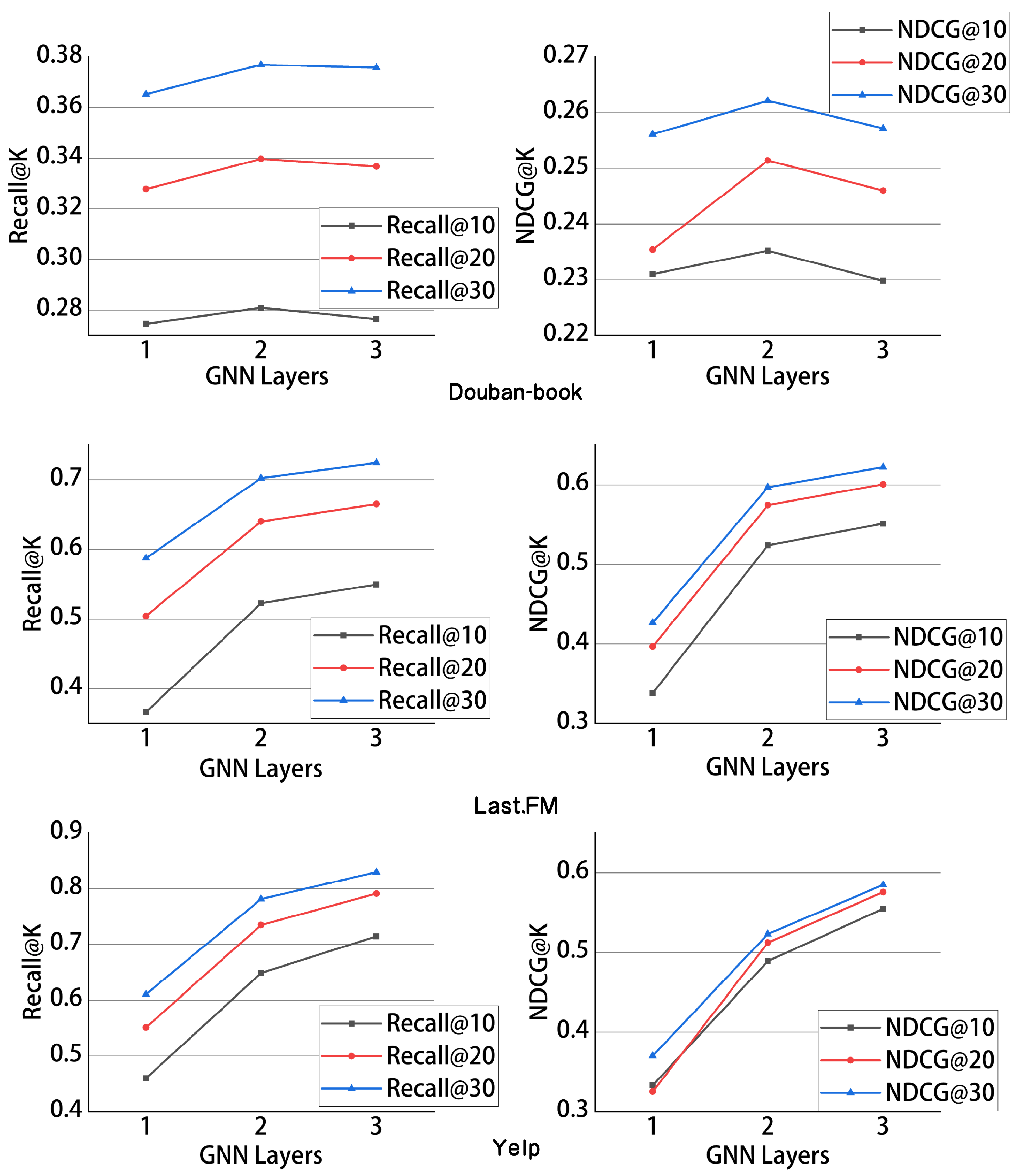
Number of GNN layers: Due to the excessive smoothing issue of GNNs, we conducted experiments to explore the best number of GNN layers for our model. The experimental results are shown in
Figure 7. For the Last.fm and Yelp data sets, as the number of GNN layers increased, the model’s performance improved, reaching its peak when the number of GNN layers was set to three. However, on the Douban-book data set, the model performance peaked when the GNN layers reached two. This indicates that different data sets exhibited varying sensitivities to the number of GNN layers. The Douban-book data set, being larger and more intricate in its interrelations compared with the other two data sets, further underscored the issue of excessive smoothing in graph neural networks (GNNs). When data sets exhibit denser and more diverse interaction patterns, increasing the number of GNN layers may lead to over-smoothing of the features, resulting in a loss of detail and discriminative power in the learned features.
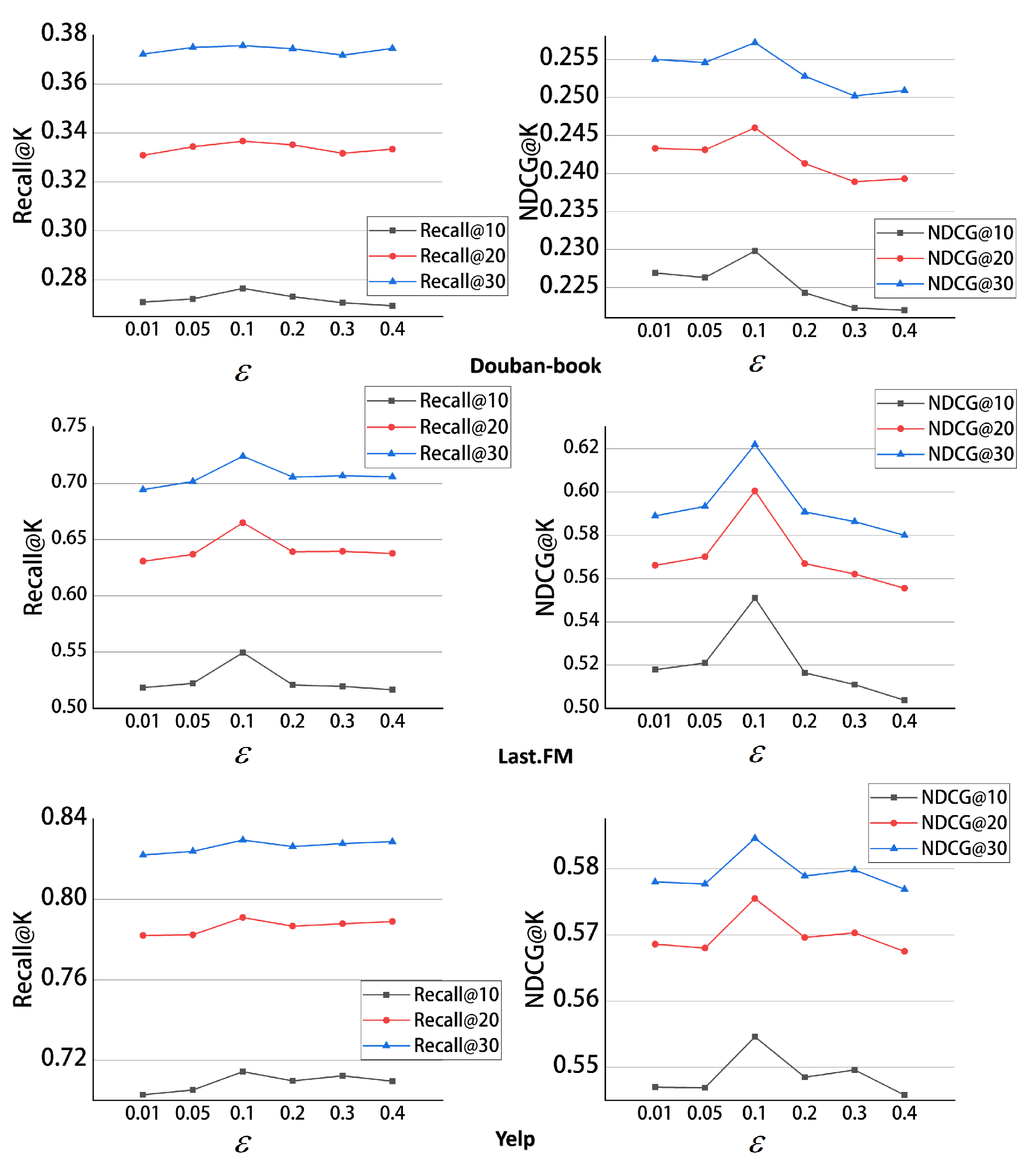
Noise radius : We abandoned traditional graph augmentation methods, such as random node deletion or random edge deletion, opting instead to introduce uniform noise into the samples to construct sample pairs and simultaneously enhance the model’s robustness. However, the introduction of noise must be constrained, as excessive noise can severely impact the model. Therefore, we imposed a radius constraint on the noise introduced to ensure the effectiveness and stability of the model. We conducted experiments with the noise radius parameter
set to 0.01, 0.05, 0.1, 0.2, 0.3, and 0.4. We found that the model achieved optimal performance across all three data sets when the noise radius r was set to 0.1. Moreover, as the noise radius
increased, the decreasing trend in performance tended to stabilize. This indicates that our model has a certain level of robustness. The experimental results are shown in
Figure 8.
Through the parameter sensitivity experiments, we found that the data distribution varied across each data set, leading to the requirement of different parameter configurations for the model to achieve optimal performance. Therefore, we had to adjust the parameters to obtain the best performance. This also implies that in recommendation systems, we can enhance the generalization performance by adjusting the parameters. In other words, parameter adjustment can improve both the applicability and performance of the recommendation system.
5. Conclusions and Future Work
This paper proposes a simpler and more effective social recommendation system called SSGCL. Specifically, we explore simpler aggregation methods and design a GNN-based influence diffusion module that learns informative user and item representations from both the interest network and the social network. A special contrastive learning module is then employed, which generates positive and negative samples by simply adding noises to the original node embedding to manipulate the learned representations for a better distribution. The experiments demonstrate that some of the strategies in previous social recommendation models are over-designed, while our model is effective and simple. We achieve state-of-the-art results on three public data sets in terms of two evaluation metrics.
While our recommendation model has made significant progress in terms of performance, there are other issues and limitations inherent in recommendation systems that should be recognized. For instance, most existing recommendation systems face the risk of data leakage because they utilize users’ private data and do not consider privacy protection, making these data vulnerable to malicious attacks. Some companies choose to completely safeguard data or withhold labels during training to prevent data leakage. However, while this approach ensures data security, it sacrifices data interactivity, leading to sub-optimal model performance during training. Similar issues are addressed in other scenarios but not well explored for recommendation systems yet. Furthermore, social influence and algorithmic bias are also common issues in recommendation systems. Recommendation systems may excessively filter user information, causing users to only encounter information related to their interests, neglecting other important information and leading to societal fragmentation. Ensuring more diverse recommendations while improving recommendation system performance remains a challenge and a focal point for future efforts.
Although these issues are outside the scope of this paper’s consideration, we intend to address them in our future work. In our future research, we aim to broaden our focus to explore the robustness of recommendation systems and their security and privacy concerns to better align with real-world applications and offer numerous intriguing avenues for future exploration. Additionally, we would also like to introduce more information, whereas this study focused solely on social recommendation systems, primarily incorporating social information. For example, there has been a surge of interest in knowledge graphs [
44] within the field of recommendation systems. In this way, we can potentially uncover more latent relationships and achieve superior performance.
Regarding future work, as mentioned, there has been a surge of interest in knowledge graphs [
44] within the field of recommendation systems. Knowledge graphs offer the capability to integrate various types of data, whereas this study focused solely on social recommendation systems, primarily incorporating social information. Introducing knowledge graphs into recommendation systems could potentially enrich the system with a broader range of information, thereby uncovering more latent relationships and achieving superior performance. On the other hand, incorporating additional information into recommendation systems may pose challenges, such as compromising model robustness and introducing excessive noise [
19]. In our future research endeavors, we aim to broaden our focus beyond solely self-supervised learning of graphs. Instead, we intend to explore a wider array of topics, including the semi-supervised learning of graphs [
45], the security of graph data [
46], and privacy concerns in graph recommendation systems [
47]. This expansion will enable our recommendation systems to better align with real-world applications and offer numerous intriguing avenues for future exploration.


