1. Introduction
In the fields of science and engineering, optimization problems, especially those with constraints, play a crucial role. Constrained optimization problems (COPs) are vital in a wide range of applications, including process control [
1,
2], reactor design [
3], and production scheduling [
4]. Among these, specific challenges such as tension/compression coil spring design [
5] highlight the intricate nature of these problems. The aim of addressing COPs is to enhance design efficiency, minimize experimental costs, and reduce testing cycles. These problems hold intrinsic value across various engineering disciplines, including chemical, mechanical, and electrical engineering [
6,
7,
8], as they seek optimal solutions within the boundaries set by constraints, be they equalities or inequalities [
9]. To solve these complex issues, a range of methodologies have been developed, from gradient-based methods [
10], known for their efficiency in differentiable problems, to population-based strategies like Genetic Algorithms [
11], which are capable of addressing non-differentiable and multi-modal challenges, albeit often at a higher computational cost [
12]. COPs are typically represented through mathematical formulations, underscoring their quantitative nature and the systematic approach required for their resolution. We define the formulation
where
is a solution vector within the solution space
,
represents the constraints, and
and
are the lower and upper bounds of the constraints, respectively. There are two types of scenarios for the solution to this formulation: feasible and infeasible. A solution is considered feasible if the solution vector
satisfies all the constraints
. Conversely, a solution is deemed infeasible if
but does not satisfy all the constraints
. At times, the feasibility ratio (the percentage of feasible solutions out of the total number of feasible and infeasible solutions) can be very low, which is equivalent to having very stringent constraints. In such cases, it is imperative to find a solution that satisfies the constraints as efficiently as possible.
For solving complex optimization problems, especially those with constraints, the use of surrogate models has emerged as a highly effective strategy. Surrogate models, pivotal in the realm of optimization, provide simplified yet powerful approximations of complex systems, enabling efficient exploration and optimization of design spaces where direct evaluations are prohibitively expensive. These models, also referred to as metamodels, span a diverse array of methodologies, each tailored to capture the intricacies of different problem domains [
13]. To encapsulate these varying surrogate model methodologies and their application in constrained optimization problems,
Table 1 provides a comprehensive summary of the key literature, highlighting techniques, tested datasets, and their respective advantages and disadvantages.
Despite these advancements, a comprehensive review of the literature underscores certain limitations in the current surrogate modelling approaches, particularly when applied to constrained optimization problems [
18]. A notable challenge is the difficulty in accurately capturing and adapting to the complex constraint boundaries that often define feasible regions in optimization landscapes [
19]. Many existing surrogate models excel in unconstrained scenarios or situations with simple constraints but may fall short when faced with complex, nonlinear, or high-dimensional constraints [
20]. Additionally, there is a paucity of methodologies that effectively incorporate constraint handling mechanisms within the surrogate model itself, often relying on external penalty functions or constraint relaxation techniques that may not always yield optimal solutions. This gap in the literature highlights the need for more sophisticated surrogate models that can inherently deal with complex constraints while maintaining the balance between exploration and exploitation in the search space. These insights into the limitations of current surrogate models in handling constrained optimization problems have motivated the development of our proposed methodologies. By addressing these identified gaps, we aim to contribute to the advancement of surrogate-assisted optimization strategies, providing more robust and efficient solutions for complex constrained optimization challenges.
Among the diverse array of surrogate modelling techniques, Gaussian Process Regression (GPR) stands out for its efficiency and effectiveness [
17]. GPR is renowned for its robustness in capturing the underlying trends of the data with a quantifiable measure of uncertainty, making it particularly suitable for optimization problems where uncertainty plays a critical role [
21]. The historical development of surrogate models in optimization was notably advanced in 1998 when Jones et al. [
22] introduced the Efficient Global Optimization (EGO) algorithm. This algorithm integrates GPR with the Expected Improvement (EI) function, a pivotal concept in Bayesian optimization. The EI function is designed to systematically identify the global optimum of computationally expensive black-box functions, which are often subject to inherent uncertainties [
23]. This approach prioritizes sampling in regions where the anticipated improvement in the function’s value is maximized, thereby enhancing the model’s accuracy in critical areas. This methodology exemplifies an active learning strategy, dynamically refining the model with each new data point to efficiently navigate the complex landscape of the optimization problem. However, when dealing with optimization problems that include stringent constraints, the standard EI approach may require modifications to accommodate these limitations. In response to this challenge, recent developments have introduced variants such as the Constrained Expected Improvement (CEI), which adapt the EI principle to handle constraints effectively [
24,
25].
In addressing the challenges inherent in constrained optimization, this study introduces significant innovations that extend the current state-of-the-art methodologies. Firstly, we propose a novel approach to compute the Expected Prediction Error (EPE) [
26] at an untested point by leveraging the cross-validation error from a nearby tested point. This method enhances the prediction accuracy of our surrogate model, particularly in the sparse regions of the design space where traditional interpolation methods might falter. Secondly, we introduce the Constrained Expected Prediction Error (CEPE) criterion, a pioneering metric designed to navigate the intricate landscape of constrained optimization problems efficiently. By integrating CEPE within a Differential Evolution (DE) [
27] framework augmented with Gaussian Process (GP) surrogates, our approach not only capitalizes on the strengths of evolutionary algorithms in exploring complex solution spaces but also harnesses the predictive prowess of GP models to make informed decisions during the optimization process. The synergy between these innovations presents a robust framework that promises improved optimization performance, especially in scenarios characterized by stringent constraints and expensive function evaluations.
The remainder of this paper is structured as follows. In
Section 2, we introduce the theoretical knowledge about Gaussian Process, Expected Improvement and Expected Prediction Error. In
Section 3, we discuss methodologies for Constrained Expected Improvement, introduce our novel method Constrained Expected Prediction Error, and provide the GP surrogate-assisted Differential Evolution (DE) algorithm. In
Section 4, we evaluate the efficacy of CEI and CEPE using benchmark problems, and in
Section 5, we illustrate their application in a real-world problem. Finally, we conclude this paper with discussions and remarks in
Section 6.
2. Background and Concepts
In this section, we provide a brief theoretical overview of Gaussian Process Regression (GPR), Expected Improvement (EI), and Expected Prediction Error (EPE).
2.1. Gaussian Process Regression
We aim to use the Gaussian Process Regression (GPR) framework to model an unknown function
, by assuming that
is a sample from a Gaussian process denoted as
. Within this context, for any input point
, the function value
is viewed as a sample from a Gaussian random variable
and
is distributed as
, where
and
are constants independent of
. The covariance of
with another random variable
, where
represents another point in the input space, is given by
The correlation function
is defined as
where
p is the dimension of the input space and
are the hyperparameters.
Considering a set of
N input points
, let
and
. The parameters
can be estimated by maximizing the joint Gaussian probability density function of
at
where
is an
matrix with elements
, and
is an
N-dimensional column vector of ones.
The log-likelihood function is then
Now, let us differentiate the log-likelihood with respect to
:
Setting this derivative to zero and solving for
gives the maximum likelihood estimate
Next, let us differentiate the log-likelihood with respect to
Setting this derivative to zero and solving for
gives the maximum likelihood estimate
There is no analytical form for the estimates of , so the maximization of the log-likelihood function with respect to is usually completed by conjugate descent.
With the maximum likelihood estimates of the parameters, we can now derive expressions for predicting
at a new point
. Let
be the vector of correlations between the new point and the
N data points, where the
i-th element of
is
. The best linear unbiased predictor (BLUP) of
can be written as:
where
is the estimate of the mean in (
7) and
is the correlation matrix calculated using the estimates of
.
Similarly, the prediction variance can be derived as:
This forms the basis for Gaussian Process Regression, where we model the unknown function as a Gaussian process and make predictions at new points by combining information from the observed data.
2.2. Expected Improvement
In this section, we introduce a widely-adopted infill sampling method known as Expected Improvement (EI), developed by Jones et al. [
22] for the optimization of expensive black-box functions. Expected Improvement is particularly useful once a surrogate model, typically Gaussian Process Regression, is constructed.
As previously defined in Equation (
1), let
denote the objective function with a surrogate model
that follows a Gaussian process. Consider a set of test inputs
with corresponding observed function values
. We define
as the best observed value of the function among the test inputs, i.e.,
. The improvement of
at a new input point
is defined as
Expected Improvement is then defined as the expected value of this improvement, given the observed data
Through some non-trivial mathematical manipulations, we can express the Expected Improvement in terms of the predictive mean and standard deviation of the surrogate model as follows:
where
and
are the predictive mean and standard deviation of the surrogate model at
, computed according to Equations (
10) and (
11), and
and
denote the probability density function (PDF) and cumulative distribution function (CDF) of the standard normal distribution, respectively.
2.3. Expected Prediction Error
In this section, we introduce the Expected Prediction Error (EPE), an active learning strategy employed to evaluate the accuracy of a predictive model. EPE quantifies the discrepancy between the predicted and actual values. Specifically, it is the expected value of the squared prediction error over a sample of data. EPE is sometimes referred to as the mean squared error (MSE).
Within the context of the GPR methodology, the posterior distribution of the response at a given location
is denoted as
, which follows a Gaussian distribution expressed as
. In this setting, the mean
symbolizes the predictive estimate given by
, while the variance
reflects the uncertainty associated with the prediction, denoted as
. Given this framework, we can define the prediction error, often referred to as the loss function,
, for a point
as
Here, embodies the true underlying response, perturbed by inherent observational noise.
Then, the overall generalization error of the GPR-based surrogate model is given by
where
denotes the expected value of the prediction error, and
is a subset of
. This expectation can be decomposed into
where the first term represents the squared bias, capturing the average difference between the predicted and observed responses; the second term is the prediction variance of the surrogate model; and the third term is the variance of the noise
, which is often negligible.
The EPE quantifies the discrepancy between the GPR model’s predictions and the true function values. In this context,
denotes the true function we aim to approximate, and
represents the GPR model’s prediction at
. Thus, EPE at a point
is given by
However, the true response
is unknown in the bias term. Following the approach by Liu et al. [
26], we employ leave-one-out cross-validation for estimation. Initially, we estimate the cross-validation errors at all training sample locations:
where
represents the
i-th training sample, and
denotes the GP model trained using all training samples except
. Next, for any point
, we locate the nearest training sample to
, denoted as
, and assign its associated cross-validation error to
:
Finally, incorporating the cross-validation error, we obtain a refined expression for the EPE:
The Expected Prediction Error (EPE) plays a crucial role in assessing the accuracy and reliability of our surrogate model, particularly in constrained optimization problems. By calculating the EPE, we can identify regions in the design space where the model’s predictions are less reliable, informing us where additional sampling might be beneficial. Moreover, as EPE comprises both bias and variance, it aids in striking a balance between the two, ensuring that the model is neither too simplistic nor too complex. This information is vital for efficient exploration of the search space and making informed decisions in the optimization process.
3. Methodology
In this section, we first present the CEI method proposed by Jiao et al. [
25], then we introduce a novel method CEPE for solving constrained optimization problems (COP). To solve a COP, the objective is to minimize the objective function subject to several constraints. Before delving into the details of our proposed method, we will define some notations in the following subsection.
In this work, we treat
as an untested point, while
are considered tested points. Let
denote the objective function, and
represent the constraint functions for
. For a given point
, we define a Gaussian random vector
as
We introduce as a Gaussian random vector to represent the constraints’ evaluations at the point . This probabilistic modelling approach allows us to account for and manage the uncertainties associated with constraint evaluations, especially when exact determinations of these constraints are not feasible or when they are subject to variability due to measurement errors, model inaccuracies, or other sources of uncertainty.
For a set of
N tested points
, we define the following Gaussian random vectors:
where
,
,
, …,
, and
represent the function values at the tested points. In contrast,
and
are the quantities to be predicted. The evaluated function values are
which are considered as samples of
,
,
, …,
, and
. Essentially, by using the known function values, we can predict
and
for
at the tested points
without additional function evaluations.
3.1. Constrained Expected Improvement
In the exploration of constrained optimization problems, we often encounter a combination of both feasible and infeasible solutions, as categorized by Jiao et al. [
25]. The feasibility of a solution
is determined by whether it satisfies all constraints
. An essential aspect of optimization lies in efficiently transitioning from an infeasible to a feasible situation to reduce computational costs. In our methodology, we initially identify infeasible solutions by evaluating them against all defined constraints
.
In the following, we introduce the concept of Constrained Expected Improvement to aid this process. For a solution
, we measure the extent of constraint violation by defining
where
and
denote the lower and upper constraint boundaries, respectively. We represent the constraint violation of a solution as the maximum violation across all constraints,
This value is zero for feasible solutions and positive for infeasible ones. A solution is deemed infeasible if it violates any of these constraints, i.e., if for at least one constraint. This preliminary step is crucial for distinguishing between solutions that require improvement to meet feasibility criteria and those that are already feasible.
Let
denote the smallest observed constraint violation among all evaluated points up to the current iteration, effectively representing the ‘best’ constraint violation scenario. This value is crucial for assessing the relative improvement of constraint satisfaction for new candidate solutions compared to the existing ones. To quantify the improvement in constraint violation at an untested point
relative to the current best solution, we define the constrained improvement for infeasible solutions as
Here, quantifies how much the constraint violation at an untested point improves relative to the current best solution.
We can now derive the solution
as follows:
where
represents the probability density function of the random variable conditional on
, and
denotes the cumulative distribution function under the same condition.
For
,
and for
, the computation is as follows:
where
is the joint Gaussian probability function of
conditioned on
. Since the objective and all constraints are mutually independent,
can be computed by
where
and
(
) are the expectations and variances of the constraints respectively.
By substituting the result
obtained from Equation (
29) into Equation (
28), we obtain the cumulative distribution function for
under the condition
as follows
Finally, the constrained expected improvement for a solution
is given by
with
calculated as mentioned above.
In situations where a feasible point has already been identified, it is desired to maximize the Expected Improvement (EI) of the objective, ensuring that the feasibility conditions are met. This is essentially a quest for a feasible solution that provides the best possible objective value. This strategy is denoted as the Constrained Expected Improvement (CEI), represented by
. We define the improvement in the objective function subject to the satisfaction of constraints as
. Assuming that
and
for
are mutually independent, the constrained expected improvement based on
and
is given by
where
represents the probability of feasibility (PF), and
denotes the expected improvement at the point
.
In the CEI method, the constrained improvement can be defined as
Here,
is the best value of
over all the test values
, and
Using this, we can now define the Constrained Expected Improvement as
Here,
is the same with Equation (
14), and the CEI of a solution
is given by
As previously defined in Equation (
1), the special case for COP formula has a lower constraint bound of
and an upper constraint bound of
. Equations (
31) and (
36) for CEI can be summarized as follows:
For an infeasible situation:
For a feasible situation:
3.2. Constrained Expected Prediction Error
Building upon the preceding subsection, which discussed the workings of Constrained Expected Improvement (CEI) under both infeasible and feasible situations, we now move our focus towards the Constrained Expected Prediction Error (CEPE). It is our novel method for constrained optimization problems.
In terms of infeasible situations, our approach with CEPE aligns with the methods used in the preceding CEI subsection. In terms of feasible situations of the CEPE method, we introduce the concept of prediction error, denoted as
, which is defined as follows:
Here,
is the observed output sample at the sample point
, which is the nearest evaluated point to the candidate point
. This approach assumes that
exhibits moderate continuity in the vicinity of
, an assumption that is generally valid for smooth functions commonly encountered in engineering and optimization applications.
In this formulation, is the surrogate model’s prediction at the point , and is the model’s prediction at the candidate point . The term represents the prediction variance at , reflecting the model’s uncertainty.
Then we can obtain the formulation of the CEPE of a solution
below,
This formulation takes into account the constraints by incorporating the product of the cumulative distribution functions for the constraints. It effectively combines the expected prediction error with the feasibility of the solution, guiding the optimization process towards regions of the design space where the model uncertainty is high and potential improvements in the objective function are likely, while still adhering to the constraints.
In summary, the CEPE method is underpinned by the assumption of moderate function continuity near , allowing the use of surrogate model predictions at nearby points to estimate the prediction error at untested points. This approach enables the efficient exploration of the design space, especially in the context of expensive function evaluations and stringent constraints.
Similarly, as previously defined in Equation (
1), the special case for COP formula has a lower constraint bound of
and an upper constraint bound of
. Equations (
31) and (
41) for CEPE can be summarized as follows:
For an infeasible situation:
For a feasible situation:
3.3. The GP Surrogate-Assisted DE Algorithm
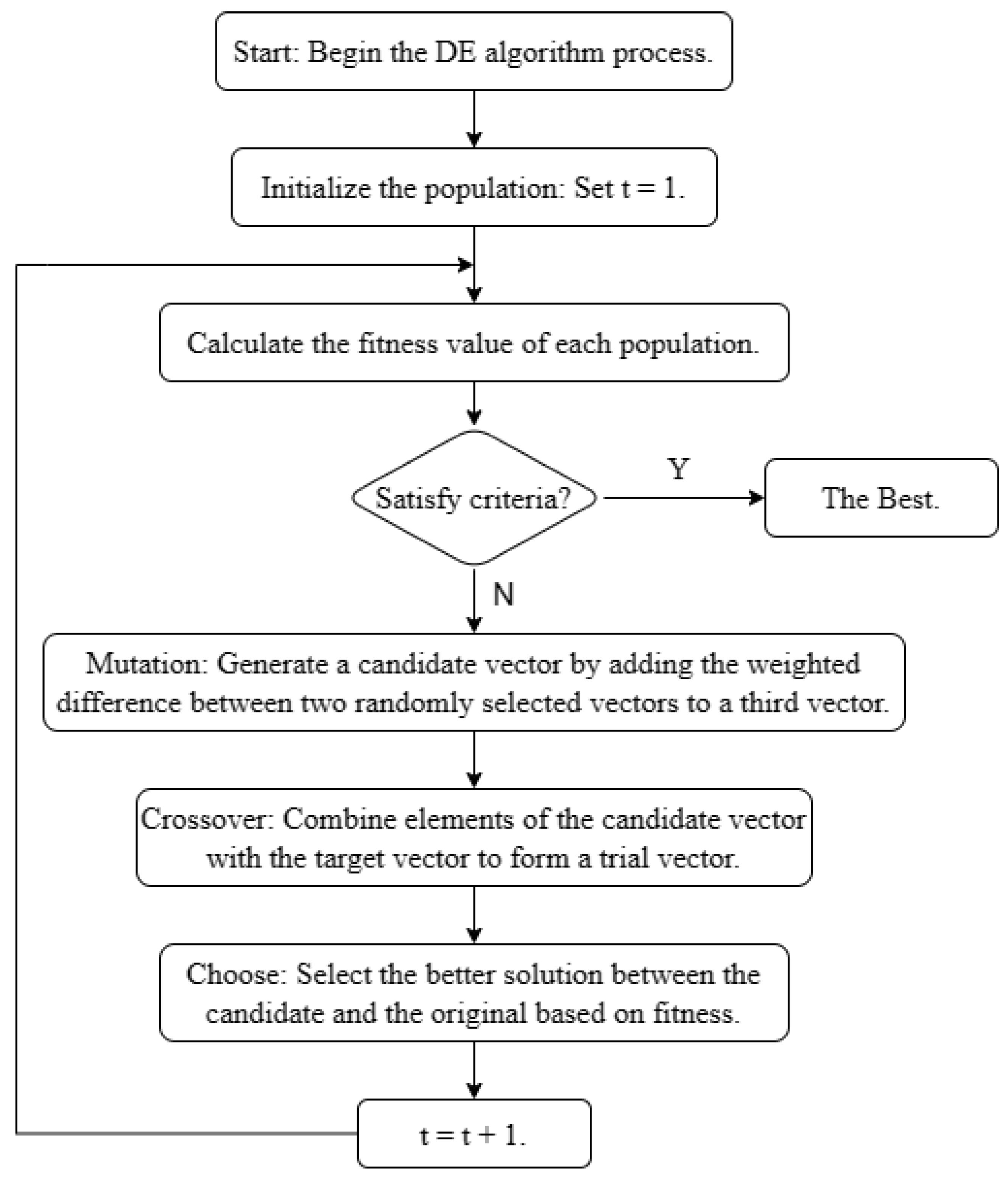
In this section, we outline and describe the steps of the GP surrogate-assisted Differential Evolution (DE) algorithm. The algorithm applies to problems with any number of dimensions n and any number of constraints m. The steps are as follows:
Step 1: Design of Experiments (DOE)
Initialize the algorithm by assigning samples using the Latin Hypercube Design (LHD). The steps are as follows:
Divide each dimension into intervals of equal probability.
Randomly assign one value to each interval within each dimension.
For each dimension, permute the vector of assigned values randomly.
Combine the permuted vectors of assigned values across dimensions into a matrix.
Step 2: Identify the Best Point and Assess Feasibility
Extract the objective function values and constraint violation values from the initial samples. Identify the feasible solutions (those with no constraint violations) and select the one with the optimal objective function value as the best feasible solution. If no feasible solutions exist, select the solution with the least constraint violation as the best infeasible solution. Update the data structure with information about the best solution discovered thus far, and return this information along with a feasibility flag.
Step 3: Clustering—Organize Tested Points into Clusters
Given
N tested points
, if
(where
is the maximum number of points a local model can contain), use all the points to build a single local model. If
, apply fuzzy clustering to divide the points into
clusters, where
and
(where
is the number of points for adding one more local model). The clustering minimizes the following function
J:
where
is a constant greater than 1,
is the centre of the cluster
j,
represents the membership degree of
in cluster
j, and
denotes the Euclidean norm.
can be calculated as
Initialize
for
and
, and set
. Compute
using
If , terminate and output and ; otherwise, increment t and recalculate and until the stopping criterion is satisfied.
Step 4: Modelling—Build Local GP Surrogate Models
For each cluster, construct local Gaussian Process (GP) surrogate models for the objective function and the constraint functions separately.
Step 5: Differential Evolution–Generate and Evaluate Candidate Points
Use Differential Evolution (DE) [
27] to generate
candidate points and evaluate them using the surrogate models. DE is a population-based optimization algorithm that aims to find the global minimum of a given objective function within a high-dimensional search space. The algorithm employs mutation, crossover, and selection strategies to evolve the population towards the optimal solution. During the mutation step, new candidate solutions are generated by combining existing solutions with a weighted difference vector, where the scaling factor is denoted by
F. In the crossover step, these candidates are combined with the original population to form a trial population, with a defined crossover probability
.
Incorporate the Constrained Expected Improvement (CEI) and Constrained Expected Prediction Error (CEPE) criteria, derived from the Gaussian Process (GP) surrogate models, into the evaluation process of candidate points. By computing the CEI and CEPE values for each candidate point, the algorithm leverages these metrics to guide the selection process within DE. Candidate points are prioritized based on higher CEI values, indicating a greater expected improvement, or lower CEPE values, signifying a lower prediction error. This strategic prioritization ensures the exploration of regions in the search space with the highest potential for improvement while adhering to the constraints. This iterative process continues until a termination criterion is met, such as reaching the maximum number of generations
or achieving a predetermined level of convergence. The flowchart of the DE algorithm, highlighting the integration of CEI and CEPE, is depicted in
Figure 1.
Step 6: Evaluation—Use Original Objective and Constraint Functions
Evaluate the candidate points using the original objective and constraint functions. This step can also be considered as the final selection step of Differential Evolution.
Step 7: Iteration—Update Data and Repeat Steps 3 to 6
Incorporate new data from the observations into the model, and repeat Steps 3 to 6 until the termination condition is reached. The termination condition is typically based on the number of function evaluations, denoted as .
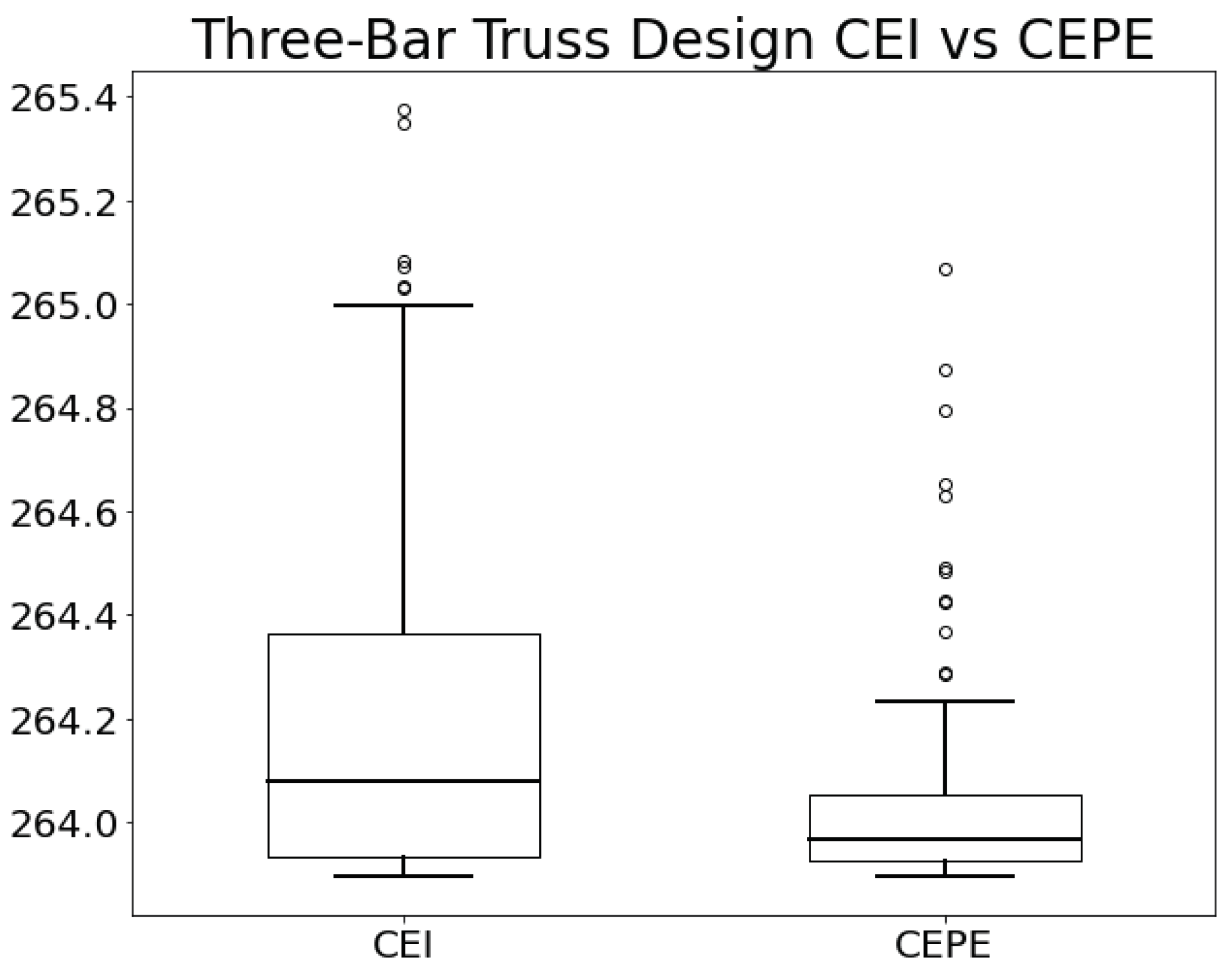
5. Application
In this section, we will apply the GP surrogate-assisted DE algorithm to the Three-Bar Truss Design problem. The Three-Bar Truss Design problem [
30,
31] is a classical optimization problem that is widely studied within the engineering and mathematical communities. The objective is to design a truss structure, composed of three bars, capable of withstanding a specified load while minimizing weight. This problem is particularly significant in the design of lightweight and efficient structures in fields such as aerospace and civil engineering. Moreover, it serves as a quintessential example of how optimization algorithms can address complex societal and civilizational challenges. The problem can be formulated as follows:
where
and
;
cm,
KN/
, and
KN/cm
.
For the experiment, we employ the same parameter settings as in the numerical simulations. The problem has two dimensions and three constraints. Using Latin hypercube design (LHD), we generate 21 initial samples for our population size. The parameters in the fuzzy cluster are set to , , , and . In Differential Evolution (DE), the population size is assumed to be , the number of generations is set to 500, the crossover probability is , and the scaling factor is . In the CEPE method, we set the candidate number to 100. The number of function evaluations (FEs) is 100. The experiment is repeated 100 times using two different methodologies (CEI and CEPE), and the parameters are kept the same to ensure a fair comparison.
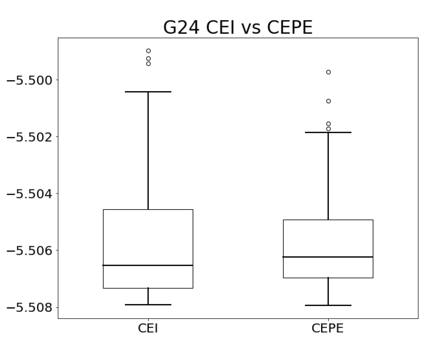
Figure 3 depicts box plots that display the distribution of the objective function values obtained using the CEI and CEPE methods across 100 independent experiments.
Table 5 lists the mean, standard deviation (sd), best, and worst of the objective function values obtained by both methods over 100 iterations. The best-known result for this problem is approximately
. From the table, it is evident that CEPE performs better in terms of mean, standard deviation, and worst objective function values, while CEI marginally outperforms CEPE in the best objective function value.
Additionally, we employ the Wilcoxon rank-sum test to statistically compare the performance of the CEI and CEPE methods. With a p-value of 0.0538%, the test indicates that the CEPE method is significantly superior to the CEI method.
6. Discussion and Remarks
In this paper, we introduced the formulation of constrained optimization problems, the methodologies of Constrained Expected Improvement (CEI) and Constrained Expected Prediction Error (CEPE) in conjunction with the Gaussian Process (GP) surrogate-assisted Differential Evolution (DE) algorithm, and presented numerical benchmark simulations and applications. Additionally, we would like to emphasize the potential application of these methodologies in the field of engineering, where optimization plays a crucial role.
The implementation of CEI and CEPE has showcased their capacity for the efficient utilization of computational resources, making them highly advantageous in engineering contexts where simulation models can be computationally demanding. Their adeptness in managing multiple constraints, robustness against uncertainties, and flexibility to adapt to various problem domains highlight the methodologies’ applicability in real-world engineering problems. These attributes facilitate the optimization of processes, enhancement of product yields, reduction of waste, and improvement in safety and environmental performance.
Despite these advantages, the methodologies do present limitations, such as potential inflexibility in highly specialized engineering challenges and sensitivity to parameter configuration, which could impact their effectiveness. Moreover, the computational intensity required by CEI and CEPE, especially for large-scale problems, warrants consideration. These limitations suggest a cautious approach to their application, emphasizing the need for tailoring or integrating them with other techniques to meet specific engineering requirements.
In summary, the findings from this study affirm the promise of CEI and CEPE in advancing surrogate-assisted optimization strategies for engineering applications. While addressing the identified gaps in constrained optimization, this research also paves the way for future investigations into more sophisticated surrogate models and optimization techniques. Further exploration in this domain could yield even more robust and efficient solutions for complex optimization challenges, contributing to the continuous advancement of engineering optimization practices.


