Abstract
An effective strategy to enhance the convergence order of nodal approximations in interpolation or PDE problems is to increase the size of the stencil, albeit at the cost of increased computational burden. In this study, our goal is to improve the convergence orders for approximating the first and second derivatives of sufficiently differentiable functions using the radial basis function-generated Hermite finite-difference (RBF-HFD) scheme. By utilizing only three equally spaced points in 1D, we are able to boost the convergence rate to four. Extensive tests have been conducted to demonstrate the effectiveness of the proposed theoretical weighting coefficients in solving interpolation and PDE problems.
Keywords:
radial basis function (RBF); convergence order; Hermite finite difference (HFD); analytical weights; fractional PDE MSC:
41A25; 65M22; 35R11
1. Introduction
1.1. Goals
The use of radial basis functions (RBFs) offers several advantages in various applications [1] (Chapters 1–2). RBFs are commonly used for interpolation problems, where they approximate a function based on a set of input–output data pairs. Compared to other interpolation methods, RBFs provide more accurate approximations in high-dimensional spaces [2]. RBFs [3] (Chapter 3) have received interest from researchers in both engineering [4,5] and scientific domains [6,7]. They can also be employed for function approximation problems, where the target is to find a function that models the input–output relationship of a given system. In fact, they can consider both global and local features of the function being approximated, allowing for more accurate predictions. Furthermore, RBFs can model non-linear relationships between input and output variables, making them appropriate for applications where linear models are not sufficient. This flexibility arises from the choice of non-linear basis functions used in RBFs [8,9].
This paper investigates how to improve the computational efficiency and, especially, the convergence order of approximations without increasing the stencil size. In fact, in most already published works in the literature [10,11], to increase the convergence order in 1D based on equally spaced nodes, the convergence order cannot be bigger than two when the stencil size is three, which means the only remaining way to boost the convergence order is to increase the stencil size and consider four or more discretization points in a stencil. Hence, the objective is to achieve improved convergence rates and, thus, to propose compact formulas under the Hermite finite-difference (HFD) approach. Thus, we pursue obtaining the RBF-HFD weights. The objective is to compute analytical coefficients and local truncation errors (LTEs) for these compact formulas, focusing on the 1st derivative and the 2nd derivative.
1.2. Background and Challenges
In the dimension d, a kernel as a RBF can be expressed as , where is the radius and stands for the two-norm. The RBF-FD extends classical FD methods to accommodate scattered node configurations [12]. The method employs RBFs to perform a local approximation of a linear differential operator within a selected neighborhood. This neighborhood, known as the stencil for a specific point, is often determined by the closest neighbors. The RBF-FD has undergone extensive investigation and demonstrated successful performance across various contexts; see [13] for more. Like the FD methodology, the RBF-FD methodology provides an approximation to a differential linear operator at a specific point by forming a linear summation of at the n nearest knots as follows [14] (Page 70):
In the RBF-FD procedure, the function v can be either a scalar or a vector-valued function, and the weights associated with the RBF-FD need to be calculated. In the initial stages of RBF-FD research, smooth RBFs (infinitely) such as the multiquadric (MQ) as
or the Gaussian as
had been commonly employed (c represents the shape parameter) [15,16].
To enhance the applicability and usefulness of the RBF-FD methodology, one approach is to increase the number of stencil knots. Increasing the number of stencil knots in RBF-FD methods can improve the stability, the convergence, and the method’s accuracy, but it can also increase the computational cost and sensitivity to noise.
1.3. Motivation
Recently, Fornberg proposed an efficient algorithm in [17] to compute the compact weights for different node layouts. The authors in the work [18] introduced a unified framework for the systematic derivation of optimized compact formulas tailored for uniform grids. These schemes are computed analytically through the solution of an optimization problem, with the objective of minimizing the error while satisfying prescribed accuracy constraints. Furthermore, it demonstrates the versatility of this framework by showing its ability to generate various types of formulas, including spatially explicit and FD formulas, as special cases.
In this work, we study how to improve the convergence order without increasing the stencil size. So, the motivation is to obtain a higher order of convergence using only three-node stencils. Thus, we propose a new set of weights under a variant of the MQ RBF.
1.4. Structure
We provide the rest of the manuscript as follows. In Section 2, the RBF-HFD scheme is furnished. Section 3 is devoted to approximate the 1st and 2nd function derivatives in 1D. The theoretical error equations corresponding to the RBF-HFD formulations under a variant of the MQ RBF are provided therein as well. In Section 4, we substantiate the validity, convergence, and precision of the constructed formulas via several experiments based on LTEs. Section 5 gives one application when the obtained set of weights can be used in solving a fractional time-dependent partial differential equation (PDE). Finally, Section 6 is devoted to drawing a short conclusion of the paper, offering a summary of the obtained results.
2. RBF-HFD Formulations
To improve the convergence results while avoiding the increase of the stencil size, Wright and Fornberg [19] discussed a compact method via Hermite RBF interpolation called the RBF-HFD scheme. The RBF-HFD scheme includes not only the nodal functional values, but also their derivatives. This allows the compact FD to achieve higher accuracy in solving PDEs, particularly in problems with steep gradients or singularities. See [20,21] for more.
We now describe the RBF-HFD as follows. The computation of the operator at involves examining a stencil comprising nodes in dimension one, as expressed in the following relation [22]:
In this work, and . The determination of the weights in this approach, represented by and , is accomplished through the use of Hermite RBF interpolants, as outlined below:
Moreover, the weighting coefficients can be acquired by solving the ensuing linear system of equations, which emerges upon substituting (3) into (2) and expressing
In (3), the coefficients are functions of c and h. Here, we explore the coefficients of the RBF-HFD scheme via a variant of the MQ RBF furnished as:
3. Finding the Coefficients and the Solution Scheme
The importance of the weighting coefficients in RBF-HFD approximations resides in their capacity to enhance the speed when estimating the 1st and 2nd derivatives with just three neighboring equidistant nodes. By incorporating the Hermite concept, this approach considers not only the functional values at each adjacent point, but also considers the differentiations.
Initially, we examine a collection of evenly spaced points , subsequently applying a three-point stencil organized as follows:
Now, let us examine the RBF-HFD approximation (shown by ) as follows:
To start, we substitute v using (6) at the stencil points, resulting in the subsequent system of equations:
By resolving (9)–(13) through incorporating certain simplifications, we arrive at:
Here, we note that the weights (14)–(16) have been derived through simplifications and Taylor expansions up to the second order of the solution of the linear system (9)–(13). While it is conceivable to consider higher order terms, they result in a more intricate version of the final analytical weights without affecting the ultimate error equation of the approximations, as will be demonstrated in Theorem 1. To elaborate further, expanding the Taylor series up to third- and fourth-degree terms would yield the following equivalent weighting coefficients (respectively):
and
Theorem 1.
Proof.
As explained in Section 2, we obtain the analytical weights for the first derivative using symbolic calculations. The set of weights (14)–(16) would yield in the following LTE:
where
The equation of error (23) shows a quartical convergence rate for the presented approximation on uniformly spaced grids. The details of the proof can be extracted from the Mathematica program given in Appendix A. This concludes the proof. □
In tackling the situation related to the second derivative as outlined in Section 2 within the RBF-HFD approach, we utilize (7) and express:
We used different symbols and for the coefficients to differ in contrast to the first derivative approximation. Likewise, by formulating the subsequent set of five interrelated equations at the nodes of the stencil:
Solving the system (26)–(30) results in the following solution:
Here, it is mentioned that the weights (31)–(33) have been figured out by making the formulas simpler and using Taylor expansions up to the second order of the solution of the linear system (26)–(30). Although we could think about using higher order terms, doing so would make the final analytical weights more complex without making a difference for the error equation of the approximation, as we will show in Theorem 2. For example, if we consider the Taylor expansion up to fourth-order terms, we obtain:
Theorem 2.
Proof.
By incorporating the Taylor series having the second truncation order for the coefficients and putting them back in (25), it is finally obtained:
Here,
The relation (37) reveals a quartic convergence speed for the second derivative of an sufficiently differentiable function, using a three-node stencil. This concludes the proof. □
4. The Advantage of the Analytical Coefficients
To affirm the precision of our formulas and examine how the LTE relies on h and c, we employed the subsequent test functions as illustrative instances:
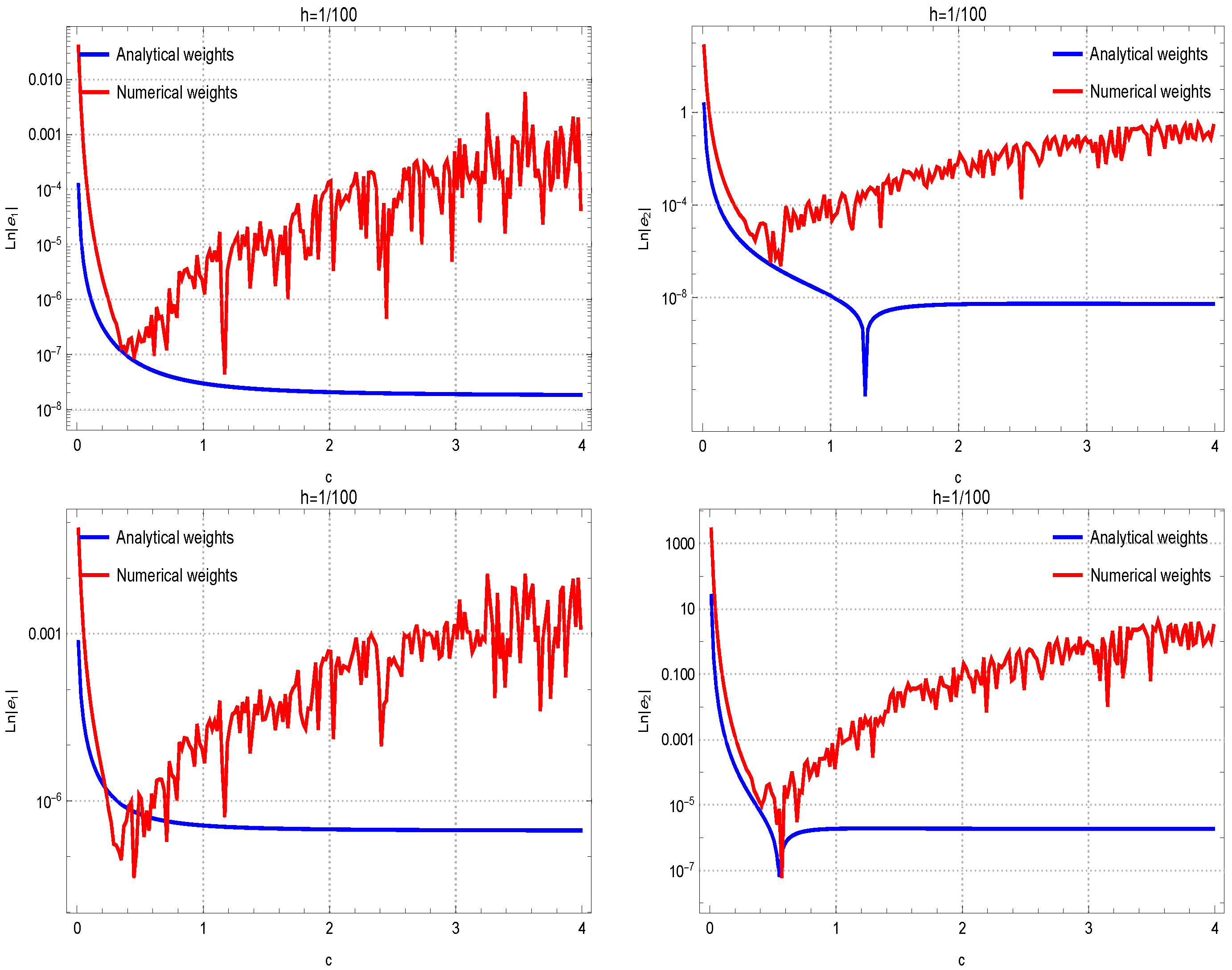
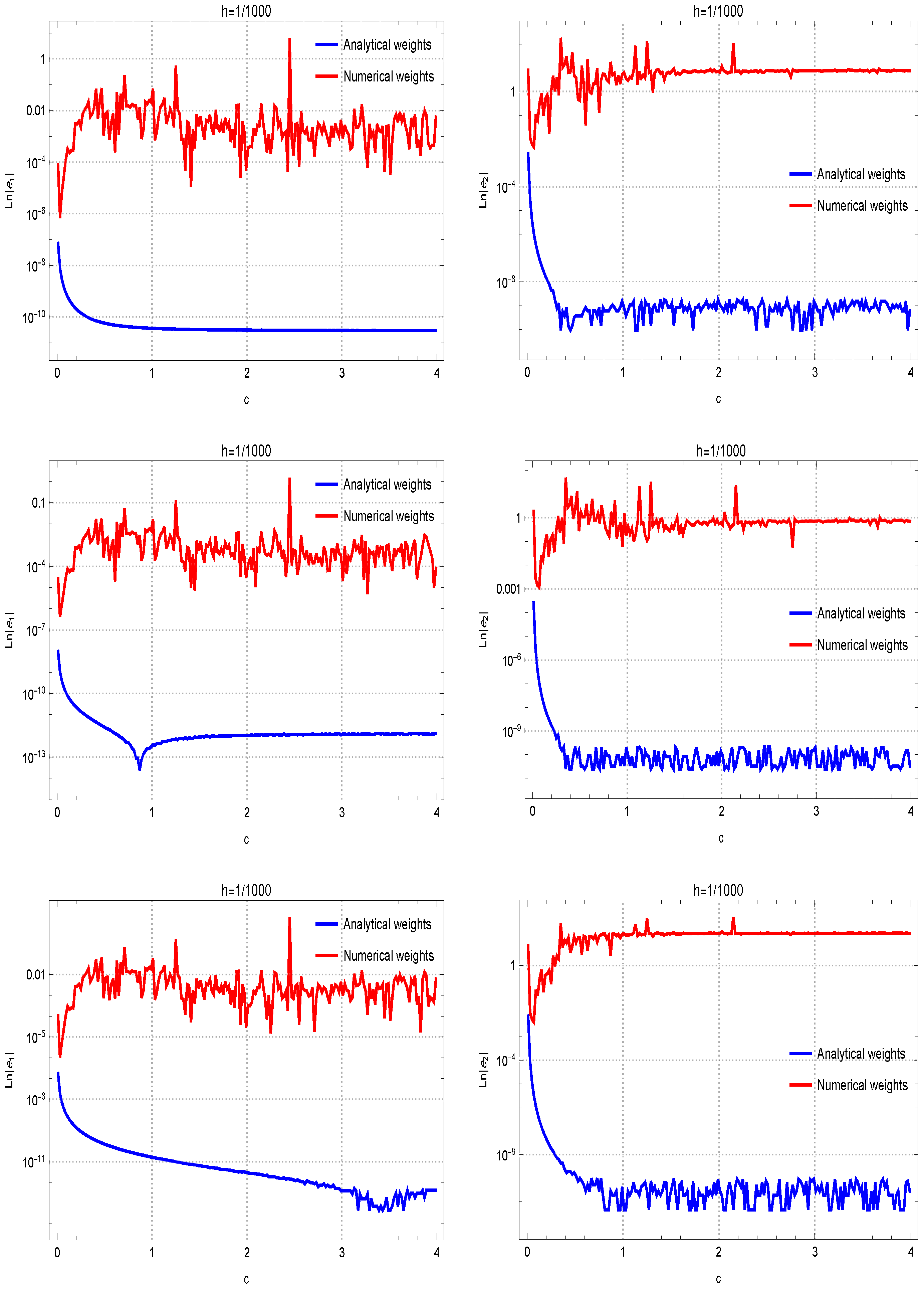
To attain this objective using , we employ (7) in conjunction with Formulas (14)–(16) to approximate the first derivatives. The subsequent findings, depicted in Figure 1, reveal the enhanced efficacy of theoretical coefficients when dealing with (9)–(13). This superiority becomes apparent in the absence of undesired oscillations and the considerable reduction of absolute errors (AEs). In contrast, computational weighting coefficients show divergence attributed to round-off errors, while theoretical weighting coefficients demonstrate stability.

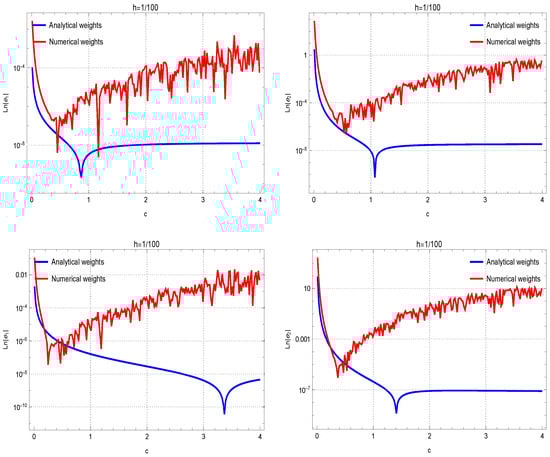
Figure 1.
Evaluating the accuracy of theoretical coefficients against numerical weights is conducted across test functions , …, , organized in rows 1 through 4. The assessment is performed with the fixed . The outcomes for approximating the first and second derivatives are given in the left and right figures, respectively.
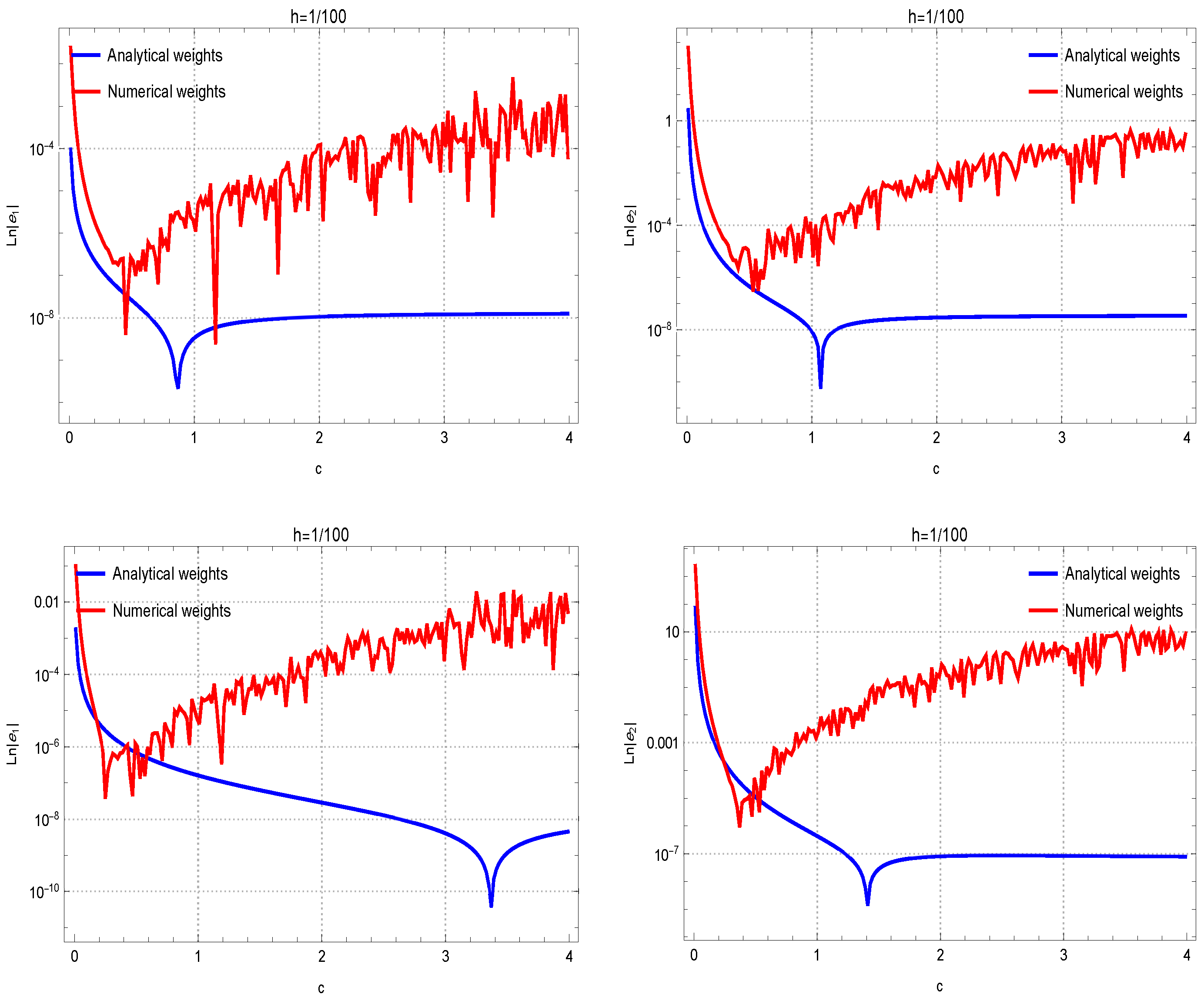
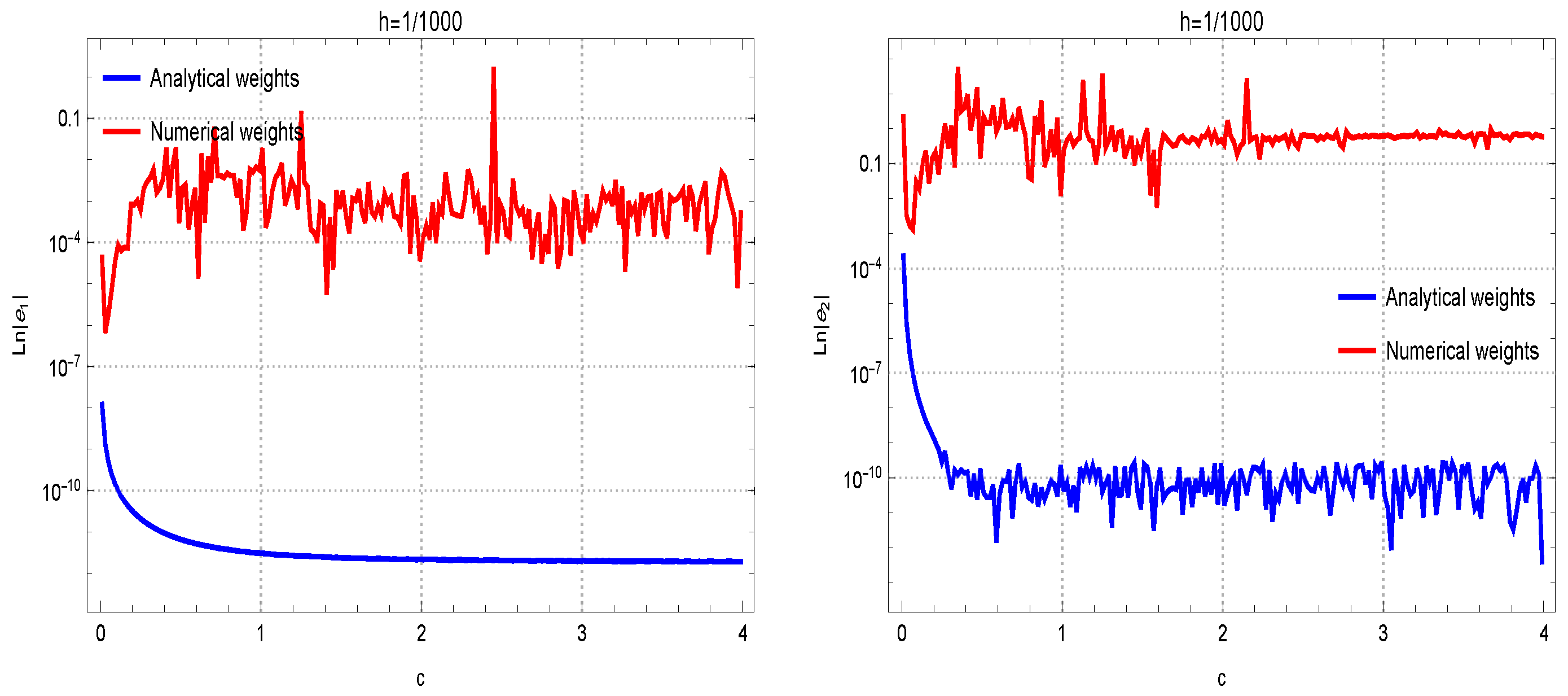
Another exploration was undertaken to show the capabilities of (31)–(33) for estimating the second derivatives, comparing their performance to their numerical counterparts. The results presented in Figure 2, when , offer additional affirmation of the advantages of theoretical coefficients in this context. Discrepancies in the performance of the method for first and second derivatives at different grid spacings ( and ) can be observed in the results. In fact, the lower the grid spacing is, more accurate results in terms of absolute errors can be observed.
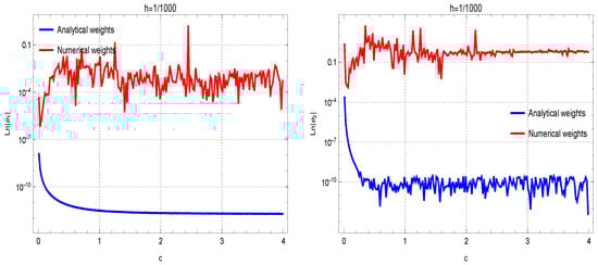
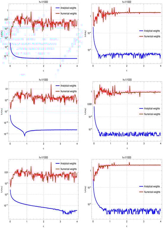
Figure 2.
Evaluations of the accuracy of theoretical coefficients against numerical weights are conducted across test functions , …, organized in rows 1 through 4. The assessment is performed with the fixed . The results for approximating the first and second derivatives are given in the left and right figures, respectively.
The gap observed between analytical and numerical weights in Figure 2 requires further explanation. The insights into the factors contributing to this difference is necessary to ensure a thorough understanding of the results. The main reason lies in solving the linear systems in machine precision, which introduces round-off and cancellation errors especially when h tends to zero or c tends to be very large. In such cases, the linear system is ill-conditioned. However, solving the system in exact arithmetic and using the analytical weights can diminish such errors in computing.
Checking the Rate of Convergence
The numerical order of convergence (NOC) is investigated using the absolute error (under the discretization step size h) and can be defined as follows:
The test for checking the NOC is as follows:
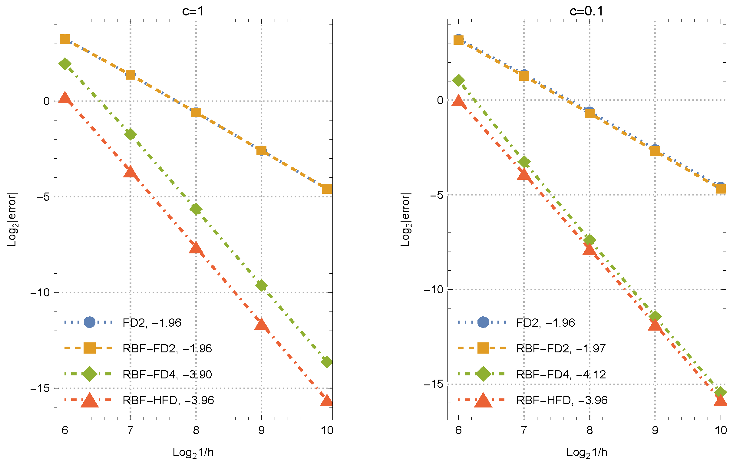
The convergence behavior and NOCs for four different approximations are presented in Figure 3. We approximate the first derivative of the function (44) at . The compared methods on equi-spaced grids are the three-point FD, RBF-FD, and five-point RBF-FD weights given in [23]. The proposed weights (14)–(16) are shown by RBF-HFD. The slope corresponding to each set of weights obtained is reported next to the caption of each method in Figure 3. Noting that the comparison of the weights with a small shape parameter against those with a large shape parameter lacks justification, due to this, we have chosen different shape parameters, but the same for all methods when comparing. The results confirm the theoretical orders of Section 3.
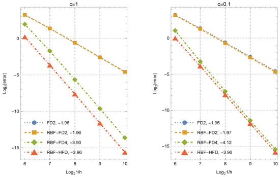
Figure 3.
NOCs for various sets of weights in approximating the first derivative.
5. A PDE Problem
The time-dependent fractional Black–Scholes (FBS) PDE presents numerous advantages in options pricing within financial markets when compared to the conventional BS equation [24]. This formulation, applicable for , is expressed as follows [25]:
where , t represents the time to maturity, and r denotes the interest rate, while additional parameters include for dividend yield and for the volatility constant. Furthermore, expressing as indicates the actual Hurst exponent as , as established in [26]. It is observed that Equation (45) simplifies to the classical Black–Scholes partial differential equation (BS PDE) when . If we designate E as the price of the strike, the initial condition for (45) can alternatively be characterized for the call and put variations [27,28]:
and
The boundary conditions for call/put options are expressed, respectively, by
Here, the errors are documented and subjected to comparison. The methods we used for the comparisons are as follows:
- The method based on the introduced RBF-HFD weights in Section 3 and shown by PM.
- The 2nd-order FD solver on equally spaced meshes and 1st-order Euler’s method along time [29] shown by FD2.
- The RBF-FD approach on uniformly spaced grids is employed to tackle (45), as discussed in [30]. In this section, we denote it as SSM.
Mathematica 13.3 [31,32] is used to perform the computations in standard floating point arithmetic. Here, is considered. Note that the proposed sets of weights are employed on uniform Cartesian meshes. This is done intentionally to gain as much as possible of the convergence order in practical problems. So, we do not employ non-Cartesian nodes for solving (45), which are unnecessary for this problem.
The shape parameter for any of the kernels is chosen adaptively as follows:
The error is given by while and denote the reference and computational solutions, respectively. The computations were conducted on a system with Windows 11 and an Intel Core i7-9750H processor. The time required for these computations, measured in seconds, is presented in the tables under the label .
We analyzed a call option possessing the spot price of USD 100, by considering that today is 13 February 2024 and the option expires on 13 February 2025. The annualized rate of interest is 5%, with an annualized volatility of 40%, and equals 0. Additionally, , and is established, as mentioned in [30]. This value serves as a benchmark for comparisons. The following section provides a detailed set of computational comparisons involving various solvers. Table 1 illustrates a comparison of various solvers for solving (45).

Table 1.
Results among various solvers in Section 5.
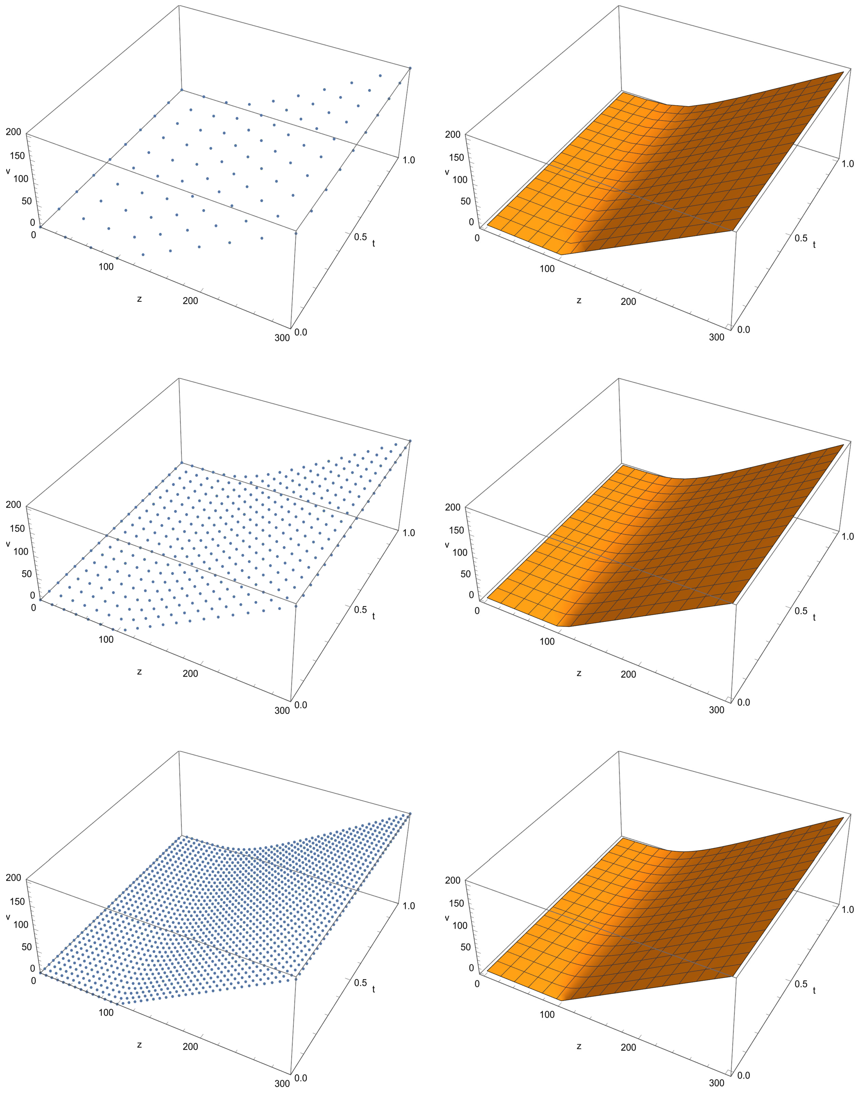
Three solvers were evaluated: the FD2, SSM, and PM schemes. The proposed scheme performed much better than the other methods in terms of both accuracy and efficiency. To evaluate its stability and positivity, we investigated the numerical solution with varying numbers of discretized points across the interval, as illustrated in Figure 4. The figure presents computational solutions using three sets of uniform points. The left subplots showcase the discrete computational resolutions, while the right ones display the continuous versions extracted through interpolation, produced by the programming package.
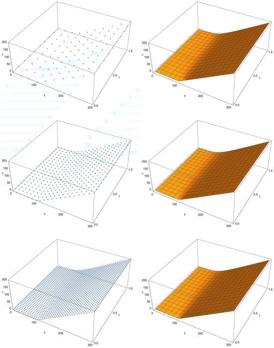
Figure 4.
Numerical findings upon solving FBS PDE by PM. Upper left: A plot illustrating the situation having . Upper right: A plot of the solution having . Middle left: A point plot via . Middle right: A continuous plot showing the setup having . Lower left: A point plot showing the scenario having . Lower right: A continuous plot showing the configuration having .
However, here, we note that the proposed methodology has a drawback of being employed in arbitrary domains for scattered node layouts. In fact, since it requires the Hermite condition, i.e., the derivative information for each point of the stencil except the center, then such information might be unavailable to time-consuming in arbitrary domain problems, which might restrict its application. So, it mainly is suitable for interpolations, as well as for PDE problems on regular domains.
6. Conclusions
This study proposes coefficients for the RBF-HFD methodology using a variant of the multiquadric (MQ) RBF to approximate the 1st and 2nd derivatives of a function. The analytical computation of weights and LTEs highlights the efficiency of this methodology. Computational results confirm the effectiveness of this approach, indicating its potential for various applications in numerical analysis and solving PDE problems. Future research will focus on enhancing the convergence order on a stencil with five nodes using the RBF-HFD approach, comparing it to the convergence rates of FD or RBF-FD approximations on such a stencil. Additionally, exploration will be conducted on applying this strategy to the state-of-the-art polyharmonic spline (PHS) RBF, which is parameter-free.
Author Contributions
Supervision, T.L. and S.S.; methodology, T.L. and S.S.; investigation, T.L. and S.S.; funding acquisition, T.L. and S.S.; formal analysis, T.L. and S.S.; conceptualization, T.L. and S.S.; validation, T.L. and S.S.; writing—original draft, T.L. and S.S.; writing—review and editing, T.L. and S.S. All authors have read and agreed to the published version of the manuscript.
Funding
The research of the first author was funded by the Research Project on Graduate Education and Teaching Reform of Hebei Province of China (YJG2024133).
Data Availability Statement
No new data were created or analyzed in this study.
Conflicts of Interest
The authors declare no conflicts of interest.
Appendix A
The Mathematica 13.0 program used in the process of the proof in Theorem 1.
ClearAll["Global`*"];
ph[r1_] := (c^2 + r1^2)^(3/2)
F1 = D[ph[r1], r1] // FullSimplify;
F2 = D[ph[r1], {r1, 2}] // FullSimplify;
v1[z_] := a1*v[z - h] + a2*v[z] + a3*v[z + h] + b1*v’[z - h] + b2*v’[z + h]
(*First derivative*)
eq1 = ((F1 /. {r1 -> -h}) == {(ph[r1] /. {r1 -> -2 h}), (ph[
r1] /. {r1 -> -h}), (ph[r1] /. {r1 -> 0})
, (F1 /. {r1 -> -2 h}), (F1 /. {r1 -> 0})} . {a1, a2, a3, b1,
b2}) // Simplify;
eq2 = ((F1 /. {r1 ->
0}) == {(ph[r1] /. {r1 -> -h}), (ph[r1] /. {r1 -> 0}), (ph[
r1] /. {r1 -> h})
, (F1 /. {r1 -> -h}), (F1 /. {r1 -> h})} . {a1, a2, a3, b1,
b2}) // Simplify;
eq3 = ((F1 /. {r1 ->
h}) == {(ph[r1] /. {r1 -> 0}), (ph[r1] /. {r1 -> h}), (ph[
r1] /. {r1 -> 2 h})
, (F1 /. {r1 -> 0}), (F1 /. {r1 -> 2 h})} . {a1, a2, a3, b1,
b2}) // Simplify;
eq4 = ((F2 /. {r1 -> -h}) == {(F1 /. {r1 -> -2 h}), (F1 /. {r1 -> \
-h}), (F1 /. {r1 -> 0})
, (F2 /. {r1 -> -2 h}), (F2 /. {r1 -> 0})} . {a1, a2, a3, b1,
b2}) // Simplify;
eq5 = ((F2 /. {r1 ->
h}) == {(F1 /. {r1 -> 0}), (F1 /. {r1 -> h}), (F1 /. {r1 ->
2 h})
, (F2 /. {r1 -> 0}), (F2 /. {r1 -> 2 h})} . {a1, a2, a3, b1,
b2}) // Simplify;
{b, A} = Simplify@
CoefficientArrays[{eq1, eq2, eq3, eq4, eq5}, {a1, a2, a3, b1, b2}];
sol = Simplify@(Inverse[A] . (-b));
taylororder = 2;
sol2 = (Normal@Series[Simplify@(sol /. Thread[h -> ep*c]), {ep, 0,
taylororder}] /. ep -> h/c) // FullSimplify
(Series[v1[z] /. {a1 -> sol2[[1]], a2 -> sol2[[2]], a3 -> sol2[[3]],
b1 -> sol2[[4]], b2 -> sol2[[5]]}, {h, 0, 4}] // FullSimplify)
References
- Fasshauer, G.E. Meshfree Approximation Methods with Matlab; World Scientific, 5 Toh Tuck Link: Singapore, 2007. [Google Scholar]
- Fornberg, B.; Flyer, N. Solving PDEs with radial basis functions. Acta Numer. 2015, 24, 215–258. [Google Scholar] [CrossRef]
- Iske, A. Multiresolution Methods in Scattered Data Modelling, Lecture Notes in Computational Science and Engineering; Springer: Heidelberg, Germany, 2004; Volume 37. [Google Scholar]
- Babayar-Razlighi, B. Numerical solution of an influenza model with vaccination and antiviral treatment by the Newton-Chebyshev polynomial method. J. Math. Model. 2023, 11, 103–116. [Google Scholar]
- Ebrahimijahan, A.; Dehghan, M.; Abbaszadeh, M. Simulation of the incompressible Navier-Stokes via integrated radial basis function based on finite difference scheme. Eng. Comput. 2022, 38, 5069–5090. [Google Scholar] [CrossRef]
- Itkin, A.; Soleymani, F. Four-factor model of quanto CDS with jumps-at-default and stochastic recovery. J. Comput. Sci. 2021, 54, 101434. [Google Scholar] [CrossRef]
- Keshavarzi, C.G.; Ghoreishi, F. Numerical solution of the Allen-Cahn equation by using shifted surface spline radial basis functions, Iran. Numer. Anal. Optim. 2020, 10, 177–196. [Google Scholar]
- Cavoretto, R.; Rossi, A.D. An adaptive residual sub-sampling algorithm for kernel interpolation based on maximum likelihood estimations. J. Comput. Appl. Math. 2023, 418, 114658. [Google Scholar] [CrossRef]
- Cavoretto, R.; Rossi, A.D.; Dell’Accio, F.; Tommaso, F.D.; Siar, N.; Sommariva, A.; Vianello, M. Numerical cubature on scattered data by adaptive interpolation. J. Comput. Appl. Math. 2024, 115793. [Google Scholar] [CrossRef]
- Soleymani, F.; Zhu, S. On a high-order Gaussian radial basis function generated Hermite finite difference method and its application. Calcolo 2021, 58, 50. [Google Scholar] [CrossRef]
- Yang, Y.; Soleymani, F.; Barfeie, M.; Tohidi, E. A radial basis function-Hermite finite difference approach to tackle cash–or–nothing and asset–or–nothing options. J. Comput. Appl. Math. 2020, 368, 112523. [Google Scholar] [CrossRef]
- Bayona, V. An insight into RBF-FD approximations augmented with polynomials. Comput. Math. Appl. 2019, 77, 2337–2353. [Google Scholar] [CrossRef]
- Sanyasiraju, Y.V.S.S.; Chandhini, G. Local radial basis function based gridfree scheme for unsteady incompressible viscous flows. J. Comput. Phys. 2008, 227, 8922–8948. [Google Scholar] [CrossRef]
- Tolstykh, A.I. On using radial basis functions in a “finite difference mode” with applications to elasticity problems. Comput. Mech. 2003, 33, 68–79. [Google Scholar] [CrossRef]
- Cheng, A.H.-D. Multiquadric and its shape parameter—A numerical investigation of error estimate, condition number, and round-off error by arbitrary precision computation. Eng. Anal. Bound. Elem. 2012, 36, 220–239. [Google Scholar] [CrossRef]
- Company, R.; Egorova, V.N.; Jódar, L.; Soleymani, F. A stable local radial basis function method for option pricing problem under the Bates model. Numer. Methods Partial. Differ. Equ. 2019, 35, 1035–1055. [Google Scholar] [CrossRef]
- Fornberg, B. An algorithm for calculating Hermite-based finite difference weights. IMA J. Numer. Anal. 2021, 41, 801–813. [Google Scholar] [CrossRef]
- Deshpande, V.M.; Bhattacharya, R.; Donzis, D.A. A unified framework to generate optimized compact finite difference schemes. J. Comput. Phys. 2021, 432, 110157. [Google Scholar] [CrossRef]
- Wright, G.B.; Fornberg, B. Scattered node compact finite difference-type formulas generated from radial basis functions. J. Comput. Phys. 2006, 212, 99–123. [Google Scholar] [CrossRef]
- Fornberg, B.; Flyer, N. A Primer on Radial Basis Functions with Applications to the Geosciences; SIAM: Philadelphia, PA, USA, 2015. [Google Scholar]
- Lele, S.K. Compact finite difference schemes with spectral-like resolution. J. Comput. Phys. 1992, 103, 16–42. [Google Scholar] [CrossRef]
- Collatz, L. The Numerical Treatment of Differential Equations, 3rd ed.; Springer: Berlin/Heidelberg, Germany, 1966. [Google Scholar]
- Soleymani, F.; Barfeie, M.; Khaksar Haghani, F. Inverse multi-quadric RBF for computing the weights of FD method: Application to American options. Commun. Nonlinear Sci. Numer. Simulat. 2018, 64, 74–88. [Google Scholar] [CrossRef]
- Jumarie, G. Derivation and solutions of some fractional Black-Scholes equations in coarse-grained space and time: Application to Merton’s optimal portfolio. Comput. Math. Appl. 2010, 59, 1142–1164. [Google Scholar] [CrossRef]
- Wyss, W. The fractional Black-Scholes equation. Fract. Calc. Appl. Anal. 2000, 3, 51–62. [Google Scholar]
- Hurst, H.E. Long-term storage capacity of reservoirs. Trans. Amer. Soc. Civil Eng. 1951, 116, 770–799. [Google Scholar] [CrossRef]
- Seydel, R.U. Tools for Computational Finance, 6th ed.; Springer: London, UK, 2017. [Google Scholar]
- Dai, X.; Ullah, Z.M. An efficient higher-order numerical scheme for solving fractional Black-Scholes PDE using analytical weights. Iran. J. Sci. 2024, 48, 423–435. [Google Scholar] [CrossRef]
- Zhang, H.; Liu, F.; Turner, I.; Yang, Q. Numerical solution of the time fractional Black-Scholes model governing European options. Comput. Math. Appl. 2016, 71, 1772–1783. [Google Scholar] [CrossRef]
- Song, Y.; Shateyi, S. Inverse multiquadric function to price financial options under the fractional Black-Scholes model. Fractal Fract. 2022, 6, 599. [Google Scholar] [CrossRef]
- Ruskeepää, H. Mathematica Navigator, 3rd ed.; Academic Press: Burlington, VT, USA, 2009. [Google Scholar]
- Georgakopoulos, N.L. Illustrating Finance Policy with Mathematica; Springer International Publishing: Cham, Switzerland, 2018. [Google Scholar]
Disclaimer/Publisher’s Note: The statements, opinions and data contained in all publications are solely those of the individual author(s) and contributor(s) and not of MDPI and/or the editor(s). MDPI and/or the editor(s) disclaim responsibility for any injury to people or property resulting from any ideas, methods, instructions or products referred to in the content. |
© 2024 by the authors. Licensee MDPI, Basel, Switzerland. This article is an open access article distributed under the terms and conditions of the Creative Commons Attribution (CC BY) license (https://creativecommons.org/licenses/by/4.0/).