Personalized Dynamic Pricing Based on Improved Thompson Sampling

Abstract

This study investigates personalized pricing with demand learning. We first encode consumer-personalized feature information into high-dimensional vectors, then establish the relationship between this feature vector and product demand using a logit model, and finally learn demand parameters through historical transaction data. To address the balance between learning and revenue, we introduce the Thompson Sampling algorithm. Considering the difficulty of Bayesian inference in Thompson Sampling owing to high-dimensional feature vectors, we improve the basic Thompson Sampling by approximating the likelihood function of the logit model with the Pólya-Gamma (PG) distribution and by proposing a Thompson Sampling algorithm based on the PG distribution. To validate the proposed algorithm’s effectiveness, we conduct experiments using both simulated data and real loan data provided by the Columbia University Revenue Management Center. The study results demonstrate that the Thompson Sampling algorithm based on the PG distribution proposed outperforms traditional Laplace approximation methods regarding convergence speed and regret value in both real and simulated data experiments. The real-time personalized pricing algorithm developed here not only enriches the theoretical research of personalized dynamic pricing, but also provides a theoretical basis and guidance for enterprises to implement personalized pricing.

1. Introduction

In the past decade, the rapid development of information technology and the Internet has facilitated online sellers in collecting an abundance of personalized information about consumers, including addresses, educational backgrounds, consumption preferences, and social media activity. For sellers, this information encapsulates numerous factors influencing consumer purchasing intentions. It thereby provides strong support for devising more rational pricing policies. Nevertheless, the challenge lies in how the seller can capture the impact of consumer personal features on product demand and, concurrently, leverage this information in pricing to maximize revenue.

To address the above problem, we constructed a personalized dynamic pricing model with demand learning. Specifically, the seller engages in a process of learning to comprehend the relationship between consumers’ personal features and product demands. Subsequently, based on the learning results, the seller implements a distinct quoted price (i.e., personalized pricing) for consumers with different features. Finally, sellers observe consumers’ purchasing decisions and continue the process of demand learning. Although there have been numerous research achievements in dynamic pricing with demand learning, our problem exhibits two distinct characteristics. Firstly, we depart from the conventional approach by associating consumer’s personalized characteristics with product demand, whereas previous studies have mainly focused on constructing demand models based on product value perspectives or external factors influencing consumer purchasing behavior. Secondly, our dynamic pricing does not entail temporal fluctuations in prices but rather involves setting different prices for individual consumers, known as personalized pricing.

Personalized pricing, due to its significant unfairness as a form of first-degree price discrimination, has sparked considerable controversy. However, numerous academic studies suggest that personalized pricing yields favorable outcomes from the perspectives of firms, consumers, and social welfare [1,2,3]. Dubé and Misra [4] showed that compared to uniform pricing, firms that adopt personalized pricing experience a profit increase exceeding 10%. From a redistributive perspective, personalized pricing proves advantageous for most consumers. They further emphasized that overly restricting companies from utilizing data for personalized pricing may harm consumer interests. Elmachtoub et al. [5] argued that although implementing personalized dynamic pricing is expensive, it is more valuable than uniform pricing. Kolbeinsson et al. [6] collaborated with European Galactic Air to provide ancillaries at dynamic and personalized prices based on flight characteristics and customer demands. The research findings revealed that this policy not only significantly increases the airline’s revenue but also enhances customer satisfaction, achieving a win-win situation. Kallus and Zhou [7] pointed out that personalized pricing generates more welfare benefits. In real business practice, many firms have begun to adopt personalized pricing policies. Expedia tailors have personalized travel product recommendations and price discounts for each user based on their search history, browsing records, booking behavior, membership level, and other personal information. Online retailers like Walmart adjust prices or offer promotional strategies personalized to consumers based on their browsing history, search records, purchase frequency, geographic location, and other information. In the insurance and lending industries, personalized pricing has long been prevalent. When purchasing insurance products, insurance companies determine premiums based on features such as age, gender, health condition, occupation, geographic location, and insurance history. Similarly, when you need a loan for purchasing a car, lending companies determine the final loan interest rate based on your credit rating, credit history, loan amount, loan term, income and employment status, Loan Prime Rate (LPR), and competitor rates. The subsequent problem description, presented in Section 3, is precisely based on applications in the lending industry, and numerical experiments were conducted using real lending industry data for analysis.

The key to personalized pricing is to gain insight into the relationship between consumers’ features and their purchasing decisions. This necessitates continuous learning on the part of sellers. To this end, we consider that a monopolist sells a product in a finite horizon, where consumers arrive sequentially, and the seller can observe consumers’ characteristic information. We employ a logit model to describe the consumer’s decision-making process. The model parameters capture the joint impact of consumer features and prices on product demand. At the beginning of each period, the seller sets prices based on arriving consumer features, observes sale outcomes, and updates the model parameters using Bayesian rules. In this learning process, trying additional prices helps in learning the true values of the parameters as soon as possible. However, this may result in a partial loss of revenue. To strike a balance between learning and earning, we employ the widely used Thompson Sampling (TS) algorithm. However, encoding consumer’s personal features into a high-dimensional vector leads to a high-dimensional Bayesian inference for the corresponding parameters, which is very challenging. To address this, we introduce Pólya-Gamma latent variables and propose a TS algorithm based on the Pólya-Gamma distribution.

This study’s main findings and contributions are threefold. First, we investigate the dynamic pricing problem with demand learning. Compared with problems in the existing literature, the problem in this study is more complex, mainly in the sense that the demand function is jointly affected by consumers’ personal features and prices. Since the consumer’s personal features are encoded as a high-dimensional vector, the demand learning in this study is a high-dimensional Bayesian inference problem, treated as a difficult problem in academia. Second, we propose a personalized dynamic pricing algorithm with improved TS. Compared with the general TS algorithm, the algorithm proposed in this study has faster convergence and lower regret values. Finally, the personalized pricing strategy studied in this study can provide useful lessons for business operations.

The remainder of this paper is organized as follows. Section 2 reviews the relevant literature. Section 3 introduces the dynamic pricing model incorporating reference prices and extends it to the case of uncertain demand, that is, dynamic pricing based on the reference effect and demand learning. Section 4 describes the approximate solution algorithm for the proposed model. Section 5 presents numerical analyses and discussions. Section 6 concludes the study.

2. Related Literature

Our study relates to the literature on dynamic pricing with demand learning, personalized dynamic pricing, and the multi-armed bandit solution method.

Dynamic pricing with demand learning. Classical dynamic pricing models are built upon deterministic demand functions, where the variables influencing demand and their corresponding coefficients are known. However, in reality, accurately obtaining such information is highly challenging. Therefore, dynamic pricing with demand learning has consistently attracted the attention of numerous scholars in the fields of revenue management and operation management. Den [8] provided a comprehensive review of the origins, development, and future research directions of dynamic pricing with learning. Methodologically, current research on dynamic pricing with demand learning can be classified into two major categories. One involves traditional statistical methods such as maximum likelihood estimation [9,10], least squares estimation [11], and Bayesian estimation [12,13,14]. These methods’ main characteristic is a predetermined form of the demand function. The sellers must learn the function’s parameters, so the methods are often referred to as parametric demand learning. The form of the demand function depends on the specific research question. Another category gaining popularity recently is machine learning methods for demand estimation [15,16,17]. A substitution effect among multiple products in the Fast-Moving Consumer Goods industry will significantly affect product demand forecasting. Lee et al. [18] utilized the latest machine learning algorithms to perform the selection of a multi-product demand prediction model that considers the substitution effect. Cai et al. [19] used a deep learning method and demonstrated the positive performance of a deep learning-based choice model with real data. Spiliotis et al. [20] compared the differences between statistical and machine learning methods in demand forecasting. Other research has combined demand learning with factors that impose constraints on pricing optimization, such as reference effects [21,22], inventory control [23], discounting [24], and assortment optimization [25].

Most of the above literature used price as the sole variable affecting demand. This study incorporates both consumer’s personal characteristics and price into the factors influencing demand; the consumer’s personal characteristics are encoded into a high-dimensional vector, making the parameter estimation of the demand function more complicated.

Personalized dynamic pricing. Over the past decade, the rapid development of industries such as information storage, cloud computing, and the Internet has provided technological support for implementing personalized pricing. Many scholars have also begun to research personalized pricing. Aydin and Ziya [1] assumed that consumers provide a signal about their individual willingness to pay when they arrive to conduct business and that firms can apply fully personalized pricing and partially personalized pricing based on this signal. They found that in the fully personalized pricing model, the optimal price is monotonic concerning the signal, while in the partially personalized pricing model, the optimal price policy is of a threshold type. Chen et al. [26] investigated the impact of consumer participation in identity management on firm profits, consumer surplus, and social welfare when a firm implements personalized pricing. Steinberg [27] pointed out that firms utilizing big data for personalized pricing can increase social welfare and contribute to a better state of affairs regarding both welfare and resource equality. Rhodes and Zhou [28] explored the impact of personalized pricing on firms under different market structures. They found that in a fixed market structure, personalized pricing intensifies competition if there are many purchasing consumers in the market, thereby harming company profits. When there are fewer purchasing consumers in the market, personalized pricing is not advantageous for consumers. When the market structure is endogenous, personalized pricing is always beneficial to consumers. While substantial research has demonstrated the advantages of personalized pricing for consumers and social welfare, concerns related to fairness and other aspects of business ethics arise because of severe price discrimination. Seele et al. [29] provided an overview of the ethical challenges caused by algorithm-based personalized pricing. In addressing the fairness of feature-based price discrimination in a monopoly market, Das et al. [30] introduced a concept called α-fairness, ensuring that individuals with similar characteristics face similar prices. Cohen et al. [31] defined price fairness, demand fairness, consumer surplus fairness, and no-purchase value fairness in price discrimination. They found that applying a moderate amount of price fairness increases social welfare, while excessive implementation may lead to lower welfare compared to not applying fairness. Additionally, imposing demand fairness or consumer surplus fairness always reduces social welfare. Chen et al. [32] investigated the implementation of personalized pricing from the perspective of privacy protection. To mitigate the perceived unfairness among consumers because of personalized pricing, an effective strategy is for firms to set a uniform product price while offering different coupons to consumers, known as personalized promotions. Jagabathula et al. [33] represented products as nodes in a directed acyclic graph, where the directed edges indicated consumer preference order between two products. They constructed a non-parametric choice model for consumers and proposed a back-to-back personalized promotion strategy based on this model. Through testing on real datasets, the aforementioned personalized promotion strategy was found to significantly increase the firm’s revenue. Hallikainen et al. [34] found that personalized price promotions effectively alleviate the negative impact of consumers’ perceived cognitive effort on loyalty. In elucidating the basic purchase probability and consumer trend probability, Baardman et al. [35] developed a new consumer trend demand model, namely, the personalized demand model. They estimated the proposed demand model using historical transaction data, and then established a personalized promotion optimization model. The results revealed that personalized promotion strategies increased the firm’s profit by 3–11%.

The above literature models personalized pricing from the perspective of willingness to pay. This study additionally considered the impact of consumer’s personalized characteristics on demand. Furthermore, we assumed that the relationship between personalized features and demand is unknown.

Solution method of multi-armed bandit (MAB). The MAB problem refers to the challenge of selecting optimal actions to maximize cumulative rewards within limited periods, with the core issue being the balance between exploration and exploitation. Recently, the MAB framework has gained widespread application in various fields, such as recommendation systems [36,37], healthcare [38], and dynamic pricing [39,40,41,42]. Currently, three commonly used algorithms for solving the MAB problem are the $\mathsf{\epsilon }$-greedy algorithm, Upper Confidence Bound (UCB) algorithm, and TS. The $\epsilon$-greedy algorithm refers to an agent randomly choosing a non-greedy action with a small probability $\epsilon$ ($\epsilon >0$) during decision making (i.e., exploring with probability $\epsilon$) and choosing a greedy action with a probability of $1-\epsilon$ (i.e., exploiting with probability $1-\epsilon$). However, this algorithm randomly selects a non-greedy action with equal probability $\epsilon$, which has some blindness and may overlook actions with potentially higher rewards (i.e., actions chosen less frequently). Therefore, scholars developed the UCB algorithm. This algorithm considers the sum of the current action’s reward and uncertainty as the objective function for optimization. This encourages the agent to choose actions with greater uncertainty during exploration. However, the UCB algorithm also has limitations, particularly in handling high-dimensional state spaces. The third commonly used algorithm is TS. Compared to the first two algorithms, TS is a random algorithm that updates the posterior distribution based on each action’s prior distribution and observed data. Then, it samples a parameter from the posterior distribution and chooses the optimal action based on this parameter. TS can fully utilize prior knowledge and has lower computational complexity compared to the first two algorithms. It has also received attention from many scholars. Ferreira et al. [43] considered a price-based network revenue management problem, where a retailer sells a limited inventory of multiple products over a finite period, and proposed a dynamic pricing algorithm based on TS to learn unknown parameters in the demand model. Building on this, Ringbeck and Huchzermeier [44] combined Gaussian processes with the TS algorithm to create a Bayesian framework for demand learning. Miao and Chao [25] proposed a learning algorithm based on TS to solve a joint assortment optimization and pricing problem.

In practical applications, agents often encounter contextual bandit problems, where rewards depend not only on the selected actions, but also on contextual information from the environment. Consequently, numerous scholars have studied algorithms for solving contextual bandit problems. The most prominent focus has been on linear contextual bandits, where rewards are linearly related to the actions and context. Li et al. [45] proposed a LinUCB algorithm, which models rewards as a linear function of actions and context and then selects the optimal action based on the UCB principle. The advantage of this algorithm lies in its simplicity of computation and the ability to obtain rigorous theoretical guarantees. However, it cannot handle nonlinear models. To address this limitation, Zhou et al. [46] introduced the Neural UCB algorithm, which utilizes neural networks to model the reward function, enabling it to adapt to various types of problems, especially more complex ones. However, due to the significant computational resources required for training and inference in neural networks, particularly when dealing with large-scale datasets, the Neural UCB algorithm suffers from high computational complexity. Additionally, the performance of the algorithm is noticeably affected by the hyperparameters in the neural network. When it is challenging to describe the reward function using parameterized models, the Decision Tree Bandit algorithm [47] offers a viable alternative. Its core idea is to use a decision tree to model the relationship between contextual information and rewards and make action selections based on this model. However, the limitation of this algorithm lies in its sensitivity to the data distribution. If the data are noisy, this may lead to a decrease in model performance.

We adopted TS to solve personalized dynamic pricing with demand learning. However, in this study’s context, consumers’ personal characteristics form a high-dimensional vector, presenting a challenge to Bayesian inference. Improvements to the basic TS are required.

3. Problem Description and Model Formulation

Consider a monopolist, hereafter referred to as the seller, that sells a product over a horizon of length T. Consumers arrive sequentially, and only one consumer arrives in each period. When a consumer arrives in period $t$, the seller observes d-dimensional personalized features of the consumer, denoted by $Z_t=\{z_{t1},z_{t2},\dots ,z_{td}\}\in R^d$. We assume that $\{Z_t,t=1,2,\dots ,T\}$ are independent and identically distributed. For the convenience of the subsequent explanations, we define the augmented feature vector $X_t={[1,z_{t1},\dots ,z_{td}]}^T\in R^{d+1}$, where the first element represents the intercept term. Accordingly, we denote the mean and covariance matrix of $X_t$ by $\mu$ and $\Sigma$, where $\Sigma =E[X_t{X}_t^T]$ is a symmetric and positive-definite matrix. In period $t$, the seller first chooses a price $p_t\in [p_{\min },p_{\max }]$ after observing $X_t=x_t$, and then the consumer decides whether to purchase the product. Consequently, demand $D_t$ is jointly influenced by price $p_t$ and feature vector $x_t$. We assume that each consumer purchases at most one product. If the consumer accepts the price $p_t$, then $D_t=1$; otherwise, $D_t=0$. That is, the demand follows a Bernoulli distribution.

Following Ban and Keskin [48], we use the logit demand to describe a consumer’s purchasing decisions,

$$D_t=\{\begin{array}{l}1withprobability\frac{e^{\alpha \cdot x_t+(\beta \cdot x_t)p_t}}{1+e^{\alpha \cdot x_t+(\beta \cdot x_t)p_t}}\\ 0withprobability\frac{1}{1+e^{\alpha \cdot x_t+(\beta \cdot x_t)p_t}},\end{array}$$

(1)

where $\alpha ,\beta \in R^{d+1}$ are vectors of the demand parameters that are fixed and unknown to the seller.

Let $\mathit{\theta }:=(\alpha ,\beta )$, and its range is a compact rectangle $\Theta$ in $R^{2(d+1)}$. Given $\mathit{\theta }\in \Theta$ and $x_t$, the seller’s revenue in period $t$ is

$$r_t(p_t,x_t)=p_t\cdot \frac{e^{\alpha \cdot x_t+(\beta \cdot x_t)p_t}}{1+e^{\alpha \cdot x_t+(\beta \cdot x_t)p_t}}.$$

(2)

The seller’s goal is to dynamically adjust the price $p_t$ to maximize total revenue over the time horizon T. For the sake of analysis, we assume that the product cost is zero and there are no stockouts.

The parameter $\mathit{\theta }$ is unknown, which poses a challenge to the seller’s pricing decision. A common and feasible solution is to learn the parameter $\mathit{\theta }$ through price experiments. Specifically, the seller has a prior belief of $\mathit{\theta }$ and sets the price p_t based on observed consumers’ personal features. Consumers decide whether to accept p_t and make a purchase. The seller then updates the belief of $\mathit{\theta }$ based on the consumer’s purchasing decision. We assume that the seller employs the Bayesian update rule. Clearly, setting additional prices (i.e., exploring) facilitates learning the true value of $\mathit{\theta }$; however, this is impractical in actual operations. On the one hand, the cost of conducting price experiments is high. On the other hand, excessive exploration without fully leveraging current learning results can lead to profit loss. Therefore, the seller must strike a balance between exploration and exploitation; that is, the seller faces an MAB problem.

Currently, the primary common algorithms used to solve MAB problem are the $\epsilon$-greedy algorithm, Boltzmann exploration, pursuit, UCB algorithm, and TS algorithm. As a stochastic Bayesian method, TS performs well in solving sequential decision problems; therefore, we employed TS to solve the above personalized dynamic pricing problem.

4. Algorithm

In this section, we first introduce the main procedure of the TS algorithm used for parameter learning. We then propose an improved TS algorithm to solve the previous section’s problem.

4.1. Thompson Sampling Based on Laplace Approximation

TS can be traced back to 1933 when Thompson developed an optimization method to allocate two drugs among different treatments in clinical trials [49]. As a stochastic Bayesian method for solving sequential decision making, especially for its good performance in solving contextual MAB problems, more scholars have progressively paid attention to the TS algorithm in recent years.

In the problem setting here, the main procedure of the TS algorithm is as follows: given the prior distribution of the parameter $\mathit{\theta }$, in each period, the seller samples a $\hat{\mathit{\theta }}$ from the posterior distribution. Subsequently, the seller calculates the optimal price $p_t$ based on the principle of maximizing revenue; that is, $p_t=\arg \underset{p_t\in [p_{\min },p_{\max }]}{\max }{r}_t(\hat{\mathit{\theta }},p_t,x_t)$. Finally, the seller observes the realized demand at the price $p_t$, and updates the posterior distribution of $\mathit{\theta }$ according to the Bayesian rule. Note that the sampling in the first period was performed based on the prior distribution. Algorithm 1 summarizes the above procedures in pseudo-code form.

Algorithm 1 TS

1: For $t=1,2,\cdots ,T$ do 2:  Sample $\hat{\mathit{\theta }}$ 3:  $p_t\leftarrow \arg \underset{p_t\in [p_{\min },p_{\max }]}{\max }{r}_t(\hat{\mathit{\theta }},p_t,x_t)$ 4:  Apply $p_t$ and observe $D_t$ 5:  $\hat{\mathit{\theta }}\leftarrow \mathit{\mathbb{P}}(\mathit{\theta }\in \cdot |p_t,D_t)$

We assume that the prior distribution $\pi (\mathit{\theta })$ of $\mathit{\theta }$ is a Gaussian distribution; that is, $\pi (\mathit{\theta })\sim N(\mu ,\Sigma )$, where $\mu$ is the mean, and $\Sigma$ is the covariance. According to Bayes’ rule, the posterior distribution of $\mathit{\theta }$ in period $t$ is

$$f_t(\mathit{\theta }|H_{t-1})\propto \pi (\mathit{\theta }){\displaystyle {\prod }_{\tau =1}^{t-1}\frac{{(e^{\alpha \cdot x_{\tau }+(\beta \cdot x_{\tau })p_{\tau }})}^{D_{\tau }}}{1+e^{\alpha \cdot x_{\tau }+(\beta \cdot x_{\tau })p_{\tau }}}},$$

(3)

where $H_{t-1}=\{x_1,\dots ,x_{t-1},p_1,\dots ,p_{t-1},D_1,\dots ,D_{t-1}\}$ is a historical dataset containing information about the features of the consumers who have arrived, historical price, and demand.

However, the logistic likelihood function is mathematically intractable, resulting in an inability to solve Equation (3) explicitly. In fact, Bayesian inference on logistic models has long been a recognized challenge in academia. Therefore, many scholars have developed some approximate inference methods. The Laplace approximation (LA) is a widely used method for approximating Bayesian inference [50].

The primary idea behind LA is to approximate the posterior distribution using a multivariate Gaussian distribution. We define that

$$g_t(\mathit{\theta })=\log \pi (\mathit{\theta })+\log {\displaystyle {\prod }_{\tau =1}^{t-1}\frac{{(e^{\alpha \cdot x_{\tau }+(\beta \cdot x_{\tau })p_{\tau }})}^{D_{\tau }}}{1+e^{\alpha \cdot x_{\tau }+(\beta \cdot x_{\tau })p_{\tau }}}}.$$

(4)

The mean of the above multivariate Gaussian distribution is ${\widehat{\mu }}_t=\arg \underset{\mathit{\theta }}{\max }{g}_t(\mathit{\theta })$, and the covariance is ${\widehat{\Sigma }}_t={(-{\nabla }^2{g}_t(\widehat{\mu }))}^{-1}$. That is, the posterior distribution is $N(\widehat{\mu },\widehat{\Sigma })$. Algorithm 2 summarizes the TS algorithm based on the LA (i.e., LP-TS).

Algorithm 2 LP-TS

1: Input The mean $\mu$ and covariance $\Sigma$ of the prior distribution, sales period $T$, historical dataset $H_0=\Phi$, upper price $u$, and lower price $l$ 2: For $t=1,2,\cdots ,T$ do 3:  Observe the consumer’s feature vector $X_t$ 4:  Sample $\hat{\mathit{\theta }}$ from $N(\mu ,\Sigma )$ 5:  Compute the optimal price $p_t\leftarrow \arg \underset{p_t\in [p_{\min },p_{\max }]}{\max }{p}_t\cdot \frac{e^{\widehat{\alpha }\cdot x_t+(\widehat{\beta }\cdot x_t)p_t}}{1+e^{\widehat{\alpha }\cdot x_t+(\widehat{\beta }\cdot x_t)p_t}}$ 6:  Observe the relation of demand $D_t$ 7:  Update the posterior distribution $\mu \leftarrow \arg \underset{\mathit{\theta }}{\max }{g}_{t-1}(\mathit{\theta })$, $\Sigma \leftarrow {(-{\nabla }^2\log g_{t-1}(\mu ))}^{-1}$ 8:  Update the historical dataset $H_t=H_{t-1}\cup \{X_t,p_t,D_t\}$

4.2. Thompson Sampling Based on Pólya-Gamma Distribution

Definition 1.

Given $b>0$ and $c\in \mathit{ℝ}$,  if the random variable $W$  satisfies the Equation (5), then $W$ follows a Pólya-Gamma distribution with parameters $b$ and $c$, denoted by $W\sim PG(b,c)$.

$$W=\frac{1}{2{\pi }^2}{\displaystyle \sum _{k=1}^{\infty }\frac{G_k}{{(k-1/2)}^2+c^2/(4{\pi }^2)}},$$

(5)

where $G_k$, $k=1,2,\cdots$, are independently and identically distributed gamma random variables, i.e., $G_k\sim \Gamma (b,1)$.

According to ref. [51], the PG distribution has the following properties:

$$\frac{{(e^{\psi })}^a}{{(1+e^{\psi })}^b}=2^{-b}{e}^{k\psi }{\displaystyle {\int }_0^{\infty }{e}^{\frac{-\omega {\psi }^2}{2}}h(\omega )d\omega },$$

(6)

where $\psi \in \mathit{ℝ}$, $a\in \mathit{ℝ}$, $b>0$, $k=a-b/2$, $\omega \sim PG(b,0)$, and $h(\omega )$ is the corresponding probability density function (pdf). Let $y_t=(X_t,X_t{p}_t)$, $\psi =\mathit{\theta }{y}_t$; we can then write the logistic likelihood function in period $t$ as

$$L_t(\theta )=\frac{{(e^{\mathit{\theta }{y}_{t-1}})}^{D_t}}{1+e^{\mathit{\theta }\cdot y_{t-1}}}\propto e^{k_t(\mathit{\theta }{y}_{t-1})}{\displaystyle {\int }_0^{\infty }{e}^{\frac{-{\omega }_t{(\mathit{\theta }{y}_{t-1})}^2}{2}}h({\omega }_t};1,0)d{\omega }_t,$$

(7)

where $k_t=D_t-1/2$, and $h({\omega }_t;1,0)$ is the pdf of a PG distribution with parameters (1,0). Therefore, given the latent variables $\mathit{\omega }=[{\omega }_1,\cdots ,{\omega }_t]$ and past demands $\mathit{D}=[D_1,\cdots ,D_t]$, the posterior distribution of $\mathit{\theta }$ can be expressed as

$$\pi (\mathit{\theta }|\mathit{\omega },\mathit{D})=\pi (\mathit{\theta }){\displaystyle {\prod }_{i=1}^t{L}_i(\mathit{\theta }|{\omega }_i)}\propto \pi (\mathit{\theta }){\displaystyle {\prod }_{i=1}^t{e}^{\frac{{\omega }_i}{2}{(\mathit{\theta }\cdot y_t-k_i/{\omega }_i)}^2}}\propto \pi (\mathit{\theta })e^{\left\{\frac{-1}{2}(u-\mathit{\theta }y)\Omega {(u-\mathit{\theta }y)}^T\right\}},$$

(8)

where $u=(k_1/{\omega }_1,\cdots ,k_t/{\omega }_t)$ and $\Omega =diag({\omega }_1,\cdots {\omega }_t)$. This indicates that the posterior distribution is a multivariate conditional Gaussian distribution. Therefore, sampling from the posterior distribution $\pi (\mathit{\theta }|\mathit{\omega },\mathit{D})$ can be realized in the following two steps:

$$({\omega }_i|\mathit{\theta })\sim PG(1,\mathit{\theta }{y}_i)$$

(9)

$$(\mathit{\theta }|\mathit{\omega },\mathit{D})\sim N(m_{\omega },V_{\omega }),$$

(10)

with $V_{\omega }={(Y_t{\Omega }_t{Y}_t^T+{\Sigma }^{-1})}^{-1}$ and $m_{\omega }=V_{\omega }(Y_t^{T}K+{\Sigma }^{-1}\mu )$, where $Y_t=[y_1,y_2,\cdots ,y_t]$ and $K={[k_1,k_2,\cdots ,k_t]}^T$.

Based on the above analysis, we constructed the TS algorithm based on the PG distribution (PG-TS), which is described in Algorithm 3.

Algorithm 3 PG-TS

1: Input The mean $\mu$ and covariance $\Sigma$ of the prior distribution, sales period $T$, historical dataset $H_0=\Phi$, upper price $u$, and lower price $l$ 2: When $t=1$ do 3:  Observe the consumer’s feature vector $X_t$ 4:  Sample $\hat{\mathit{\theta }}$ from $N(\mu ,\Sigma )$ 5:  Compute the optimal price $p_t\leftarrow \arg \underset{p_t\in [p_{\min },p_{\max }]}{\max }{p}_t\cdot \frac{e^{\widehat{\alpha }\cdot x+(\widehat{\beta }\cdot x)p_t}}{1+e^{\widehat{\alpha }\cdot x+(\widehat{\beta }\cdot x)p_t}}$ 6:  Observe the relationship of demand $D_t$ 7:  Update the historical dataset $H_t=\{X_t,p_t,D_t\}$ 8: For $t=2$ do 9:  Observe the consumer’s feature vector $X_t$ and ${\hat{\mathit{\theta }}}_t^0\leftarrow {\hat{\mathit{\theta }}}_{t-1}$ 10:   For $m=1,2,\cdots M$ do 11:   For $i=1,2,\cdots ,t-1$ do 12:    Sample ${\omega }_i|{\hat{\mathit{\theta }}}_t^{m-1}\sim PG(1,{\hat{\mathit{\theta }}}_t^{m-1}{y}_i)$ 13:   ${\Omega }_{t-1}=diag({\omega }_1,{\omega }_2,\cdots ,{\omega }_{t-1})$, $K_{t-1}=[D_1-(1/2),\cdots ,D_{t-1}-(1/2){]}^T$ 14:   $V_{\omega }\leftarrow {(Y_{t-1}{\Omega }_{t-1}{Y}_{t-1}^T+{\Sigma }^{-1})}^{-1}$, $m_{\omega }\leftarrow V_{\omega }(Y_{t-1}^T{K}_{t-1}+{\Sigma }^{-1}\mu )$ 15:   ${\hat{\mathit{\theta }}}_t^m|D_{t-1},\omega \sim N(V_{\omega },m_{\omega })$ 16:  ${\hat{\mathit{\theta }}}_t\leftarrow {\hat{\mathit{\theta }}}_t^M$ 17:  Compute the optimal price $p_t\leftarrow \arg \underset{p_t\in [p_{\min },p_{\max }]}{\max }{p}_t\cdot \frac{e^{\widehat{\alpha }\cdot x+(\widehat{\beta }\cdot x)p_t}}{1+e^{\widehat{\alpha }\cdot x+(\widehat{\beta }\cdot x)p_t}}$ 18:  Observe the relationship of demand $D_t$ 19:  Update the historical dataset $H_t=H_{t-1}\cup \{X_t,p_t,D_t\}$

5. Computational Results

To verify the effectiveness of PG-TS, the performances of Algorithms 2 and 3 are analyzed in this section by comparing the simulated and real datasets, respectively. The performance of the Bayesian learning algorithm can be quantified using the regret value. The goal of the algorithm is to minimize the cumulative regret value over the sales cycle after T periods of iterations. The regret value is represented by the difference between the sales profit when the parameters are known and the sales profit obtained when the algorithm’s learning requirements are implemented. When assuming that $p_t^{*}$ is the optimal price adopted when the parameters are known and $p_t$ denotes the price derived from the learning algorithm, the regret value is defined as follows:

$$regret={\displaystyle \sum _{i=1}^T{r}_t(\mathit{\theta },p_t^{*},X_t)-r_t(\mathit{\theta },p_t,X_t)}.$$

(11)

5.1. Simulate Experiment

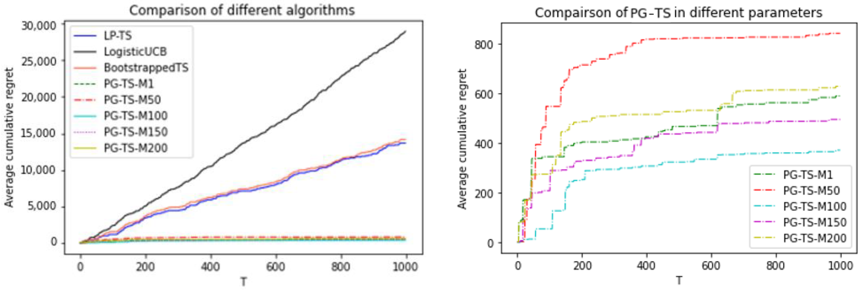
In this section, we consider two scenarios: a discrete and a continuous price experiment. To better validate the effectiveness of the proposed algorithm in this paper, in addition to the TS-LP algorithm, we also included the LogisticUCB [52] and the BootstrappedTS [53] algorithm for comparison. However, since these two algorithms are mainly applied to MAB problems with discrete action spaces, we present only the comparison results for discrete pricing experiments.

In the continuous price experiment, the feature vector of consumer $t$ is $x_t\in R^6$, where $x_{t1}=1$ denotes the intercept term. $[x_{t2},\cdots ,x_{t6}]$ are independent and identically distributed random variables obeying a Gaussian distribution with mean $[-3,-3,-3,-3,-3]$ and covariance $I_5$. We generated 1000 random data points from the above Gaussian distribution as the feature set, and we assumed that the true values of the unknown parameter $\theta$ were $[1.311,0.715,-1.545,-0.008,0.621,0.720,0.266,0.109,0.004,$$-0.175,0.433]$. The range of the price was from 0 to 300.

In the discrete price experiment, we assumed that $[x_{t2},\cdots ,x_{t6}]$, obeying a Gaussian distribution with mean $[0,0,0,0,0]$ and variance $0.25I_5$. Similarly, we generated 1000 pieces of random data obeying the above Gaussian distribution. The true values of the unknown parameter $\mathit{\theta }$ were $[0.833,0.196,0.356,-2.343,-1.085,0.560,0.939,-0.978,0.503,$$0.406,0.323]$. The set of feasible prices was $[20,40,60,80,100]$.

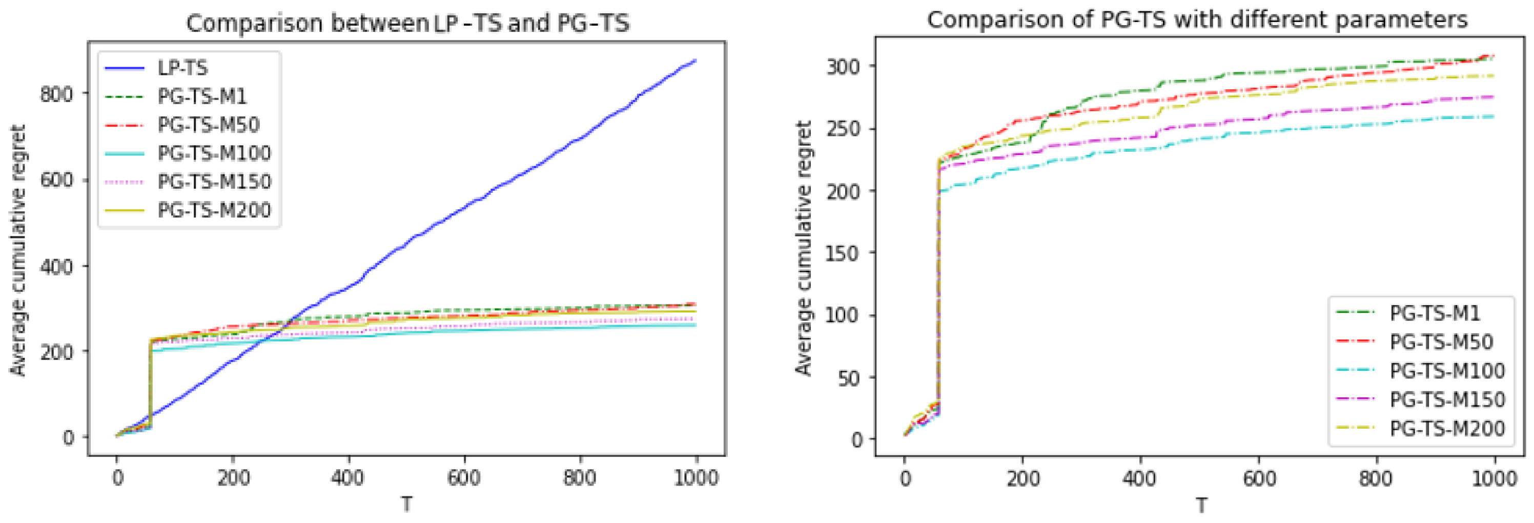
To test the performance of the PG-TS algorithm under different PG sampling parameters (i.e., M), we selected five different values of M, which were [1,50,100,150,200]. Figure 1 and Figure 2 show the results of the numerical experiments.

The figures show that in both the discrete price experiment and the continuous price experiment, the cumulative regret values of the PG-TS algorithm that we proposed were significantly lower than those of the LP-TS, LogisticUCB, and BootstrappedTS algorithms. Moreover, it can achieve convergence in a shorter period. Even when the worst M value was selected, PG-TS could converge quickly, and the cumulative regret values were much lower than those of the LP-TS algorithm. LP struggles to converge to the global optimum of the logistic likelihood function; thus, the LP-TS algorithm failed to reach convergence in both the discrete price experiment and the continuous price experiment. In addition, the convergence speed and regret value of the TS-PG algorithm did not differ much for different values of M. This shows that the performance of the algorithm proposed here is more stable.

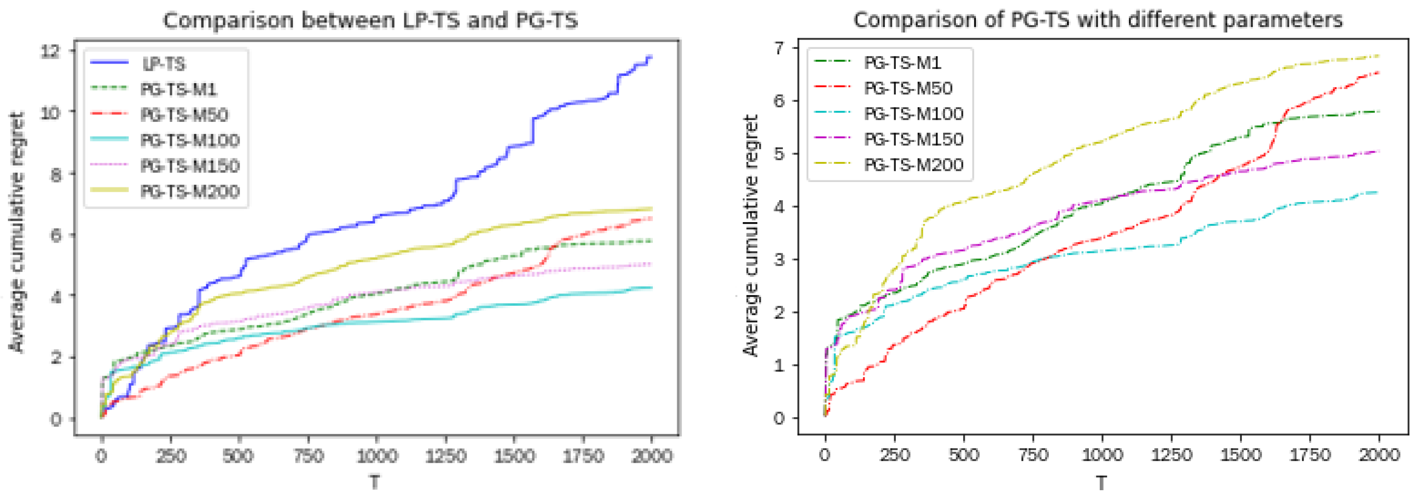
5.2. Real Experiment

In this experiment, we used an online loan dataset (i.e., CPRM-12-001: On-Line Auto Lending) provided by the Center for Revenue Management and Pricing at Columbia University’s Graduate School of Business to test the constructed algorithm. This dataset is widely used in dynamic pricing studies [48,54]. This dataset comprises 208,085 automobile loan applications received by an online lending company in the United States, spanning from July 2002 to November 2004. Each record includes the loan type applied for and the borrower’s personal information, such as loan amount, borrower’s credit score, Prime Rate, state of residence, and competitor interest rates, among other information. The online lending company determines an interest rate quote based on the borrower’s application information. Upon receiving the quote, the borrower decides whether to accept or reject it. The dataset includes the interest rate offered by the lending company for each borrower and the borrower’s decision (i.e., accept or reject).

To correspond with the personalized dynamic pricing problem described in this study, we represented the price as the net present value of the repayments. Specifically, the price was a function of the monthly repayment amount, interest rate, and loan period, which was expressed as

$$p=MonthlyPayment\times {\displaystyle \sum _{i=1}^{Term}{(1+rate)}^{-i}-LoanAmount}$$

(12)

For the sake of computational convenience, we selected the first 2000 records from the new car loan data in California, with a loan term of 36 months. In determining the feature vector, we followed the method proposed by Ban and Keskin [48]. This involves adding an intercept term to the feature data, standardizing the data, and then using a logistic regression model for feature selection. The model’s regression coefficients were considered the true values for the parameter $\theta$. Notably, using estimated parameters as true values may introduce some noise. However, the main purpose of this study was to validate the constructed algorithm in solving real problems; therefore, the above treatment is acceptable. The final element of the features includes the borrower’s credit score (FICO score), loan amount, loan prime rate, and competitor’s interest rate, with $\theta$ values being $[-2.914,0.918,0.584,1.837,-0.691,3.719,-0.116,4.546,0.356]$. Similarly to the simulated experiment, we selected five different values for M. Figure 3 shows the experimental results.

Figure 3 indicates that in the real dataset, the PG-TS algorithm demonstrates significant advantages over the LP-TS algorithm, both in terms of cumulative regret and convergence speed. When M = 100, the performance of the PG-TS algorithm is optimal. Moreover, regardless of the value of M, the regret values of the PG-TS algorithm consistently remain lower than those of the LP-TS algorithm.

5.3. Managerial Insights

In this section, we discuss the managerial insights that the findings of our study may have, aiming to assist firms in better operation and management practices.

Association between Consumer Features and Demand. Our research suggests a close association between consumers’ personalized features and product demands. Therefore, it is imperative for firms to diligently collect and analyze consumers’ personalized characteristic information, incorporating it into their pricing decision-making considerations. It is crucial to note that while collecting data, businesses must strictly adhere to data privacy and compliance regulations to protect consumers’ privacy rights and personal information security.

Data-Driven Decision Making. In practical operations, firms should utilize algorithms to analyze and process data, enabling them to more scientifically and effectively formulate pricing policies based on the analysis results. This approach helps in reducing decision-making risks and uncertainties. Furthermore, algorithmic pricing offers the advantage of real-time price adjustments, effectively addressing market changes.

Establishing Personalized Marketing Strategies. Personalized marketing not only meets the diverse needs of different consumers, enhancing consumer satisfaction, but also enables firms to generate more revenue, achieving a win–win situation for both the enterprise and consumers. To address the issue of consumers’ low acceptance of direct personalized pricing, firms can adopt indirect personalized pricing methods, such as personalized promotions. For instance, offering coupons of different denominations to different consumers and providing subsidies based on individual consumer features.

6. Conclusions

In both the corporate and academic realms, personalized dynamic pricing has had a profound impact. The judicious application of personalized pricing strategies not only increases corporate profits, but also enhances social welfare and improves consumer satisfaction. This article details the construction of a logit demand model to study personalized dynamic pricing strategies for individual consumers. We proposed a Thompson sampling algorithm based on the Polya-Gamma distribution to address the demand learning challenge in personalized pricing. Specifically, this study employed this algorithm to learn unknown parameters in the personalized demand model, establishing a Bayesian framework based on the PG distribution and providing an effective method for estimating the posterior distribution of the logistic model after parameter estimation.

Compared to the more popular methods such as LogisticUCB, BootstrappedTS, and the traditional Laplace approximation method, the PG-TS algorithm proposed in this paper performs well in balancing exploration and exploitation. However, it also has some limitations. Firstly, there are still challenges in terms of computational complexity. As the dimensionality of the feature vector increases and the PG sampling parameter M grows larger, the required computational time significantly increases. Secondly, the proposed algorithm is dependent on the prior distribution of parameters, and appropriate prior distributions contribute to better results. Thirdly, it lacks some degree of generalization ability. When faced with multinomial logistic demand models for multiple products, the proposed algorithm appears to be somewhat inadequate.

This study suggests several avenues for future research. First, the assumption of known prior distributions for unknown parameters may not hold in practice; future research could explore effective ways to learn demand in personalized pricing scenarios when the prior distribution is unknown or misspecified. Second, we did not consider differences in fairness perception among consumers resulting from personalized pricing and the consequent changes in demand. Future research could incorporate consumer fairness perception factors into the demand model, developing personalized pricing models and learning algorithms that consider the impact of consumer fairness perception. Additionally, in the real world, companies often operate in competitive environments, and future research could explore the personalized dynamic pricing issues for firms in competitive markets. Finally, future research could extend to multi-product category optimization, where consumer demand is influenced not only by prices and individual characteristics, but also by interchangeable product features.