A Multi-Step Model for Pie Cutting with Random Offers

Abstract

The problem of dividing a pie between two persons is considered. An arbitration procedure for dividing the pie is proposed, in which the arbitrator is a random number generator. In this procedure, the arbitrator makes an offer to the players at each step, and the players can either accept or reject the arbitrator’s offer. If there is no consensus, negotiations move on to the next step. At the same time, the arbitrator punishes the rejecting player by reducing the amount of the resource in favor of the consenting player. A subgame perfect equilibrium is found in the process.

1. Introduction

A classic problem in negotiation theory is the problem of fair resource sharing, which is called the pie cutting or the pie sharing problem. The pie sharing problem is relevant to various situations, such as splitting rent among housemates, resolving disputes over land ownership, and allocating work among co-workers. There is a multitude of books [1,2] and surveys [3,4,5] dealing with this topic. The situation involves representing a pie as an interval $[0,1]$, with each of the n agents possessing a value function over the pie. The main aim of the pie-sharing procedure is to divide the pie fairly. The key factors in fairly dividing a pie, as discussed in the literature, are envy-freeness and proportionality. An envy-free allocation ensures that each participant views their share as equal to or better than others’. Meanwhile, a proportional allocation guarantees that each participant receives at least $1/n$ of the value they place on the pie.

One of the popular approaches to the pie sharing problem is the Rubinstein sequential bargaining game approach [6]. In this approach, it is assumed that the players take turns suggesting to each other ways to divide a unit size pie, and the process ends as soon as all the players accept some kind of offer. Players can endlessly insist on a solution that is beneficial to themselves. To prevent this from happening, a discounting factor $\delta <1$ is introduced, i.e., the pie size at the first step is one; at the second step, it is $\delta <1$; at the third step, ${\delta }^2$, etc. A subgame perfect equilibrium is chosen as the solution to this game using the backward induction method.

Subsequently, this model was supplemented and improved. In [7], the authors built a model of multilateral negotiations with a majority rule. There, they demonstrated that a subgame perfect equilibrium exists in a discounted model in the class of stationary strategies. In this case, the player’s choices are made with equal probabilities.

In [8], a model was proposed in which the players making offers were selected with different probabilities, as well as with different discount coefficients. The uniqueness of the subgame perfect equilibrium in a game with a linear utility functions was proved.

In [9], the resource-sharing game was expanded to quadratic utility functions. A multidimensional model of sequential bargaining was presented in [10]. The asymptotic uniqueness of the equilibrium was proved in [11].

The final decision in bargaining is not necessarily made by the majority rule. The paper [12,13] examines a model of pie sharing by generating a random offer and accepting the offer through consensus. In [14,15], optimal strategies are considered in the tender competition model, and consensus models are explored in [16,17,18].

A general approach to constructing game-theoretic problems using the theory of mechanism design and the theory of active systems is examined in [19,20].

In [21,22], Rubinstein’s scheme is used to solve the problem of negotiating the time and venue of the meeting. For the general case, the existence and uniqueness of the subgame perfect equilibrium in the model with unimodal functions is proved. In [23,24], the equilibrium was found explicitly.

Depending on the scope of the model, utility functions can take an arbitrary form. For example, in [25], the problem of water resource allocation is considered using a utility function of the form $u_j\left(x\right)={\displaystyle \sum _{i=1}^k}{\beta }_i^j{u}_i\left(x_i\right)$, where $u_i\left(x\right)$ are increasing concave functions.

In this paper, we propose a multi-step pie-sharing procedure for two persons, in which the arbitrator makes offers to the players, and the players can agree with this offer or reject it. If there is no consensus, negotiations move on to the next step. The arbitrator, on the other hand, punishes the rejecting player by reducing the amount of the resource in favor of the consenting player. A subgame perfect equilibrium exists in this case.

The article is organized as follows. In Section 2, we describe the classic pie sharing problem using utility functions, which are the sizes of a player’s piece of the pie that are discounted over time. Section 3 presents a new design in the pie-sharing procedure, in which, when a player is punished, their share is changed in favor of the other player. In Section 4, a class of threshold strategies is introduced, and the equilibrium in this game is found in the class of threshold strategies. Section 5 suggests a matrix method for determining the type of optimal strategies at each step. Section 6 relates the results of the computer simulation of the pie division in the case where one of the players uses an equilibrium strategy and the other player deviates from the equilibrium strategy.

2. Two-Person Cake-Cutting Problem

Let us consider the problem of dividing a unit-size pie between two persons. We assume that a sequential bargaining design is used for the solution [1]. With this approach, the players take turns suggesting to each other ways to divide a unit-size pie and the process ends once one of them accepts the other’s offer. For the sake of certainty, let the first player make the offer at the first step and at further odd steps, and the second player at even steps. At each step, the resource is discounted and the discounting factor is $\delta <1$.

To find a solution, we introduce the utility functions of the players, i.e., if bargaining results in a decision $x\in [0,1]$, then the players get utilities expressed by the functions $u_1\left(x\right)=x,x\in [0,1]$ and $u_2\left(x\right)=1-x,x\in [0,1]$, respectively. We assume that the players take turns offering solutions and the consent of both participants is required to make the decision. At the same time, the utilities get discounted over time, i.e., after each bargaining session, the utility functions of both players will decrease proportionally to $\delta$. Thus, if the players have not come to a decision before time t, then at time t, their utilities are represented by functions ${\delta }^{t-1}{u}_i\left(x\right),i=1,2$.

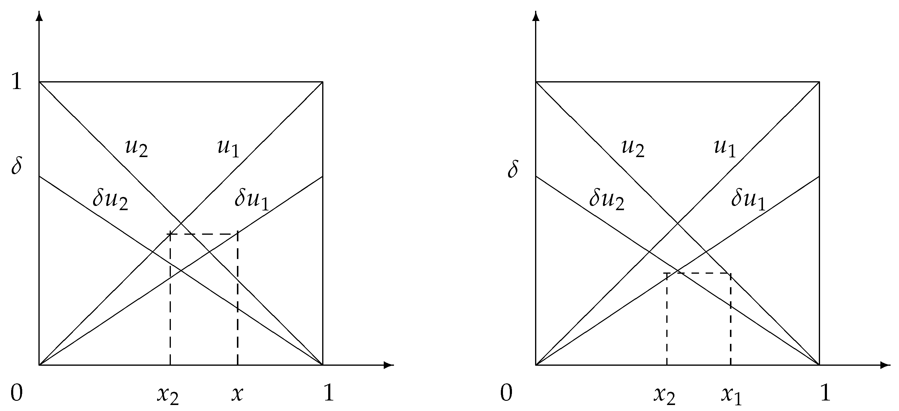
In this case, the problem is equivalent to the problem of sharing the pie between two persons. Indeed, if x is construed as a share of the pie, then the second participant gets the rest of the pie $1-x$. Figure 1 shows utility graphs of $u_1\left(x\right)$ and $u_2\left(x\right)$ and their graphs in the next step, i.e., $\delta u_1\left(x\right)$ and $\delta u_2\left(x\right)$.

Let us assume that player 2 knows the solution x that player 1 will choose in the next step. To ensure that a decision is made, she/he needs to offer the first player a solution y such that their utility $u_1\left(y\right)$ is not less than the utility in the next step, i.e., $\delta u_1\left(x\right)$ (see Figure 1). This leads to the inequality $y\ge \delta x$, and the utility of player 2 herself/himself is maximized at $y=\delta x$. Thus, her/his optimal response to the first player’s strategy x will be $x_2=\delta x$. Next, we assume that the first player knows the second player’s strategy $x_2$ in the next step. Then, in order for her/his offer at this step to be accepted by player 2, she/he must propose a solution y such that the utility of the second player $u_2\left(y\right)$ is not less than her/his utility at the next step, i.e., $\delta u_2\left(x_2\right)$, which is equivalent to the inequality $1-y\ge \delta (1-\delta x)$ or $y\le 1-\delta (1-\delta x)$.

It follows that the best response of the first player at this step is $x_1=1-\delta (1-\delta x)$. The solution x produces an equilibrium in the bargaining if $x_1=x$ or $x=1-\delta (1-\delta x)$, wherefore

$$x^{*}=\frac{1}{1+\delta },$$

which coincides with the classical solution.

3. Bargaining over a Time-Varying Resource

This paper proposes a new bargaining design for the pie sharing problem. There are still two players who want to divide a unit-size pie between themselves, but now an arbitrator is introduced into the game. The bargaining solution is $x\in [0,1]$. The utility functions of players 1 and 2 are equal, respectively, to the following:

$$\left\{\begin{array}{cc}{u}_1\left(x\right)=x\hfill & x\in [0,1],\hfill \\ u_2\left(x\right)=1-x\hfill & x\in [0,1].\hfill \end{array}\right.$$

Utility functions will not change under this approach. Instead, the resource itself will change.

Negotiations are sequential in time. At each step, the arbitrator makes an offer to the players. Her/his offer at step t ${\alpha }_t$ is modeled by a random variable having a uniform distribution on the unit interval ${\alpha }_t\in [0,1]$. The players, on the other hand, agree to this offer (action A) or reject it (action R). If both players agree at step t, the game ends and the players get payoffs of

$$\left\{\begin{array}{c}{u}_1={\alpha }_t,\hfill \\ u_2=1-{\alpha }_t.\hfill \end{array}\right.$$

If at least one of the players rejects the offer, the game moves on to the next step, and the interval is reduced by $\delta$ times, the penalty being imposed on the rejecting player. Here, $\delta <1$ is the discount factor.

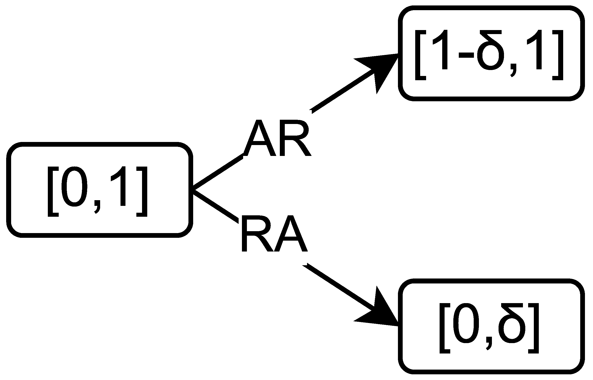
The punishment is carried out as follows (see Figure 2). If the first player refuses (situation ($R,A$)), the initial interval $[0,1]$ is changed in the next step to the interval $[0,\delta ]$. Thus, the maximum utility of player 1 becomes smaller. If the second player refuses (the situation ($A,R$)), the initial interval $[0,1]$ is changed to the interval $[1-\delta ,1]$, i.e., the maximum utility of player 2 becomes smaller.

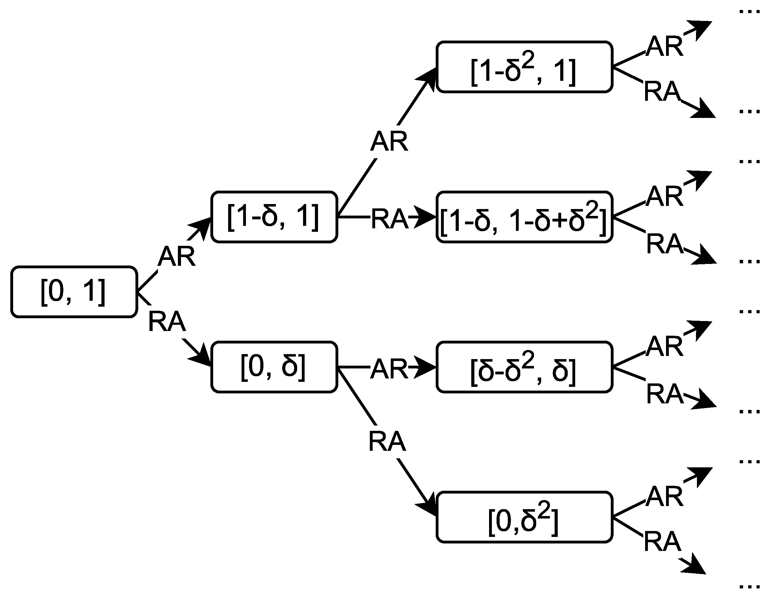
At subsequent steps, the situation recurs (see Figure 3), where, at step t, the interval for the offers has the form $[a_t,b_t]$. If the first player rejects the offer at step $t+1$, the interval $[a_t,b_t]$ takes the form $[a_t,a_t(1-\delta )+b_t\delta ]$. If the second player refuses, the interval $[a_t,b_t]$ takes the form $[a_t\delta +b_t(1-\delta ),b_t]$.

In the situation $(R,R)$, when both players refuse, we suppose that the players are penalized equally, and the interval $[a_t,b_t]$ becomes $[(a_t+b_t)/2-\delta /2,(a_t+b_t)/2+\delta /2]$.

For clarity, we substitute $\delta =0.9$. Large values of $\delta$ show that players are patient and are willing to play the game for a long time. If the first player refuses, the interval becomes $[0,0.9]$. If the second player refuses, then the interval at the second move becomes $[0.1,1]$.

Let us now substitute $\delta =0.1$. Small values indicate that the players are impatient and wish to finish the game as quickly as possible. If the first player refuses, the interval becomes $[0,0.1]$. If the second player refuses, the interval at the second move is $[0.9,1]$.

Each of the players is interested in maximizing their utility function. Based on the form of these functions, the first player wants to settle on an offer close to 1, and the second player would like to settle on an offer close to 0. The interval for the offers changes over time, so the players’ strategies must be time-dependent. Let us denote the players’ strategies as $\{S_t^1,S_t^2\},t=1,2,\dots$. The equilibrium strategies of the players $\{S_t^{1*},S_t^{2*}\},t=1,2,\dots$ are defined by the conditions

$$u_1\left(S_t^1,S_t^{2*}\right)\le u_1\left(S_t^{1*},S_t^{2*}\right),u_2\left(S_t^{1*},S_t^2\right)\le u_2\left(S_t^{1*},S_t^{2*}\right), \forall S_t^{1*},S_t^{2*},t=1,2,\dots$$

4. Threshold Strategies

We look for a solution in the class of threshold strategies of the following form:

$$S^1=\left\{\begin{array}{c}\hfill A,\mathrm{if}\alpha \ge s_1,\hfill \\ \hfill R,\mathrm{if}\alpha <s_1,\hfill \end{array}\right. S^2=\left\{\begin{array}{c}\hfill A,\mathrm{if}\alpha \le s_2,\hfill \\ \hfill R,\mathrm{if}\alpha >s_2.\hfill \end{array}\right.$$

For the first player, the strategy is determined by a threshold $s^1\in [0,1]$. If the referee’s offer is $\alpha \ge s^1$, the first player accepts the offer; otherwise, she/he rejects it.

The second player’s strategy is determined by the threshold $s^2\in [0,1]$. The second player accepts the arbitrator’s offer if $\alpha \le s^2$ and rejects is otherwise. Let us assume $s^1\le s^2$. This assumption can be made without any loss of generality; if we suppose $s^1>s^2$, then the second player could change their strategy by adjusting the threshold to $s^1$. Depending on the step number t, we denote the strategy profile by $\{s_t^1,s_t^2\},t=1,2,3,\dots$. These numbers indicate the extreme values that players will agree on.

The recurrence relations for the thresholds depending on the step number are as follows. Suppose at step t of the game the negotiation interval is $[a_t,b_t]$. At the next step, depending on the players’ decision, the negotiation interval will change.

If the situation $(A,R)$ occurs, then the boundaries of the interval at the next step can be found by the formula

$$\left\{\begin{array}{c}{a}_{t+1}=a_t\delta +b_t(1-\delta ),\hfill \\ b_{t+1}=b_t.\hfill \end{array}\right.$$

(1)

If the players’ solution is $(R,A)$, then the boundaries are found by the formula

$$\left\{\begin{array}{c}{a}_{t+1}=a_t,\hfill \\ \hfill b_{t+1}=a_t(1-\delta )+b_t\delta .\hfill \end{array}\right.$$

(2)

In the matrix form, relations (1) and (2) can be written, respectively, as

$$(a_{t+1},b_{t+1})=(a_t,b_t)\left(AR\right),(a_{t+1},b_{t+1})=(a_t,b_t)\left(RA\right),$$

where the matrices $\left(AR\right)$ and $\left(RA\right)$ have the form

$$\left(AR\right)=\left(\begin{array}{cc}\delta & 0\\ 1-\delta & 1\end{array}\right),\left(RA\right)=\left(\begin{array}{cc}1& 1-\delta \\ 0& \delta \end{array}\right).$$

(3)

Lemma 1.

At step n, if the history of the game is

$${(A,R)}^{i_1},{(R,A)}^{i_2},\cdots ,{(A,R)}^{i_k},$$

where $i_1+i_2+\cdots +i_k=n$, $i_j⩾0,j=1,\dots k,$ then the boundaries of the negotiation interval can be expressed as

$$(a_n,b_n)=(0,1)·{\left(AR\right)}^{i_1}·{\left(RA\right)}^{i_2}·\cdots ·{\left(AR\right)}^{i_k},$$

where the matrices $\left(AR\right)$ and $\left(RA\right)$ have the form (3).

Seeking to find the optimal behavior of the players, we use mathematical induction. Suppose that at step n the players decided to end the game and accept the arbitrator’s offer. If the interval for negotiation was $[a_n,b_n]$, then the average value for the first player’s chosen offer will be $H_n=(a_n+b_n)/2$.

Let us find the optimal strategies of the players at the previous step $n-1$. Suppose that at this step the negotiation interval is $[a_{n-1},b_{n-1}]$, and let the players choose the threshold strategies with thresholds $s^1,s^2$. Then, the first player’s payoff is

$$\begin{array}{c}{H}_{n-1}(s^1,s^2)=\frac{1}{b_{n-1}-a_{n-1}}\left(\underset{a_{n-1}}{\overset{s^1}{\int }}\frac{2a_{n-1}+\delta (b_{n-1}-a_{n-1})}{2}da+\right.\\ \left.+\underset{s^1}{\overset{s^2}{\int }}ada+\underset{s^2}{\overset{b_{n-1}}{\int }}\frac{2b_{n-1}-\delta (b_{n-1}-a_{n-1})}{2}da\right)=\\ =\frac{1}{b_{n-1}-a_{n-1}}\left(\frac{{\left(s^2\right)}^2-{\left(s^1\right)}^2}{2}+(s^1-a_{n-1})\frac{2a_{n-1}+\delta (b_{n-1}-a_{n-1})}{2}\right.+\\ \left.+(b_{n-1}-s^2)\frac{2b_{n-1}-\delta (b_{n-1}-a_{n-1})}{2}\right)\end{array}$$

(4)

The saddle point of function (4) has the form

$$s^{1*}=a_{n-1}+\frac{\delta (b_{n-1}-a_{n-1})}{2},s^{2*}=b_{n-1}-\frac{\delta (b_{n-1}-a_{n-1})}{2}.$$

Substituting it into the payoff function (4), we obtain

$$H_{n-1}(s^{1*},s^{2*})=\frac{a_{n-1}+b_{n-1}}{2}.$$

Thus, under optimal behavior, the payoff at each step t represents the midpoint of the interval $[a_t,b_t]$. Applying induction, we obtain the following proposition.

Proposition 1.

A subgame perfect equilibrium in a negotiation game with a time-varying resource has the following form:

$$S_t^1=\left\{\begin{array}{c}\hfill A,if{\alpha }_t\ge s_t^1,\hfill \\ \hfill R,if{\alpha }_t<s_t^1,\hfill \end{array}\right. S_t^2=\left\{\begin{array}{c}\hfill A,if{\alpha }_t\le s_t^2,\hfill \\ \hfill R,if{\alpha }_t>s_t^2.\hfill \end{array}\right.$$

where thresholds $s_t^1,s_t^2$ are defined by the relations

$$s_t^{1*}=a_t+\frac{\delta (b_t-a_t)}{2},s_t^{2*}=b_t-\frac{\delta (b_t-a_t)}{2}.$$

(5)

Note that according to (5), the length of the interval $[s_t^1,s_t^2]$ at step t is equal to

$$s_t^{2*}-s_t^{1*}=(b_t-a_t)(1-\delta ).$$

If the arbitrator’s offer falls within this interval, the players stop playing. The probability of this event is $1-\delta$. This event recurs at each negotiation step. Thus, the probability of taking a final decision within finite time under optimal behavior

$$(1-\delta )+\delta (1-\delta )+{\delta }^2(1-\delta )+\dots$$

equals 1.

Remark 1.

According to (5), the optimal strategies in the first step are of the form $s_1^{1*}=\delta /2, s_1^{2*}=1-\delta /2$. If the arbitrator’s offer is $\alpha \le \delta /2$, the second player accepts the offer while the first player rejects it. In this case, the game moves on the next step, player 1 is penalized, and the negotiation interval becomes $[0,\delta ]$.

If the arbitrator’s offer is $\alpha \ge 1-\delta /2$, the first player accepts the offer, while the second player rejects it. In this case, the game moves on to the next step, but now player 2 is penalized and the negotiation interval becomes $[1-\delta ,1]$.

If the arbitrator’s offer falls within the interval $[\delta /2,1-\delta /2]$, the negotiation ends, and the players accept the offer.

5. Optimal Strategies

According to Lemma 1, if the history of the game has the form

$${(A,R)}^{i_1}\cdots ,{(R,A)}^{i_k},$$

where $i_1+\cdots +i_k=n$, $i_j⩾0,j=1,\cdots k,$ then the boundaries of the negotiation interval at step n are calculated by the formula

$$(a_n,b_n)=(0,1)·{\left(AR\right)}^{i_1}\cdots {\left(RA\right)}^{i_k}.$$

(6)

In this case, some of the powers of $i_j$ may be zero. Note that the eigenvalues of the matrices $\left(AR\right)$ and $\left(RA\right)$ are equal to 1 and $\delta$. In this case, these matrices can be represented in the form

$$\left(AR\right)=T_1\Lambda T_1^{-1},\left(RA\right)=T_2\Lambda T_2,$$

where

$$T_1=\left(\begin{array}{cc}0& 1\\ 1& -1\end{array}\right),T_1^{-1}=\left(\begin{array}{cc}1& 1\\ 1& 0\end{array}\right),T_2=T_2^{-1}=\left(\begin{array}{cc}1& 1\\ 0& -1\end{array}\right),\Lambda =\left(\begin{array}{cc}1& 0\\ 0& \delta \end{array}\right).$$

Then, (6) can be rewritten in the form

$$(a_n,b_n)=(0,1)·T_1{\Lambda }^{i_1}{T}_1^{-1}\cdots T_2{\Lambda }^{i_k}{T}_2.$$

Denoting

$$T_3=T_1^{-1}{T}_2=\left(\begin{array}{cc}1& 0\\ 1& 1\end{array}\right)$$

and noticing that $T_2{T}_1=T_3^{-1}$, we find the boundaries of the negotiation interval at step n for history

$$(a_n,b_n)=(0,1)·T_1{\Lambda }^{i_1}{T}_3{\Lambda }^{i_2}{T}_3^{-1}\cdots {\Lambda }^{i_k}{T}_2.$$

(7)

It follows from statement 1 that the thresholds for optimal strategies at step n in matrix form have the form

$$(s_n^1,s_n^2)=(a_n,b_n)·D=(a_n,b_n)\left(\begin{array}{cc}1-\frac{\delta }{2}& \frac{\delta }{2}\\ \frac{\delta }{2}& 1-\frac{\delta }{2}\end{array}\right).$$

Proposition 2.

At the n-th step of the game, when the negotiation history has the form

$${(A,R)}^{i_1}\cdots ,{(R,A)}^{i_k},$$

where $i_1+\cdots +i_k=n$, $i_j⩾0,j=1,\cdots k,$ the thresholds of equilibrium strategies have the form

$$(s_n^{*1},s_n^{2*})=(0,1)·T_1{\Lambda }^{i_1}{T}_3{\Lambda }^{i_2}{T}_3^{-1}\cdots {\Lambda }^{i_k}{T}_2·D,$$

where the matrix D has the form

$$D=\left(\begin{array}{cc}1-\frac{\delta }{2}& \frac{\delta }{2}\\ \frac{\delta }{2}& 1-\frac{\delta }{2}\end{array}\right).$$

For example, if during the bargaining process the situation $(A,R)$ occurred twice, the situation $(R,A)$ three times, and then again the situation $(A,R)$ two times, then the boundaries of the negotiation interval at step 7 have the following form:

$$(a_7,b_7)=(0,1)·T_1{\Lambda }^2{T}_3{\Lambda }^3{T}_3^{-1}{\Lambda }^2{T}_1^{-1}=$$

$$(0,1)\left(\begin{array}{cc}0& 1\\ 1& -1\end{array}\right)\left(\begin{array}{cc}1& 0\\ 0& {\delta }^2\end{array}\right)\left(\begin{array}{cc}1& 0\\ 1& 1\end{array}\right)\left(\begin{array}{cc}1& 0\\ 0& {\delta }^3\end{array}\right)\left(\begin{array}{cc}1& 0\\ -1& 1\end{array}\right)\left(\begin{array}{cc}1& 0\\ 0& {\delta }^2\end{array}\right)\left(\begin{array}{cc}1& 1\\ 1& 0\end{array}\right),$$

whence we get

$$a_7=1-{\delta }^2+{\delta }^5-{\delta }^7,b_7=1-{\delta }^2+{\delta }^5.$$

The optimal thresholds that players should use are found from the relations

$$(s_7^{1*},s_7^{2*})=(1-{\delta }^2+{\delta }^5-{\delta }^7,1-{\delta }^2+{\delta }^5)\left(\begin{array}{cc}1-\frac{\delta }{2}& \frac{\delta }{2}\\ \frac{\delta }{2}& 1-\frac{\delta }{2}\end{array}\right),$$

and, consequently,

$$s_7^{1*}=1-{\delta }^2+{\delta }^5-{\delta }^7(1-\frac{\delta }{2}),s_7^{2*}=1-{\delta }^2+{\delta }^5-\frac{{\delta }^8}{2}.$$

6. Numerical Simulation

Suppose that both players use optimal strategies. The number of games in the experiment is 1000. The notations are n for the average number of moves per game, $U_1$ for the average payoff of the first player, and $U_2$ for the average payoff of the second player. For both payoffs, the confidence interval with a reliability of $0.99$ is given in parentheses.

Table 1. Both players use optimal strategies.

$\mathit{\delta }$	n	${\mathit{U}}_1$	${\mathit{U}}_2$
$0.9999$	11,420.83	$0.5$, $[0.4996,0.5005]$	$0.5$, $[0.4995,0.5004]$
$0.9$	$9.29$	$0.5$, $[0.4915,0.52]$	$0.5$, $[0.4799,0.5085]$
$0.8$	$5.28$	$0.5$, $[0.4887,0.5173]$	$0.5$, $[0.4740,0.5156]$
$0.6$	$2.45$	$0.51$, $[0.4881,0.5449]$	$0.49$, $[0.4550,0.5230]$
$0.2$	$1.25$	$0.52$, $[0.482,0.5642]$	$0.48$, $[0.4628,0.5360]$

shows the numerical simulation results.

Consider the line at $\delta =0.9999$. The discount factor close to one shows the players’ willingness to bargain for a long time, and, indeed, the average number of moves in the game is 11,420.83. In this case, the payoffs of both players and the confidence intervals are close to the value $0.5$.

If, for example, $\delta =0.6$, then we observe a decrease in the average number of moves in the game to $2.45$, i.e., the players will not bargain for a long time. At the same time, for both players, the mean payoffs are $0.5$, but the confidence intervals for the mean increases. For the first player, the confidence interval widens to $[0.4881,0.5449]$, and for the second player to $[0.4550,0.5230]$.

Table 2. The second player uses a suboptimal strategy.

$\mathit{\delta }$	${\mathit{s}}_2$	n	${\mathit{U}}_1$	${\mathit{U}}_2$
$0.9999$	$0.2$	$5083.11$	$0.5026$, $[0.5023,0.5029]$	$0.4974$, $[0.4971,0.4977]$
$0.9999$	$0.4$	$2868.93$	$0.503$, $[0.5028,0.5035]$	$0.497$, $[0.496,0.497]$
$0.9999$	$0.5$	$1459.61$	$0.502$, $[0.5019,0.5023]$	$0.498$, $[0.497,0.498]$
$0.8$	$0.2$	$8.21$	$0.63$, $[0.606,0.646]$	$0.37$, $[0.354,0.394]$
$0.8$	$0.4$	$4.60$	$0.64$, $[0.612,0.653]$	$0.36$, $[0.347,0.388]$
$0.8$	$0.5$	$3.24$	$0.66$, $[0.644,0.682]$	$0.34$, $[0.318,0.356]$
$0.6$	$0.2$	$4.57$	$0.56$, $[0.531,0.581]$	$0.44$, $[0.412,0.469]$
$0.6$	$0.4$	$3.34$	$0.58$, $[0.564,0.613]$	$0.41$, $[0.387,0.436]$
$0.6$	$0.5$	$2.30$	$0.61$, $[0.584,0.643]$	$0.39$, $[0.356,0.416]$
$0.2$	$0.2$	$1.53$	$0.57$, $[0.534,0.612]$	$0.43$, $[0.388,0.467]$
$0.2$	$0.4$	$1.49$	$0.52$, $[0.479,0.563]$	$0.48$, $[0.436,0.521]$
$0.2$	$0.5$	$1.54$	$0.515$, $[0.475,0.556]$	$0.485$, $[0.444,0.525]$

shows the results of numerical simulations for the situation where the first player uses an equilibrium strategy and the second player uses a strategy with a constant threshold $s_2$ that does not change throughout the game. A column is added to the table to show the strategy of the second player in the game.

Consider the case for $\delta =0.9999$. The second player’s strategy $s_2=0.2$ indicates that the player wants to obtain a large payoff, namely, $0.8$. With such a large value of $\delta$, the game lasts, on average, $5083.11$ moves. However, we see that the second player obtains a payoff of $0.498$, while the first player obtains a larger payoff, namely, $0.502$. This shows the effectiveness of the first player’s optimal strategy. If the second player uses a less greedy strategy $s_2=0.5$, their payoff will still be less than the first player’s, namely, $0.498$.

Now, consider the case of smaller value $\delta =0.6$. When the second player uses the greedy strategy $s_2=0.2$, the average number of moves in the game is $4.57$. Note that this is almost twice as large as it is when both players use optimal strategies. However, the second player’s payoff is $0.44$, and even the right-hand boundary of the confidence interval does not go beyond $0.5$. The use of a less greedy strategy $s_2=0.5$ by the second player will only reduce their payoff from $0.44$ to $0.39$. Thus, we see that the second player’s unwillingness to use the optimal strategy can lead to a significant decrease in their payoff.

7. Conclusions

In this paper, a new design is proposed in the two-person pie sharing problem involving an arbitrator. This is a multi-step procedure, and the solution is reached by consensus. The arbitrator is represented by a random number generator, which is easy to implement in practice. The procedure is fair for both players, and both players are on equal terms. It is demonstrated that deviations from the optimal strategy lead to a decrease in payoff.

This method is described for the two-person pie sharing problem. We plan to transfer this scheme to the case of several players and other utility functions. It is also possible to apply this procedure to the problems of resource allocation and contests.