1. Introduction
Solving linear matrix equations is a very important topic in control theory. Such equations include Lyapunov equations and Sylvester equations. Let
, where
E is singular. Assume that the pencil
is d-stable. That is, the moduli of all finite eigenvalues of the pencil
are less than 1. According to [
1], there exist nonsingular
matrices
that transform
into a Weierstrass canonical form, i.e.,
with
and
. Define the left and right spectral projection matrices
,
by
In this paper, we focus on the numerical solution of the discrete-time projected Lyapunov equation
where
is the solution,
. Here and in the following, the superscript
T denotes the transpose of a vector or a matrix. Since
is d-stable, (
3) has a symmetric positive semi-definite solution; see, for example, ref. [
2]. The discrete-time Lyapunov equation is also called the Stein equation in the literature. By using the Kronecker product [
3], the first equation in (
3) can be formulated as
, where
, and
is the
i-th column of
X.
The Stein equation with nonsingular
E plays an essential role in discrete-time dynamical systems, including stability analysis and control [
4,
5,
6], model reduction [
7,
8,
9,
10,
11,
12], solutions of discrete-time algebraic Riccati equations (by Newton’s method) in optimal control [
13], and the restoration of images [
14]. In contrast, the projected Stein equation arises in the balanced truncation model reduction [
2] of discrete-time descriptor systems. In the positive real and bounded real balanced truncation model reduction of discrete-time descriptor systems, we also need to solve a projected Stein equation at each iteration step of Newton’s method for projected Riccati equations.
In the past few decades, many researchers have focused on constructing numerically robust algorithms for the standard Stein equation, i.e., with
E being the identity matrix. For example, a standard direct method was provided in [
15], which is a direct extension of the well-known Bartels–Stewart algorithm [
16] for continuous-time Lyapunov equations
to the standard Stein equation. Hammarling [
17] proposed a variant of the Bartels–Stewart algorithm for both the continuous-time and discrete-time cases. This variant is named the Hammarling method in the literature and aims to compute the Cholesky factor of the solution, which is desired in the balanced truncation model order reduction of discrete-time systems. The Hammarling algorithm was further improved in [
18,
19] by using a rank-2 updating formula. These approaches are based on the real Schur decomposition, require a computational complexity of
flops, and thus are only suitable for small to moderately sized problems.
It is known that the solution matrix of a continuous-time Lyapunov equation has a low numerical rank in cases where it has a low-rank right-hand side; see, e.g., ref. [
20]. Specifically, the low numerical rank means that the singular values of the solution
X decay very rapidly. Penzl [
21] showed theoretically that the singular values of the solution decay exponentially for the continuous-time Lyapunov equation with a symmetric coefficient matrix and a low-rank right-hand side. Baker, Embree, and Sabino [
22] considered the nonsymmetric case, and they explained that a larger departure from normality probably means a faster decay of singular values. The fact that the solution has a rapid decay of singular values and can be well approximated by its low-rank factorization now enables the use of numerous iterative methods that seek accurate low-rank approximations to the solution. These iterative methods include the low-rank Smith method [
23,
24], the Cholesky factor alternating-direction implicit (ADI) method [
25], the (generalized) matrix sign function method [
26], and the extended Krylov subspace method [
27], to name a few. For the continuous-time projected Lyapunov equation, Stykel [
28] extended the low-rank ADI method and the low-rank Smith method to compute low-rank approximations to the solution. In [
13], the ADI method was extended to discrete-time Lyapunov equations and was further improved to compute the real factors in [
29] by utilizing the technique that was proposed in [
30] for continuous-time Lyapunov equations.
In recent years, numerical methods for continuous-time Lyapunov equations have been further considered. In [
31], a class of low-rank iterative methods is proposed by using Runge–Kutta integration methods. It is shown that a special instance of this class of methods is equivalent to the low-rank ADI method. In [
32], Benner, Palitta, and Saak further improved the low-rank ADI. They used the extended Krylov subspace method to solve the shifted linear system at each iteration. It is shown that by using only a single subspace, all the shifted linear systems can be solved to achieve a prescribed accuracy. In [
33], the authors considered the inexact rational Krylov subspace method and low-rank iteration, in which a shifted linear system of equations is solved inexactly. In [
34,
35], the choice of shift parameters is considered, and some selection techniques are proposed to achieve a fast convergence for the low-rank ADI method.
In this paper, we first transform the projected generalized Stein Lyapunov Equation (
3) to an equivalent projected standard Stein equation and then extend the low-rank Smith method to the projected standard equation. After this, we extend the low-rank ADI method to (
3) and propose how to compute the real low-rank factor by following the idea in [
29,
30]. We also consider the choice of ADI shift parameters. Finally, through two standard numerical examples from discrete-time descriptor systems, we show the efficiency of the proposed low-rank ADI method.
The main contributions of this paper include the following:
The low-rank ADI method is extended to solve the discrete-time projected Lyapunov equation.
A partially real low-rank ADI algorithm is proposed.
Two numerical examples are presented to demonstrate the good convergence of the low-rank ADI method.
The low-rank ADI method is one of the most commonly used iterative methods for solving linear matrix equations. It has a good convergence curve, although the shift parameters are not optimal. Moreover, it always produces a low-rank positive semi-definite approximate solution for Lyapunov equations, which is desired for some applications, such as the balanced truncation model order reduction. In contrast, the Krylov subspace method cannot guarantee the generation of the positive semi-definite solution. The main drawback of the low-rank ADI method is that it requires selecting shifts and solving one linear system of equations for each iteration.
The rest of the paper proceeds as follows. In
Section 2, we reformulate (
3) and propose the low-rank Smith method. In
Section 3, we extend the real version of the low-rank ADI method for the projected Stein equation.
Section 4 is devoted to two numerical examples. Finally, conclusions are given in
Section 5.
2. Low-Rank Smith Method
The Smith method [
36] was originally proposed for solving the continuous-time Sylvester equation
. First, the continuous-time equation is equivalently transformed to a discrete-time equation via a Cayley transform. Then, the Smith iteration is derived from the series representation of the solution. For the projected Stein Equation (
3), the Smith method can be applied directly without the Cayley transform.
Due to the singularity of
E, its inverse does not exist. We use the
-inverse
of
E, which is defined by
see, e.g., ref. [
37]. For the generalized inverse of a singular matrix, the interested reader is referred to [
38].
Multiplying the first equation in (
3) from the left and right by
and
and using
,
, and
, we obtain
The unique solution of (
4) can be formulated as
Since the pencil
is d-stable, the spectrum radius
of
, which is defined by
, satisfies
. So, the series converges, and the solution
X is symmetric positive semi-definite, i.e.,
. This series representation of the solution implies that the numerical rank of
X is much smaller than its dimension
n if the norm of the powers of
decreases rapidly. In [
39], Benner, Khoury, and Sadkane considered the solution of the Stein equation with
and obtained an inequality that explicitly describes the decay of the singular values of the solution. For the projected Stein Equation (
4), by following [
39], we can obtain
where
denote the singular values of the solution
X. This result explicitly shows that the solution has a low numerical rank if the norm of the powers of
decreases rapidly.
We can now apply the Smith method [
24,
28] to (
4). It is a fixed-point iteration and is expressed as
This iteration converges since
, and the iterations can be written as the partial sum
We see from (
6) that the iterations can be reformulated by a low-rank representation of Cholesky factors, i.e.,
with
. It follows from (
5) and (
6) that the error matrix
can be expressed as
Consequently, we can obtain the relative error bound
This shows that converges linearly to the solution if the spectrum radius , and X can be accurately approximately by the low-rank iteration if the norm of the powers of decreases rapidly. Note that the norm of the error matrix is not computable since the solution X is unknown. For large-scale problems, it is also difficult to accurately estimate the relative error bound .
For the residual matrix
defined by
we have
So, the Frobenius matrix norm of
can be easily computed.
The dimension of the low-rank factor
will increase by
m in each iteration step. Hence, if the Smith iteration converges slowly, the number of columns of
will easily reach unmanageable levels of memory requirements. To reduce the dimension of
, we will approximate it by using the rank-revealing QR decomposition (RRQR) [
40]. Assume that
has the low numerical rank
with a prescribed tolerance
. Consider the RRQR decomposition of
with column pivoting:
where
is an upper triangular matrix with
and
,
is orthogonal,
is a permutation matrix, and
has
columns. Then,
can be approximated by
where
The low-rank Smith method for solving the projected Stein Equation (
3) is presented in Algorithm 1.
| Algorithm 1 Low-rank Smith method |
- Input:
, , . - Output:
Z such that is the approximate solution of ( 3)
Set , , ; Compute the rank-revealing QR decomposition
While do
- •
. - •
. - •
. - •
Compute the rank-revealing QR decomposition
- •
End While |
The main advantage of the Smith iteration (
6) is that it is very simple and can be easily implemented. However, we should note that the iterations converge very slowly if the spectrum radius
. This is a significant motivation for further improvement of the Smith method.
3. Low-Rank ADI Method
The ADI method was first introduced in [
41] and then applied to solve continuous-time Lyapunov matrix equations in [
42]. Recently, this method was extended to the Stein Equation (
3) by Benner and Faßbender [
13] and further improved in [
29]; see also [
43].
For the projected Stein Equation (
3), by generalizing the ADI method, we iteratively compute approximations
,
, of the solution
X by following the iteration scheme
where
denotes suitable shift parameters. Note that, although the iteration can work with any initial guess
, we use only
in the sequel.
Since the pencil
is d-stable and
, the matrices
and
are nonsingular. From (
8), we obtain
Then, these half steps in the ADI iteration are rewritten into single steps by substituting
into (9) by the expression (
10) for
; i.e., we arrive at the single-step iteration
Observe that
Hence, we obtain
Multiplying (
13) from the left by
and using
,
for any
, we obtain
One can easily verify that the solution
X of the projected Stein Equation (
3) is a fixed point of the single-step iteration (
14). That is to say,
Consequently, from (
14) and (
15), we obtain the following recursive formulation for the error matrix between the solution
X and the approximation
:
We see from (
16) and
that the error matrix
can be written as
3.1. Low-Rank Version of ADI Method
For continuous-time Lyapunov equations with a low-rank right-hand side, Li and White [
25] proposed the state-of-the-art Cholesky factor ADI algorithm, which generates a low-rank approximation to the solution. This method is a significant improvement of the ADI method [
42] and is very appropriate for large-scale continuous-time Lyapunov equations. The Cholesky factor ADI method is developed by exploiting the low-rank structure of the iterations and reordering the shifts; see [
25] for the details. The low-rank ADI method is generalized to the Stein equation in [
29].
In this section, we follow these ideas to deduce the low-rank ADI method for the projected Stein Equation (
3). Suppose now that
and
are written in their factored forms:
and
. Then, from (
14), we obtain the following recursive relation for
and
:
with
.
From (
18), we easily see that the dimension of
would increase by
m at each iteration step. Therefore, the factor
of
has
columns. Since the number of columns increases by
m at each iteration, the number of systems of linear equations with matrices
, which need to be solved at each iteration in the low-rank ADI method (
18), increases by
m. So, this iteration (
18) for the factors is not suitable for practical implementation. By making use of the trick in [
25],
can be reformulated as
where
This directly leads to an efficient low-rank ADI iteration scheme: Let
, and
. Then, for
,
We now investigate the residual matrix corresponding to the j-th approximate solution . In the following theorem, we show that has a low-rank factorization of rank at most m.
Theorem 1. Let , where is the j-th iteration generated by the low-rank ADI for the projected Stein Equation (3), and let the matrix be defined by (19). Then, the residual matrix , defined by (7), can be formulated as Proof. From (
3),
. Thus,
By inserting (
17) into (
22), we obtain
From (
19) and (20), and
, it follows that
Thus,
. □
The following theorem states that and can be obtained without solving systems of linear equations once has been computed.
Theorem 2. Assume that a proper set of shift parameters is used in the low-rank ADI iteration. For the two subsequent blocks and related to the pair of complex shifts with , it holds thatMoreover, after applying a pair of complex shifts , the generated is real. Proof. Although the proof is similar to that of Theorem 1 in [
30], we include the proof for completeness. In [
30], the proof is split into three cases concerning different possible (sub)sequences of shift parameters.
Here, we only consider the first case in [
30] for illustration. Assume that
are real,
has a nonzero imaginary part, and
. In this case, obviously, from (
19) and (20),
are real, and
is the first complex iteration. From (20), it follows that
Now, splitting
and
into their real and imaginary parts reveals
Since
is real, then
which leads to
From (
19) and (20), it follows that
From (20), we obtain
From (
25) and (26), we obtain
By inserting (
29) into (
28), we obtain
which leads to (
23).
From (
27) and
, it follows that
Obviously,
is real. □
3.2. Dealing with Complex Shifts
From , it follows that if is a complex shift, then the complex will be added to the low-rank factor . In this case, complex arithmetic operations and storage are introduced into the process such that a complex low-rank factor is generated in the end. From the numerical point of view, it is undesirable to use complex arithmetic operations in the iteration since operations and storage will increase.
Recently, some research has focused on how to deal with complex shift parameters in the Cholesky factor ADI method for continuous-time Lyapunov equations. In [
24,
25,
44], a completely real formulation of the Cholesky factor ADI method is presented by concatenating steps associated with a pair of complex conjugate shift parameters into one step. Although this reformulation has the advantage that complex arithmetic operations and storage are avoided, systems of linear equations with matrices of the form
need to be solved in every two steps of the ADI method. This is a major drawback for the completely real formulation. Firstly, for large-scale problems,
may not preserve the original sparsity of
A, and thus, sparse direct solvers cannot be applied to linear systems with such coefficient matrices. Secondly, from the perspective of numerical stability, it is undesirable to solve such linear equations since the condition number can be increased due to squaring. Iterative solvers such as Krylov subspace methods [
45,
46] can still be applied to linear systems with such coefficient matrices since they work with matrix–vector products only. However, it is known that the large condition number will deteriorate the efficiency of iterative solvers. In order to overcome these disadvantages in the completely real formulation and to avoid complex arithmetic and the storage of complex matrices as much as possible, Benner, Kürschner, and Saak [
30] introduced a partially real reformulation of the Cholesky factor ADI method for continuous-time Lyapunov equations. They exploit the fact that the ADI shifts need to occur as a real number or as a pair of complex conjugate numbers. As a result, the resulting low-rank ADI method works with real low-rank factors
; see also [
47]. This idea is extended to the Stein equation in [
29].
We now consider the generalization to obtain a partially real version of the low-rank ADI method for the projected Stein Equation (
3) by investigating the blocks
, which are generated in the low-rank ADI with a pair of complex conjugate shifts
.
From (
19) and (
23), with the help of the Kronecker product and
, we obtain
where
Direct calculation reveals
The real symmetric positive definite matrix
has a unique Cholesky factorization given by
where
From (
29) and the Cholesky factorization (
30) of
, we obtain a real low-rank expression for
:
with
In summary, we can propose a partially real low-rank ADI method for solving the projected Stein Equation (
3), which is presented in Algorithm 2.
| Algorithm 2 Real low-rank ADI method |
- Input:
, , with . - Output:
Z such that is the approximate solution of ( 3)
Set , , ; While do
- •
Solve for . - •
If then
- –
. - –
.
- •
else
- –
Compute according to ( 31). - –
Set . - –
. - –
.
- •
End If - •
.
End While |
3.3. Choosing the ADI Shift Parameters
We now consider how to compute appropriate shift parameters. These shifts are vitally important to the convergence rate of the ADI iteration.
For the ADI method for the projected Stein equation, the parameters
should be chosen according to the minimax problem
where
denotes the set of finite eigenvalues of the pencil
. In practice, since the eigenvalues of the pencil
are unknown and computationally expensive,
is usually replaced by a domain containing a finite set of eigenvalues of
.
A heuristic algorithm [
21,
48] can calculate the suboptimal ADI shift parameters for standard Lyapunov or Sylvester equations. It selects suboptimal ADI parameters from a set
, which is taken as the union of Ritz values of
A and the reciprocals of the Ritz values of
, obtained by two Arnoldi processes, with
A and
.
The heuristic algorithm can also be naturally extended to the minimax problem (
32). Since
E is assumed to be singular, the inverse of
E does not exist. However, it is clear that
has the same nonzero finite eigenvalues as the pencil
. Moreover, the reciprocals of the largest nonzero eigenvalues of
are the smallest eigenvalues of
. Thus, we can run one Arnoldi process with the matrix
to compute the smallest nonzero eigenvalues of
.
The algorithm for computing
is summarized in Algorithm 3. For more details about the implementation of this algorithm, the interested reader is referred to [
24,
28,
48].
| Algorithm 3 Choose ADI parameters |
- Input:
with being d-stable, , , . - Output:
ADI parameters .
Run steps of the Arnoldi process with respect to on b to obtain the set of Ritz values. Run steps of the Arnoldi process with respect to on b to obtain the set of Ritz values. Set . If , , ; else , . While do
- •
Set
where is with deleted. - •
If , , ; else , .
End While |
4. Numerical Examples
We provide two numerical examples to demonstrate the convergence performance of the LR-ADI method and the LR-Smith method for (
3) in this section. Define the relative residual (RRes) as
where
is generated by LR-Smith or LR-ADI.
For LR-ADI, we first compute shift parameters by making use of Algorithm 3 and then reuse these parameters in a circular manner if the number of shift parameters is less than the number of iterations required to achieve the specified tolerance. In LR-ADI, we solve the shift linear systems by the factorization of the corresponding coefficient matrices.
All the numerical results are obtained by performing calculations on an Intel Core i7-8650U with CPU 1.90 GHz and RAM 16 GB.
4.1. Example 1
In this example, the differential algebraic equation (DAE) is
with
,
, and
. It comes from the spatial discretization of the 2D instationary Stokes equation [
37].
In order to obtain discrete-time equations, we first use a semi-explicit Euler and a semi-implicit Euler method [
49] with a timestep size
to discretize the differential equation of (
33). This leads to two difference equations:
Then, by averaging (
34) and (35) and also discretizing the algebraic equation of (
33), we obtain the final difference-algebraic equations
where
,
,
, and
.
Note that
in (
36) are sparse and have special block structures. Using these structures, the projectors
and
can be formulated as
where
Moreover,
see, for example, refs. [
28,
37] for details.
In this example, the timestep size is taken to be , and is a matrix with each element being 1, except the -th element, which is 0.
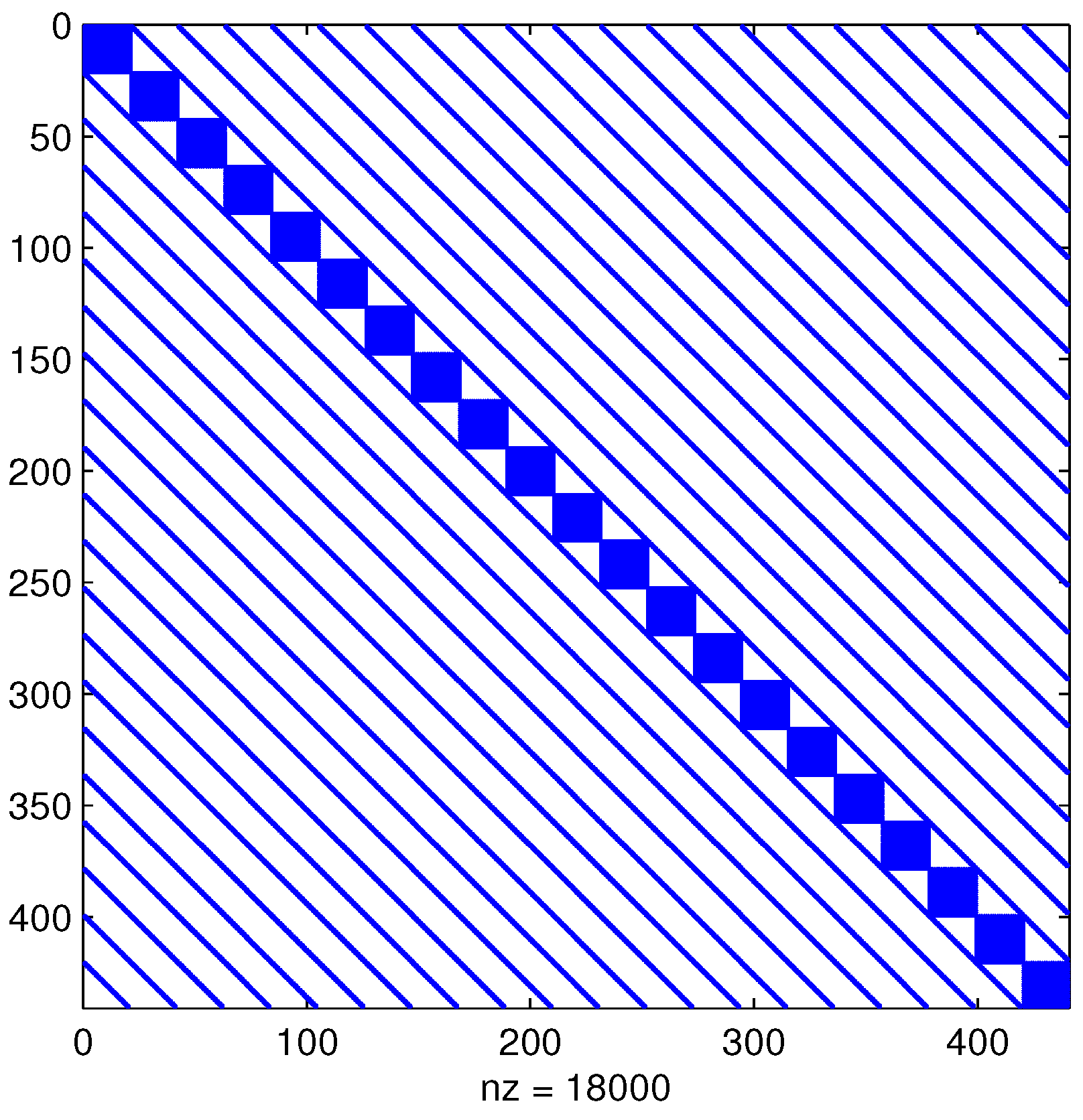
We first test a medium-size problem of order
.
Figure 1 illustrates the sparsity structure of the matrix
. This may show that for larger problems, it is expensive to compute the
factorization of
. For this experiment, as well as for the larger problems later, the final relative residual accuracy for both the LR-ADI method and the LR-Smith method was set to
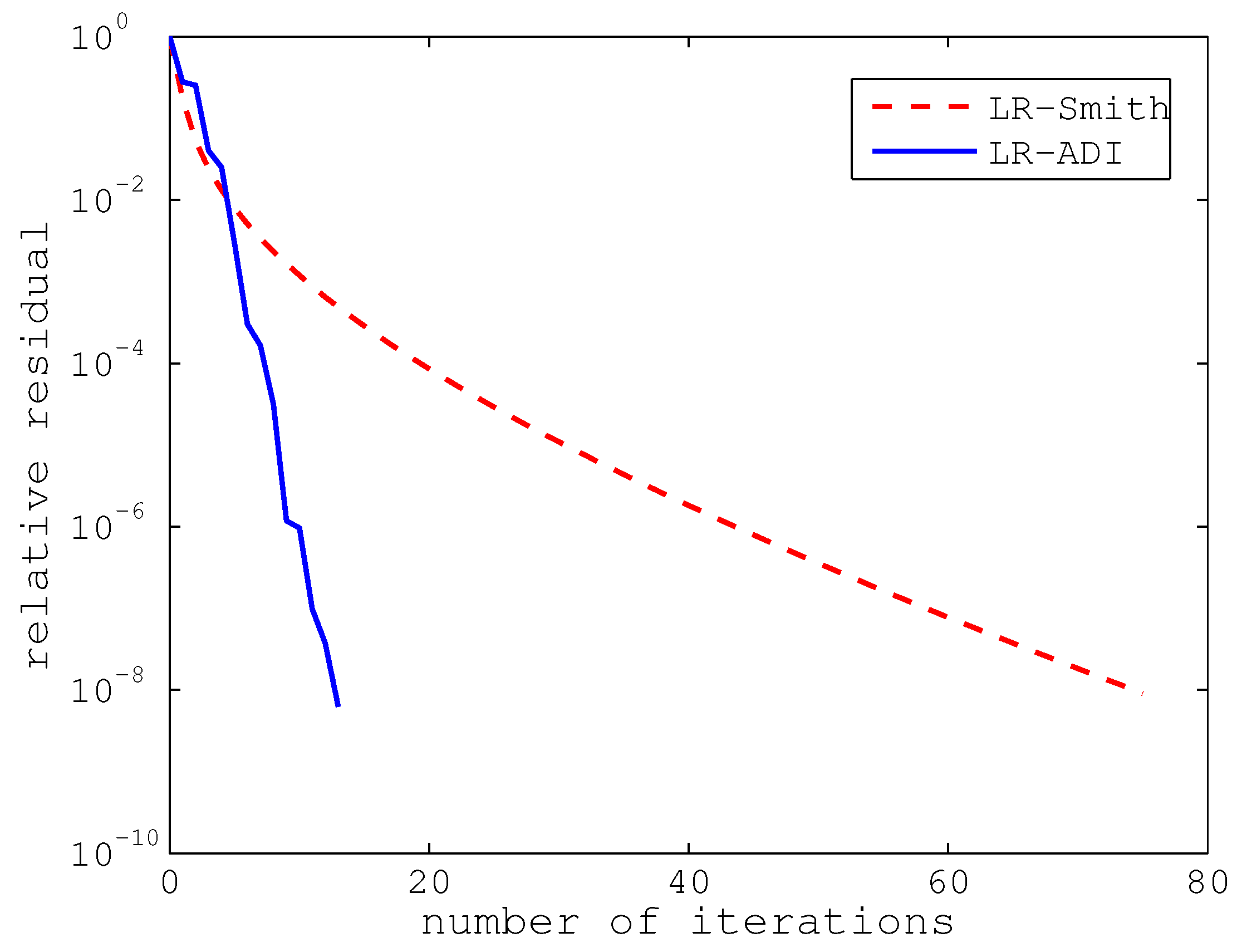
. The convergence curves of LR-ADI and LR-Smith are depicted in
Figure 2. The ADI method reaches a relative residual of 6.2472 ×
after 13 steps of iteration, while the Smith method has a relative residual of 9.1324 ×
after 75 steps. From
Figure 2, it is clear that LR-Smith is much slower than LR-ADI with respect to the number of iterations. From
Section 2, we know that the convergence factor of LR-Smith is the spectrum radius
. If the spectrum radius
, LR-Smith will converge very slowly. Note that the spectrum radius
is the absolute value of the largest finite eigenvalues (in modulus) of the pencil
. For this medium-size problem, the largest finite eigenvalue is 0.9554, which verifies the slow convergence of LR-Smith. However, from
Table 1, we can see that LR-Smith is only slightly more expensive, with respect to execution time, than LR-ADI. The reason is that linear systems with coefficient matrices
A and
must be solved in the latter method.
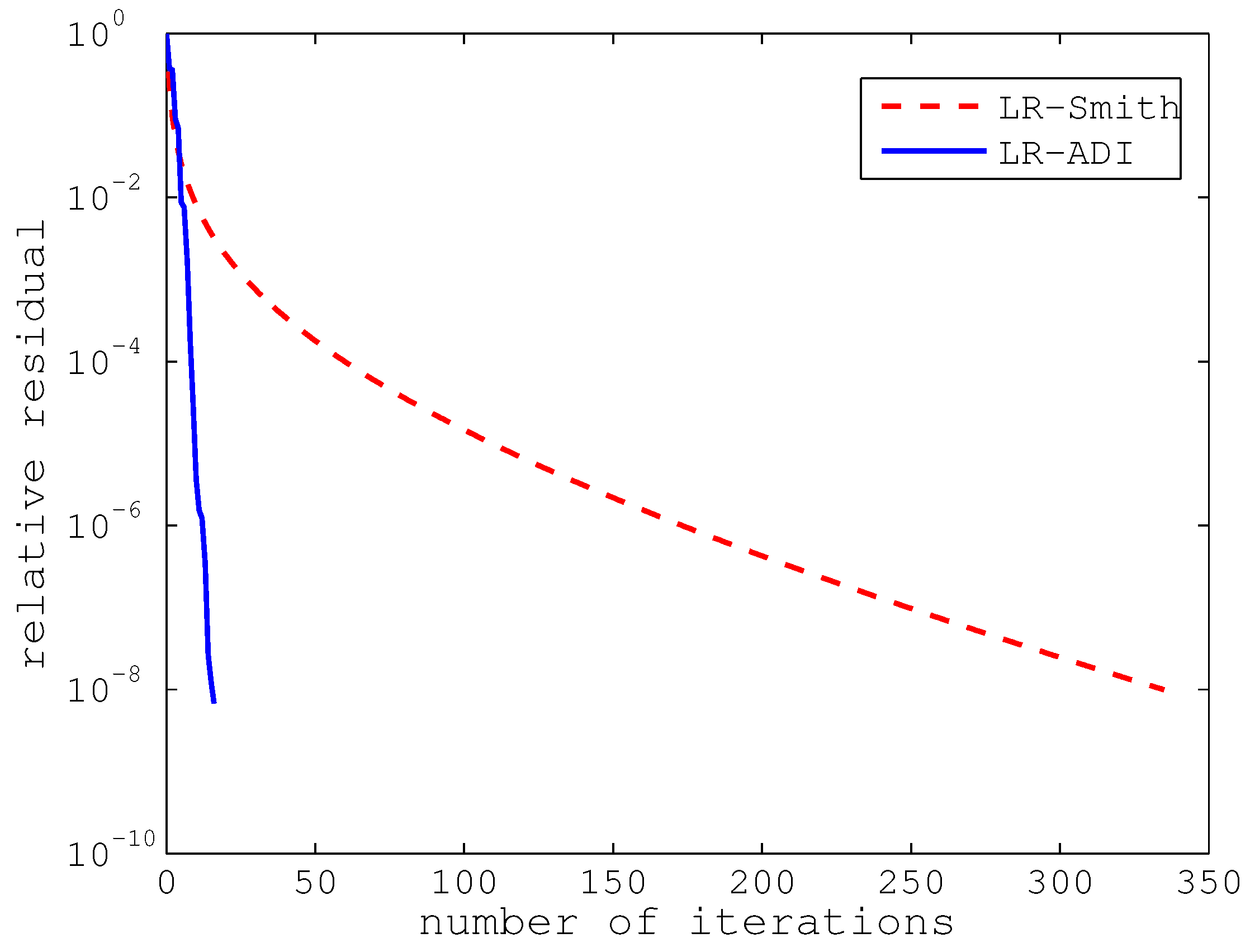
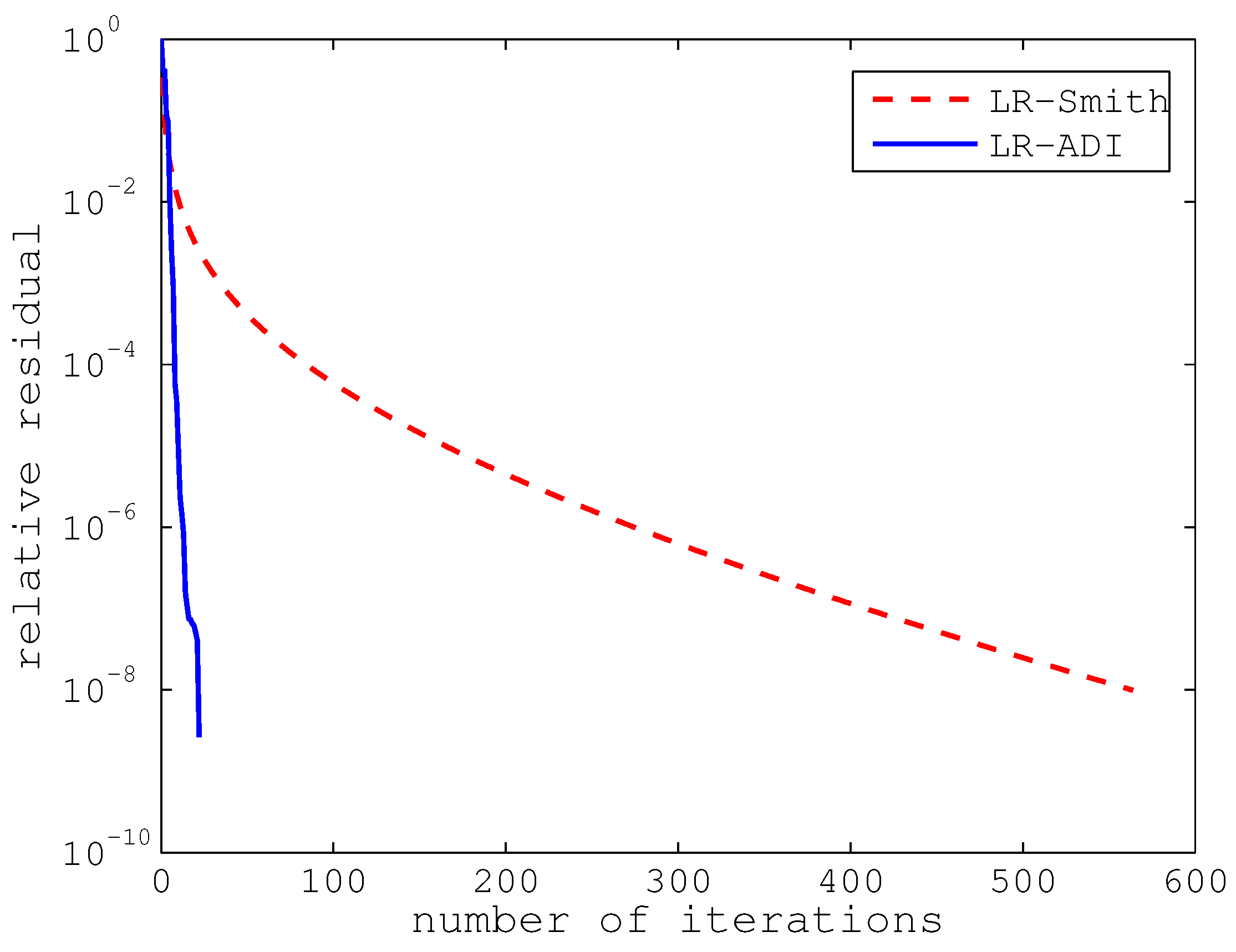
We also tested problems with larger dimensions, namely,
,
, and
n = 14,559. All the numerical results are reported in
Table 1. As expected, the execution time becomes increasingly larger for both LR-Smith and LR-ADI as the problem dimension expands. Moreover, it is clear that both the number of iterations and the cpu time of LR-ADI are better than those of LR-Smith. However, it is interesting that the number of iterations for LR-Smith increases much more dramatically than for LR-ADI. This is the reason that LR-ADI is more favorable with respect to the cpu time for problems with larger dimensions. For illustration, we also present the convergence curves of the two methods for dimensions
and
n = 14,559, respectively, in
Figure 3 and
Figure 4.
4.2. Example 2
In the second example, the DAE (
33) is used to describe a holonomically constrained damped mass–spring system with
g masses [
28,
37]. The system matrices have the following structures:
Similarly, we discretize the DAE by the same method as in the first example to obtain difference-algebraic equations, in which the matrices have the same block structures as in the first example.
By setting , 10,000, we obtain three DAEs of order , 12,001, 200,001. The timestep size is taken to be . All the elements of are set to 0, except the -th element, which is 1.
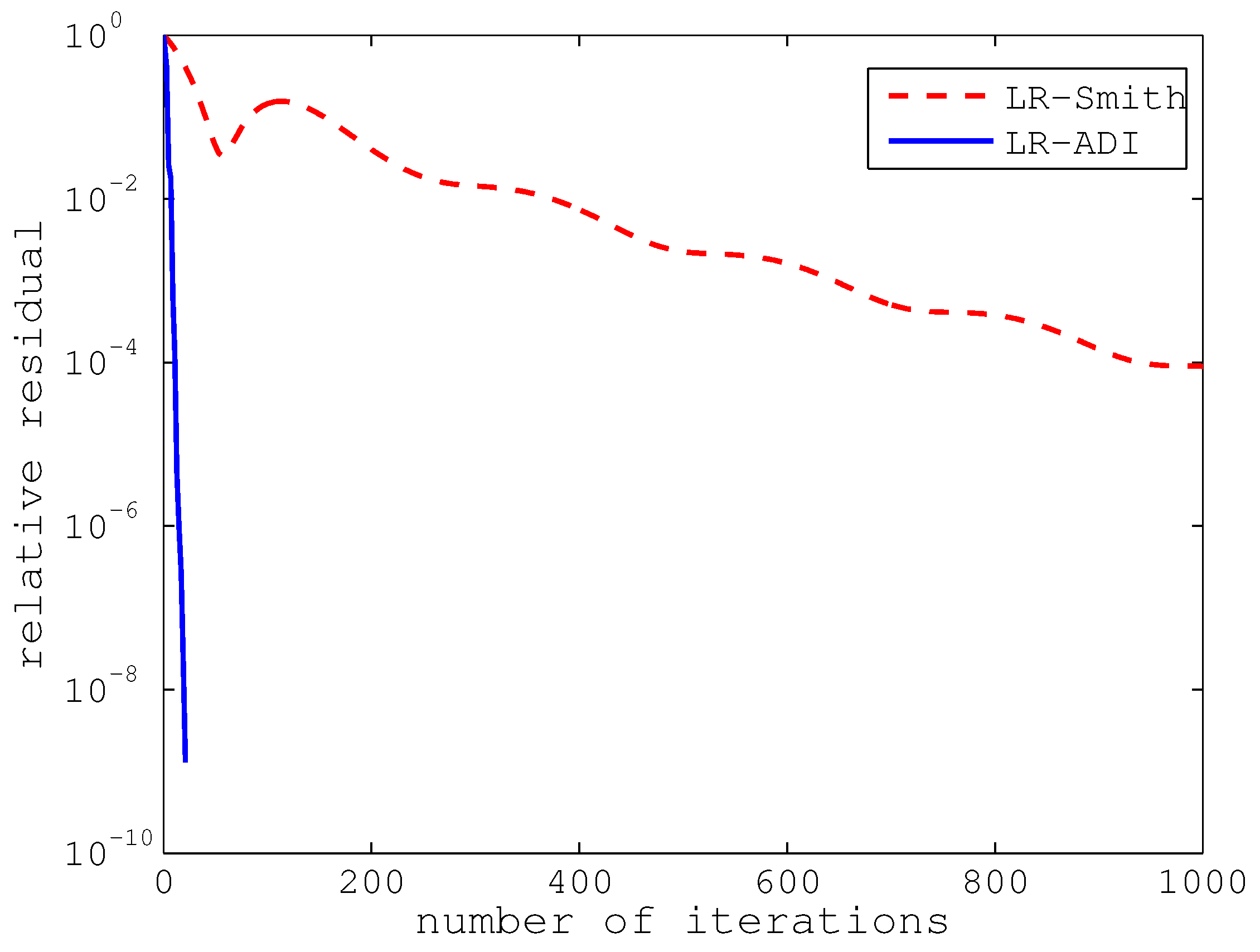
In
Figure 5, we first illustrate the convergence curves of LR-Smith and LR-ADI for the problem with the dimension
. Oddly enough, we can obviously see that the relative residual of LR-Smith does not monotonously decrease. This is due to the rounding error, which can make the relative residual strangely increase if the convergence factor is almost equal to 1. LR-Smith did not converge even if it had run 1000 steps, which cost 45.6 s. However, LR-ADI, with 21 steps of iteration, had a relative residual of 1.2886 ×
and a cpu time of 1.8 s.
Since LR-Smith does not converge for this example, we only report our numerical results of LR-ADI for all problems of different dimensions (
, 12,001, 20,001) in
Table 2. We observe that LR-ADI is very fast for this example and, in particular, that the number of iterations does not increase considerably with the expansion of the problem dimension. Moreover, we also notice that the execution time for this example is much less than that for the first example. The reason is that, in the second example,
is a number, and
are sparser than those in the first one, which makes it cheaper to compute the
factorization of
, and
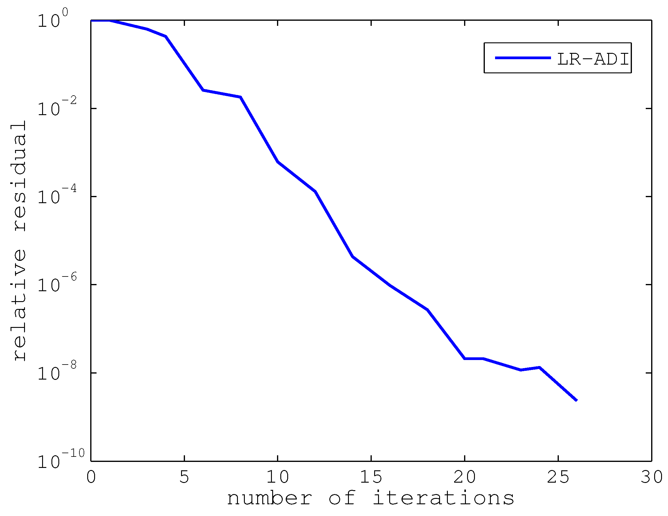
in this example. Finally, we show the convergence curve of LR-ADI for the problem with the dimension
n = 20,001 in
Figure 6.


