Stability Analysis and Hopf Bifurcation for the Brusselator Reaction–Diffusion System with Gene Expression Time Delay

Abstract

This paper investigates the effect of a gene expression time delay on the Brusselator model with reaction and diffusion terms in one dimension. We obtain ODE systems analytically by using the Galerkin method. We determine a condition that assists in showing the existence of theoretical results. Full maps of the Hopf bifurcation regions of the stability analysis are studied numerically and theoretically. The influences of two different sources of diffusion coefficients and gene expression time delay parameters on the bifurcation diagram are examined and plotted. In addition, the effect of delay and diffusion values on all other free parameters in this system is shown. They can significantly affect the stability regions for both control parameter concentrations through the reaction process. As a result, as the gene expression time delay increases, both control concentration values increase, while the Hopf points for both diffusion coefficient parameters decrease. These values can impact solutions in the bifurcation regions, causing the region of instability to grow. In addition, the Hopf bifurcation points for the diffusive and non-diffusive cases as well as delay and non-delay cases are studied for both control parameter concentrations. Finally, various examples and bifurcation diagrams, periodic oscillations, and 2D phase planes are provided. There is close agreement between the theoretical and numerical solutions in all cases.

1. Introduction and Preliminaries

In the last few decades, reaction–diffusion models have been applied to various nonlinear chemical applications, in particular, the Belousov–Zhabotinsky (BZ) reaction [1,2], the Brusselator model [3,4,5,6], the pellet model [7], the reversible Selkov model [8,9], and the Gray–Scott cubic autocatalytic model [10,11]. These have been used to examine many oscillatory phenomena in both theoretical studies and experiments, which typically employ a continuous-flow stirred-tank reactor (CSTR) [11,12,13,14,15].

A commonly studied chemical reaction model is the Brusselator system, which was introduced by [16] in 1968. Real-world applications of the Brusselator system occur in many physical and chemical settings, such as the formation of ozone from atomic oxygen, in enzymatic reactions, and in laser and plasma physics arising from multiple coupling between modes (see [17,18,19,20,21] and the references therein). The Brusselator model describes an autocatalytic chemical reaction with periodic limit cycle behavior. It has been applied in studies of the spatial distribution of morphogens and can provide insights into how multiple morphogens react to cells and patterns [22,23].

To demonstrate this chemical reaction system, we consider the Schnakenberg model [12,24], which is a two-species model for trimolecular reactions. This autocatalytic system has three important processing steps between two chemical outputs U and V (self-activating and reactant), and two input chemicals $A_{in}$ and $B_{in}$, as follows:

$$\begin{array}{c}\hfill A_{in}\rightleftharpoons U,2U+V\rightleftharpoons 3U,B_{in}⟼V.\end{array}$$

(1)

Hence, following [16,25], the well-known Brusselator model can be represented by four intermediate reaction processes as

$$\begin{array}{ccc}\hfill B_{in}& ⟼& U,\hfill \\ \hfill A_{in}+U& ⟺& V+D,\hfill \\ \hfill 2U+V& ⟼& 3U,\hfill \\ \hfill U& ⟼& E.\hfill \end{array}$$

(2)

where D and E are the outputs, while U and V are now intermediate chemicals. Suppose that $u(x,t)$ and $v(x,t)$ are the activator and inhibitor in the dimensionless concentrations of two reactants (interacting chemical species) at time t and that $\delta$ and $\gamma$ are two positive control concentrations through the reaction process $A_{in}$ and $B_{in}$, respectively. An autocatalytic process can produce both the Schnakenberg and the Brusselator models: the only difference between them is the number of chemical reactions that participate in the autocatalytic process (for more details, see [26]). Therefore, the non-dimensional form of chemical reaction process (2) can be represented as [3,27]

$$\begin{array}{ccc}\hfill & & \frac{\partial u}{dt}-{\mu }_1\Delta u=\delta -(\gamma +1)u+u^2\left(t\right)v\left(t\right),\hfill \\ & & \frac{\partial v}{dt}-{\mu }_2\Delta v=\gamma u-u^2\left(t\right)v\left(t\right),\hfill \end{array}$$

(3)

where ${\mu }_1$ and ${\mu }_2$ are the diffusion coefficients of two reactants. This form of diffusive Brusselator model has been considered and studied theoretically and numerically by many researchers; for example, see [3,5,17,20,28] and the references therein.

In this work, we are interested in adding a gene expression time delay ($\tau >0$) to the model (3) by applying a Dirichlet boundary condition. Including gene expression time delay in cellular pattern formation has a significant impact on the Brusselator system, so adding a delay can play a major role in generating spatially coordinated oscillations of gene expression [12,29]. A time delay can consequently move solutions in the model from stable to unstable and may create points of instability and bifurcation [29,30,31]. Hence, the model (3) can be rewritten as follows:

$$\begin{array}{ccc}\hfill & & \frac{\partial u}{dt}-{\mu }_1\Delta u=\delta -(\gamma +1)u+u^2(t-\tau )v(t-\tau ),\hfill \\ & & \frac{\partial v}{dt}-{\mu }_2\Delta v=\gamma u-u^2(t-\tau )v(t-\tau ),\hfill \\ & & u(x,t)=u_r\ge 0,v(x,t)=v_r\ge 0,\mathrm{when}(x,t)\in [0,1]\times [-\tau ,0],\hfill \\ & & u(x,t)=v(x,t)=0\mathrm{at}x=\pm 1.\hfill \end{array}$$

(4)

Here, all parameters $\delta$, $\gamma$, $\tau$, ${\mu }_1$, and ${\mu }_2$ are positive and have the same chemical meaning as in the above equations. This model in (4) is an open system and at the domain center, the zero-flux boundary condition was derived. Therefore, this model will exhibit symmetrical behavior at border points $x=\pm 1$ to the reservoir holding constant concentrations u and v at the reactor’s permeable boundary. In addition, $u_r>0$ and $v_r>0$ are realized here for examination as the system’s chemical concentrations u and v in $[-\tau ,0]$.

The diffusive Brusselator system with gene expression delay has been considered only in [29]. They derived the Turing instability and the Turing–Hopf bifurcation. The impact of the gene expression time delay in the model was explained: it can destabilize the positive constant steady state. Numerical examples were provided to support and examine the theoretical results. There have been few studies in the literature that concentrated on the diffusive Brusselator model with gene expression time delay. So far, no work has covered the full influence of gene expression time delay with diffusion parameters on stability, Hopf bifurcation regions, and bifurcation diagrams from both analytic and numerical perspectives. This is because most existing studies focus on a PDE model without delay [4,19,32]. This affords us motivation to conclude there is scope for additional research on the stability of this model. Therefore, this study contributes to the literature by examining the effect of gene expression time delay and diffusion on the model, especially on Hopf points, bifurcation diagrams, and regions of stability.

The work pursues several objectives: first, it aims to determine theoretical DDEs (delay differential equations) via the Galerkin method. This technique gives close approximations of delay DPDEs (delay-partial differential equations). The second objective is to explore, theoretically, a condition that assists in defining the existence of Hopf bifurcation points. From there, we derive the effects of two different diffusion rates as well as the gene expression time delay on the stability and Hopf bifurcation regions to discern how these diffusion coefficients interact with the time delay and the other free chemical control parameters. Numerical simulations and examples are sketched to display the bifurcation maps, limit-cycle oscillations, and 2D phase portraits to illustrate the theoretical findings.

The remainder of this paper is organized as follows. Section 2 shows the Galerkin method and the dynamical theoretical framework. In addition, the theoretical condition to find the Hopf bifurcation points is derived. In Section 3, we draw Hopf bifurcation maps for stability analysis, investigating both the theoretical and numerical outputs. We also discuss how the two different rates of diffusion with delay sources interact with the other free parameters in this model. In Section 4, we construct the bifurcation diagram and 2D limit cycle for the DDE and DPDE systems, using long-term numerical simulations to confirm and gain deeper insight into the theoretical results.

2. The Galerkin Method

Various analytical methods can be used to solve nonlinear PDE models; however, some of them have proven unable to find solutions reliably. Here, we examine and utilize a method that has been applied successfully to PDEs with delays, named the Galerkin analytical method [33]. This method can be used to create a system of ODEs or DDEs corresponding to a given nonlinear delay PDE system.

The Galerkin method has been employed in many complex applications with reaction-diffusion models, such as the pellet problem [7], the Lotka–Volterra predator–prey model [9,34], the viral infection system [35], the Schnakenberg system [12], the Gray–Scott cubic autocatalytic system [11], the BZ equation [1] and Nicholson’s blowflies equation [36] etc. Overall, the approach has yielded reliable results and good agreement between analytic and numerical outputs.

Our DDE system can be derived from the delay PDE model (4) by applying the following trial equations:

$$\begin{array}{ccc}\hfill & & u_{(x,t)}=u_{1\left(t\right)}cos{z}_1+u_{2\left(t\right)}cos{z}_2,\hfill \\ & & v_{(x,t)}=v_{1\left(t\right)}cos{z}_1+v_{2\left(t\right)}cos{z}_2,\hfill \\ & & \mathrm{where}{z}_1=\frac{1}{2}\pi x\mathrm{and}{z}_2=\frac{3}{2}\pi x.\hfill \end{array}$$

(5)

The expansions of the trial equations are selected so that $u_{(x,t)}=\sum u_{i\left(t\right)}$ and $v_{(x,t)}=\sum v_{i\left(t\right)}$ are the concentrations at the center of the chemical reaction–diffusion model. The boundary conditions at $x=\pm 1$ are satisfied [11,36]. The trial expansions in (5) meet the boundary conditions in the delay PDE system in (4). Note, that the delay PDE in (4) is not satisfied exactly, but the free parameters in this consideration are established by computing averaged versions of the governing equations in (5). Then, each equation in (4) is weighted by the two trial functions $cos{z}_1$ and $cos{z}_2$. After that, a system of four ODEs with delay is obtained. This system of equations is called an analytical (theoretical) equation of the two-term scheme. This system is set out in the Appendix A.

The series in (5) were cut to the two-term trial equations, as this provided sufficient accuracy without overly complicating them, as measured by agreement with the system of the delay PDE numerical simulation. Furthermore, the analytical outcome of the delay ODE for the one-term solution provides a reasonably accurate result, as we will see in Section 4. This can be found by setting $v_2=u_2=0$ in the system (A1).

3. The Dynamical Theoretical Formulation

In this section, we discuss a theoretical framework that can be used to display the Hopf bifurcation points theoretically via a delay ODE system (A1). These points consist of curves that can divide the stability regions into stable and unstable zones. As the Hopf bifurcation point is approached, the periodic oscillations of limit cycles reach close to an equilibrium point of the steady state, and then the system goes from stable to unstable. This transition is associated with a conjugate pair of eigenvalues passing over the imaginary axis [37,38,39,40,41]. Hence, the Hopf bifurcation points can be found from the Taylor series at the steady state as

$$\begin{array}{cc}\hfill & u_j=u_{js}+ϵ{\nu }_1{e}^{-rt},v_j=v_{js}+ϵ{\nu }_2{e}^{-rt}\mathrm{where}j=1,2\mathrm{and}ϵ\ll 1.\end{array}$$

(6)

By substituting these variables into the delay ODE equations (A1), the associated Jacobian matrix $J_j$ can be obtained as

$$J_j=\left[\begin{array}{cccc}{\displaystyle \frac{\partial {\chi }_1}{\partial u_1}}-r& {\displaystyle \frac{\partial {\chi }_1}{\partial v_1}}& {\displaystyle \frac{\partial {\chi }_1}{\partial u_2}}& {\displaystyle \frac{\partial {\chi }_1}{\partial v_2}}\\ {\displaystyle \frac{\partial {\chi }_2}{\partial u_1}}& {\displaystyle \frac{\partial {\chi }_2}{\partial v_1}}-r& {\displaystyle \frac{\partial {\chi }_2}{\partial u_2}}& {\displaystyle \frac{\partial {\chi }_2}{\partial v_2}}\\ {\displaystyle \frac{\partial {\chi }_3}{\partial u_1}}& {\displaystyle \frac{\partial {\chi }_3}{\partial v_1}}& {\displaystyle \frac{\partial {\chi }_3}{\partial u_2}}-r& {\displaystyle \frac{\partial {\chi }_3}{\partial v_2}}\\ {\displaystyle \frac{\partial {\chi }_4}{\partial u_1}}& {\displaystyle \frac{\partial {\chi }_4}{\partial v_1}}& {\displaystyle \frac{\partial {\chi }_4}{\partial u_2}}& {\displaystyle \frac{\partial {\chi }_4}{\partial v_2}}-r\end{array}\right]$$

(7)

The Jacobian’s eigenvalues r appear where small perturbations develop in the model. The characteristic polynomial equation is derived by setting $r=j\omega$, and dividing the characteristic polynomial equation into two parts: the real ℜ and imaginary ℑ parts. The bifurcation condition can then be obtained by estimating the following equation:

$${\chi }_j=\Re =\Im =0,\mathrm{where}j=1,2,3,4.$$

(8)

The fourth-order Runge–Kutta Method (fourth) [42,43] is commonly used to solve ODEs or DDEs numerically; however, the Crank–Nicolson technique [36] is used to find solutions of the governing PDEs or DPDEs (4). The spatial and temporal discretizations in this work are based on $\Delta x=0.005$ and $\Delta t=0.0001$. The ratio of error is used to illustrate the difference between the theoretical outcomes and the numerical results and is defined as the ratio between the difference and the actual results, expressed as a percentage. In this work, we consider $u_r=v_r=0.05$ as positive chemical initial concentrations in all the numerical investigations. However, changing the initial concentration values $u_r$ and $v_r$ does not affect the region of stability. The effect of changing these values is limited: it may lead to different initial relaxation oscillations, but the stability region (the Hopf curve) should be the same. All numerical results for simulations of both DDE and DPDE systems are found using theMaple software package(12) [44].

4. Hopf Bifurcation

This section considers the effect of gene expression time delay and diffusion on the Hopf bifurcation points and stability regions. The results of both analytical solutions of the DDEs (A1) and numerical solutions of the DPDEs (2) are presented. In addition, we construct full plots of the Hopf point curves and examine the stable and unstable regions, illustrating them with numerical examples. Moreover, we characterize the influence of the two different diffusion and gene expression time delay values, and the other chemical control parameters $\gamma$ and $\delta$, on the stability regions during the reaction process. The Hopf bifurcation curve for the diffusive and non-diffusive systems as well as the delay and non-delay cases will be considered for positive control rates $\gamma$ and $\delta$.

Figure 1 shows diagrams of two different stability zones of the Hopf points, for the gene expression time delay $\tau$ against concentrations of input reagents $\delta$ (left panel) and $\gamma$ (right panel). In each plot, there is an upper unstable region and a lower stable region. Both show that as the impact of gene expression is subjected to greater time delays $\tau$, the Hopf bifurcation points for both chemical concentration rates $\delta$ and $\gamma$ increase. It can also be seen that the differences between Hopf points at large values of gene expression time delay are extremely small. The theoretical prediction of the DDE system agrees with the numerical DPDE outputs, with discrepancies below $1\%$ at the end of the x-axis ($\tau$) domain. Hence, it is evident that the gene expression delay time $\tau$ exerts a strong impact on the bifurcations and stability regions for both chemical concentration rates considered ($\gamma$, $\delta$) during the reaction process, and that modifying the value of $\tau$ can shift the model into or out of the stability region [1,12].

Figure 2a shows the Hopf bifurcation regions for the gene expression time delay $\tau$ against the diffusion coefficient $\mu$, with the blue crosses representing numerical DPDE solutions, while the dotted lines represent DDE analytic solutions for one-term (red dashed lines) and two-term (black solid lines) approximations. Figure 2b shows the effect of three values of the chemical control $\gamma \in \{3,4,5\}$ on the stability regions of the Hopf points. As in Figure 1, an upper stable region and a lower unstable region are found. It can be seen that the diffusion parameter $\mu$ reduces slowly as the gene expression time delay $\tau$ increases. For any fixed value of $\tau$, $\mu$ increases as the chemical control $\gamma$ decreases. In other words, increasing the rate of chemical control $\gamma$ reduces the region of instability and increases stability regions.

Figure 3a shows the Hopf bifurcation regions in the $\delta$– $\gamma$ plane, with the DPDE numerical solutions shown as blue crosses and the DDE analytical solutions for one-term and two-term approximations shown as red dashed and black solid lines, respectively. Figure 3b compares the Hopf bifurcation curves for four example diffusion rates, $\mu \in \{0.15,0.20,0.25,0.30\}$, based on the two-term analytical results for the DDE system at $\tau =1$. Both maps present two stability regions (one stable and one unstable). It appears that, as the control rate $\delta$ grows, the chemical control $\gamma$ increases linearly. Furthermore, Figure 3b shows that, at any given $\delta$, the values of the control $\gamma$ rise with the increasing diffusion parameter $\mu$. In addition, Figure 4 shows the regions of the Hopf bifurcation maps for the $\delta$–$\mu$ (left panel) and $\gamma$–$\mu$ (right panel) planes. Shown in both figures are theoretical results for the DDE equations. As before, two stability zones can be seen. Following the bifurcation curve, as the diffusion values increase, the chemical control $\delta$ increases linearly, while it decreases steadily as $\gamma$ increases.

Figure 5 shows the three cases of Hopf bifurcation zones in the ${\mu }_1$–${\mu }_2$ plane for four values of $\tau$ (upper panel), $\delta$ (middle panel), and $\gamma$ (lower panel). These plots are based on the theoretical two-term DDE results. The parameters applied here are as follows: $\delta =\gamma =2$ in Figure 5a, $\tau =10$ and $\gamma =2$ in Figure 5b, and $\tau =10$ and $\delta =5$ in Figure 5c. An unstable area can also be seen above each curve and a stable region below. The results in all cases reveal that with an increase in the diffusion rate ${\mu }_1$, the diffusion rate ${\mu }_2$ decreases and the Hopf bifurcation points are moved from left to right. In addition, in Figure 5a,b, at any fixed value of ${\mu }_1$, the Hopf bifurcation points for ${\mu }_2$ increase as the time delay $\tau$ or chemical control rate $\delta$ are increased. However, it can be seen in Figure 5c that at any fixed diffusion rate ${\mu }_1$, the value of ${\mu }_2$ decreases as the chemical control value $\gamma$ grows.

Figure 6a compares the $\delta$–$\gamma$ Hopf bifurcation curves for two cases: with delay ($\tau =1$) and without delay ($\tau =0$). A positive diffusion rate of $0.05$ is assumed. In this figure, adding time delay shifts the bifurcation curve downward for the value of $\gamma$ with a fixed $\delta$. The chemical control rate $\gamma$ grows as the value of $\delta$ increases for both cases. Figure 6b,c show $\omega$–$\delta$ plots with a delay case ($\tau =1$–black solid curve) and a non-delay case ($\tau =0$–red solid curve). The frequency $\omega$ of the periodic oscillation increases, and the values of $\delta$ rise with the non-delay case in Figure 6b. However, in Figure 6c, $\delta$ is reduced in the delay case.

Figure 7a shows the Hopf bifurcation regions in the $\delta$–$\gamma$ plane for two values of the diffusion rates: a non-diffusion case ($\mu =0$) and a positive-diffusion case at ($\mu =0.1$) with gene expression time delay equal to $\tau =1$. This figure shows that at a fixed chemical control value $\delta$, the Hopf bifurcation points are increased as one shifts from the non-diffusion case to the positive-diffusion case. Figure 7b presents the chemical control value concentration of $\delta$ against the frequency $\omega$ of the limit cycle for the same two cases as Figure 7a. The frequency $\omega$ in Figure 7b decreases as $\delta$ increases. The frequency falls more quickly in the non-diffusion case than in the diffusion case.

In general, the different diffusion and delay rates have a significant influence and can move the Hopf points and change the stability of this system.

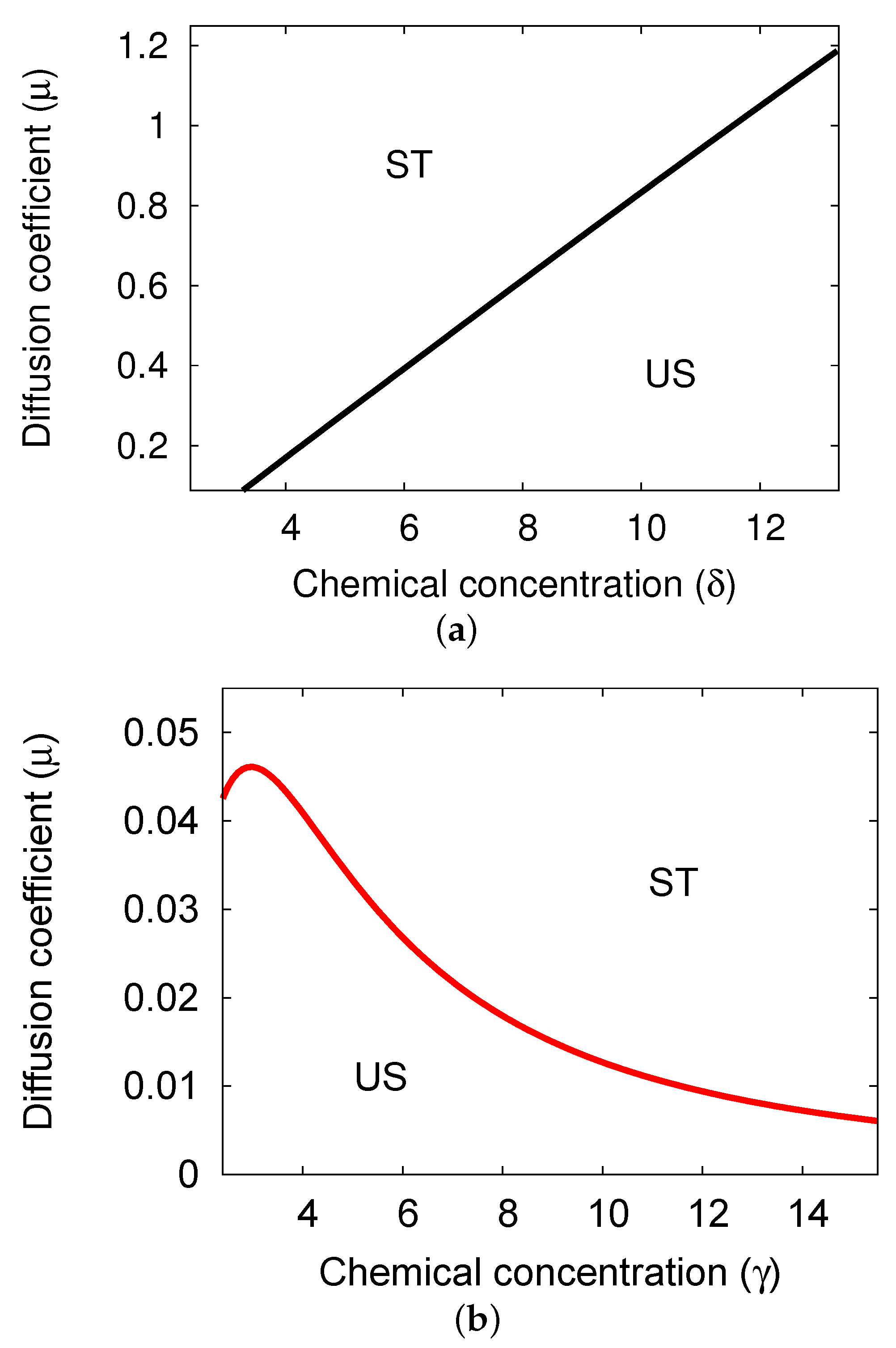
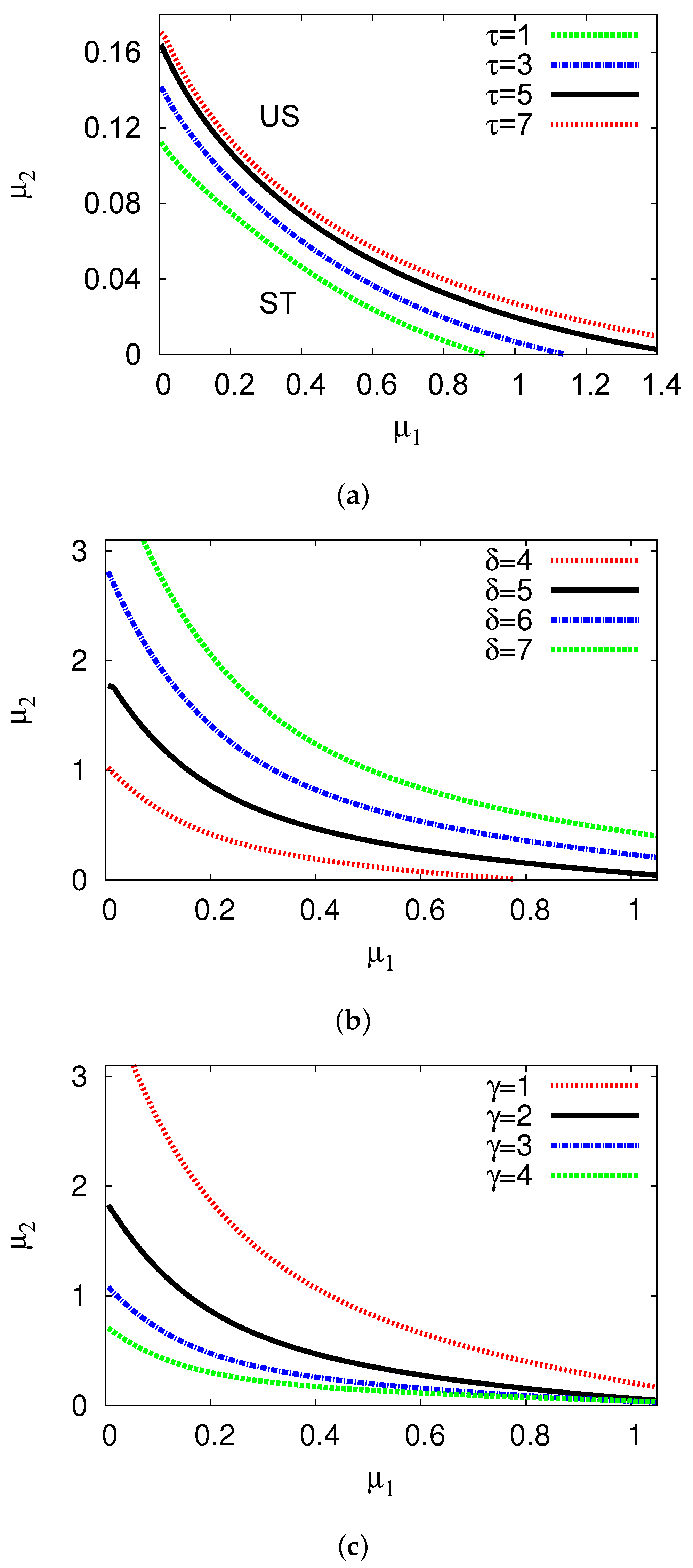
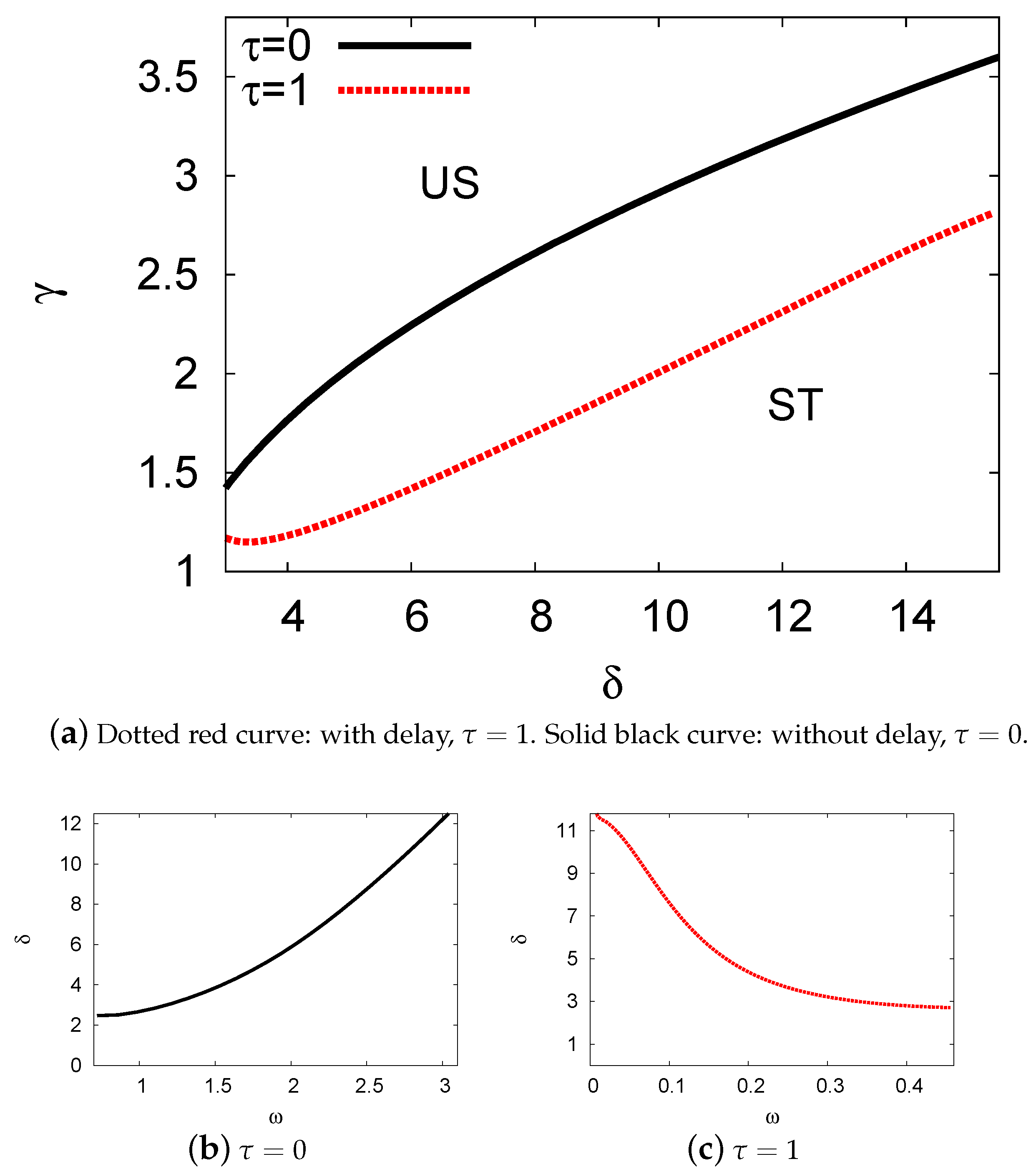
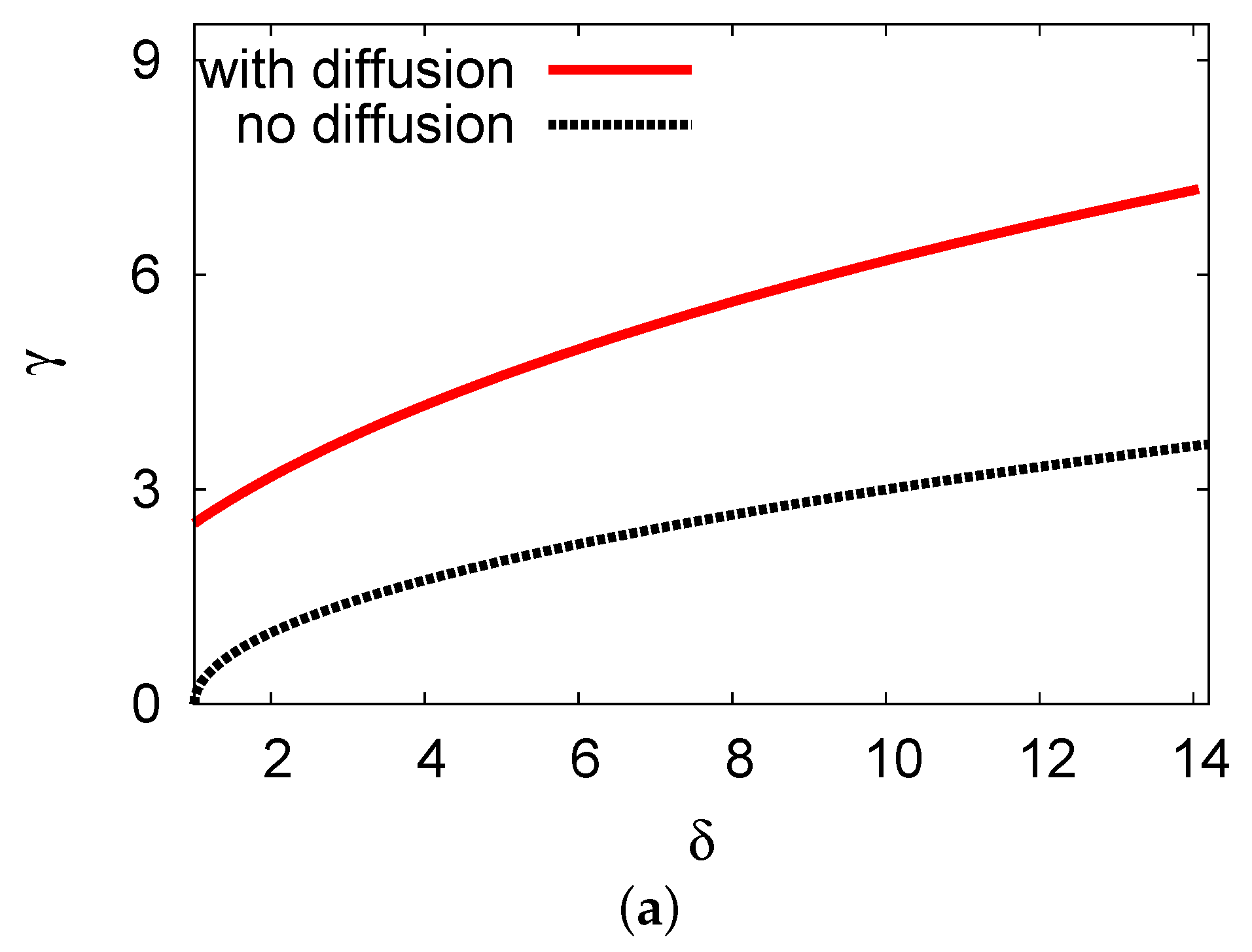
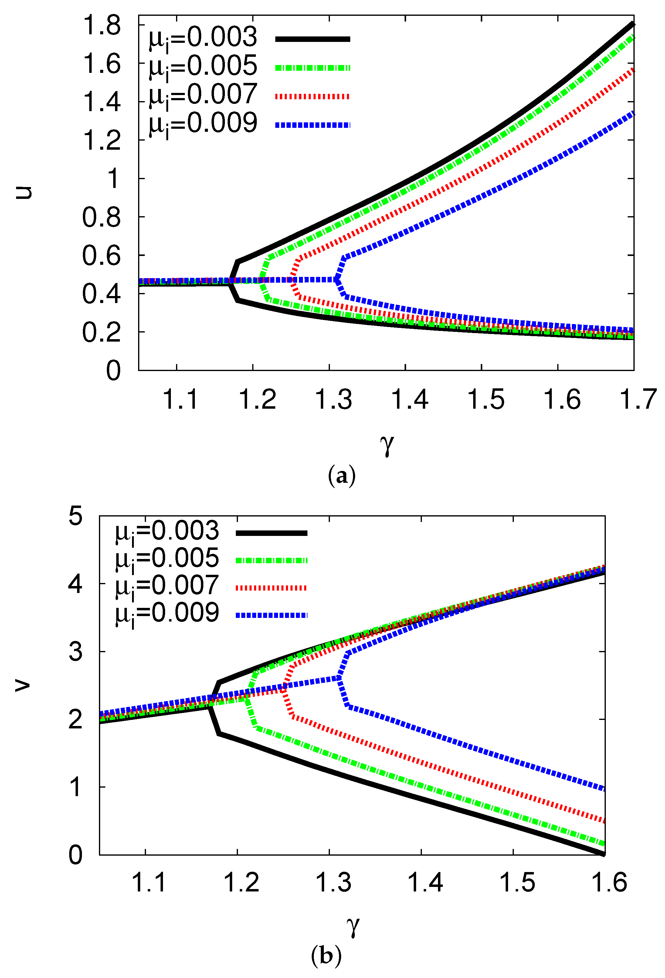
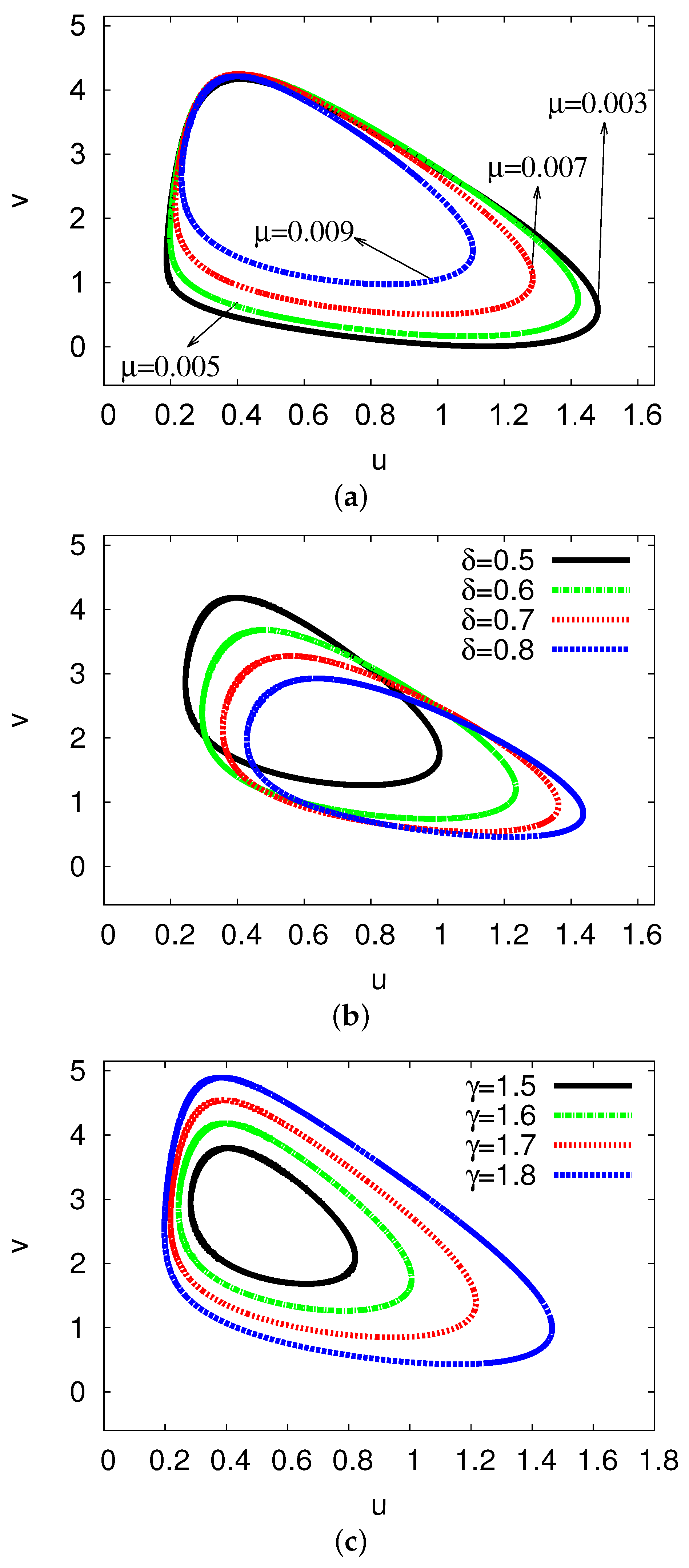
5. Bifurcation Diagrams

This section presents bifurcation diagrams that demonstrate the complex periodic behavior of this model for both approaches: DDEs as in (A1) and DPDEs as in (4). A bifurcation diagram shows the values visited or approached asymptotically, and can be interpreted as displaying behaviors such as fixed points, periodic orbits, and chaotic attracts. In addition, different examples of periodic oscillation for both concentrations of the intermediate products u (the activator) and v (the inhibitor) are plotted to characterize the impacts of the free parameters (${\mu }_i,\tau ,\gamma$). Throughout this section, numerical simulations will be exhibited to emphasize the analytical stability of the Hopf bifurcation region.

5.1. Bifurcation Diagrams at $\tau =0$

The steady-state numerical bifurcation diagrams for the two chemical concentrations u and v for the non-delay case at $\tau =0$, have been explored in the literature by many researchers. In [4,5], steady-state solutions were found by using outputs of both the analytical ODEs and the numerical PDE Brusselator system at $\tau =0$, which can be obtained by substituting the equations

$$\begin{array}{c}\hfill \begin{array}{cc}\hfill v_{js\left(t\right)}& =v_{j(t-\tau )},u_{js\left(t\right)}=u_{j(t-\tau )}\mathrm{where}j=1,2.\hfill \end{array}\end{array}$$

(9)

into both systems of DDEs (A1) and DPDEs (4). The results presented in these papers show that there are unique patterns of steady-state outcomes for the concentrations of the activator u and inhibitor v. It was also found that as the control parameter $\gamma$ increases, the dimensionless concentration of the activator u reduces, while the control $\gamma$ increases with the concentration of the inhibitor v. For more information about simulations of steady-state behaviors, see [4,5] and the references therein.

5.2. Bifurcation Diagrams at $\tau >0$

Figure 8a,b show bifurcation diagrams of the $\gamma$–u (left panel) and $\gamma$–v planes (right panel). Solutions are derived for both the theoretical DDEs (black line) and a numerical scheme for the DPDEs (red dots) is derived. These plots demonstrate the importance of the gene expression time delay $\tau$ in the system, which can move the solutions between stable and unstable long-term behavior. The long-term results are stable for the chemical concentrations u and v for control values $0<\gamma <{\gamma }_{hopf}$. After this point, the periodic results of a supercritical Hopf bifurcation are seen. Therefore, the Hopf bifurcation point for the numerical simulation of the DPDE system is $\gamma \simeq 1.32$, while in the theoretical two-term result, the bifurcation point is at $\gamma \simeq 1.35$. Beyond the Hopf point of the chemical control ${\gamma }_{hopf}$, $\gamma$ grows, the oscillation of the limit cycle increases, and the other branch of the minimum amplitude drops down. The theoretical solutions of the two-term result match with predictions of the numerical DPDE system at both concentrations.

Figure 9a,b show the time evolution of u and v, respectively, plotted at the center of the domain when $\gamma$ = 1.2 (from the stable region in Figure 8). Figure 9c shows a 2D phase portrait map for concentration u against v. This figure shows that $\gamma =1.2<{\gamma }_{hopf}$ and that the result at this point converges to a stable steady state at $(u,v)\simeq (0.48,2.41)$, after a transient and a few periodic oscillations. There is an agreement between the analytical DDE system and numerical delay PDE solutions, within $4\%$ at time $t=250$. Figure 10 shows the behavior of limit cycles for the two concentrations over the same long time duration. The parameters used in this example are the same as in Figure 9, with chemical control $\gamma =1.6$, and this point is selected after the Hopf point in Figure 8. At this selected fixed point, the periodic outputs continue through the entire time duration. The oscillation amplitudes are $(u,v)=(1.02,4.19)$ and $(u,v)=(1.17,4.22)$ for the theoretical DDE and numerical DPDE solutions, respectively. Furthermore, the cycle periods are $27.89$ and $26.95$ for the DDE and DPDE solutions, respectively, the numerical scheme agrees with the theoretical outcomes for the cycle period with a discrepancy of less than $3.5\%$.

Figure 11a,b depict bifurcation diagrams of the concentrations u and v with respect to the chemical control parameter $\gamma$, using the two-term analytical solutions with four values of diffusion the coefficients: $\mu =0.003$ (black solid line), $0.005$ (green dashed line), $0.007$ (red dotted line), and $0.009$ (blue dashed line). The positive values that were used here are $\delta$ = 0.5 and $\tau =1$. The Hopf bifurcation points for both chemical concentrations u and v are at ${\gamma }_{hopf}\simeq 1.18,1.22,1.26$, and $1.31$ for $\mu =0.003,0.005,0.007,$ and $0.009$, respectively. It is apparent that decreasing the diffusion coefficient rate stabilizes the model while increasing $\mu$ causes both chemical concentrations u and v to go forward. The effect of the diffusion coefficient $\mu$ on the control parameter $\delta$ shows the same behavior as with the control $\gamma$.

Figure 12 shows 2D phase maps in the u–v plane for four different examples of the rates $\mu$ (left panel), $\delta$ (right panel), and $\gamma$ (lower panel). The two-term analytical solutions are explored in all cases, with $\gamma$ = 1.6, $\delta$ = 0.5, and $\tau =1$ in Figure 12a; $\gamma$ = 1.6, $\mu$ = 0.01, and $\tau =1$ in Figure 12b and $\mu =0.01$, $\delta =0.5$, and $\tau =1$ in Figure 12c. In Figure 12a, the periods of the limit cycles for $\mu =0.003,0.005,0.007$, and $0.009$ are $27.53,27.01,26.80$, and $26.60$, respectively. In contrast, we can see in Figure 12a that increasing the diffusion rate $\mu$ reduces the oscillation time slightly. However, Figure 12b shows that as $\delta$ increases, the oscillation period lengthens slowly. Furthermore, it is clear in Figure 12c that the oscillation period grows rapidly as the rate $\gamma$ is increased. For the orbits presented in Figure 12c, the long periods for $\gamma =1.5,1.6,1.7$, and $1.8$ are equal to $26.75,27.89,29.08$, and $30.25$, respectively. These results confirm the solutions in the outcome of Figure 11. In summary, both chemical controls with delay as well as diffusion coefficient values are significant in this system and can affect the stability and Hopf points.

5.3. Examples and Numerical Simulations at Long Delay Time

In this subsection, numerical simulations are obtained at long gene expression time delay $\tau$, validating the analytical results with the numerical outcomes. One significant reason for studying large values of the gene expression time delay is to check if the system has a period-doubling and chaotic outcome. Here, we discuss the exact value of the Hopf bifurcation point for the chemical concentration rate $\delta$ for six different long-time delay values, as presented in

Table 1. Comparison between the theoretical results of DDEs (A1) and a numerical scheme of DPDEs (4) for six Hopf points for chemical rates $\delta$.

Case	1-DDEs	2-DDEs	DPDEs
$\tau =50$	1.998	1.995	1.996
$\tau =100$	1.999	1.996	1.997
$\tau =150$	2.000	1.999	2.000
$\tau =200$	2.002	2.004	2.005
$\tau =250$	2.004	2.009	2.011
$\tau =300$	2.005	2.011	2.013

. The other positive parameters are ${\mu }_i=0.05$ and $\gamma =10$. The results in the table show that, as $\tau$ increases, the difference between the Hopf bifurcation points increases slowly, with less than a ≃0.1% error between them. All these instances occur beyond the Hopf bifurcation point. Moreover, many chemical systems such as Nicholson’s blowflies [36], the Schnakenberg model [12,45] and the delayed immune model [46] displays period-doubling and chaotic results. In our case, a chaotic solution does not occur in either the DPDE equations or the DDE system.

6. Conclusions and Outlook

This paper discussed both analytical and numerical approaches to solving the Brusselator reaction–diffusion system with gene expression time delay. The Galerkin technique was used to obtain a system of DDEs. The stability and Hopf bifurcation regions were obtained both theoretically and numerically. We sketched full bifurcation diagrams for the two different diffusion rates and the delay time, displaying their relationships with the other free parameters in the context of the reaction chemical process. The Hopf bifurcation diagrams showed two different stability regions. The gene expression delay time, as well as diffusion coefficient values, strongly influence the stability and bifurcation results in this model. It was found that the Hopf bifurcation points for both chemical concentration rates increase as the gene expression time delay grows. In addition, with raised gene expression time delay values, the Hopf points for both diffusion coefficients were reduced. Moreover, the Hopf bifurcation diagrams for the diffusive and non-diffusive cases and delay and non-delay cases were discussed for two positive control concentrations $\delta$ and $\gamma$. The findings here revealed that the rates of the diffusion and delay cases have higher Hopf points than the non-diffusion and non-delay cases, respectively. Bifurcation diagrams and 2D maps for the activator and inhibitor were also drawn to examine their impacts on the reaction process. Comparing the DDE two-term theoretical solutions to the numerical simulation DPDE scheme demonstrated the benefits of this technique, which yielded realistic and logical results in all cases studied. In future work, the approach could be applied to study and explain the behavior of other PDE systems with delays.

References

1. Alfifi, H.Y.; Marchant, T.R.; Nelson, M.I. Non-smooth feedback control for Belousov-Zhabotinskii reaction-diffusion equations: Semi-analytical solutions. J. Math Chem. 2016, 57, 157–178. [Google Scholar] [CrossRef]
2. Ren, J.; Gao, J.; Yang, W. Computational simulation of Belousov-Zhabotinskii oscillating chemical reaction. Comput. Visual Sci. 2009, 12, 227–234. [Google Scholar] [CrossRef]
3. Adomian, G. The diffusion-Brusselator equation. Comput. Math. Appl. 1995, 29, 1–3. [Google Scholar] [CrossRef]
4. Alfifi, H.Y. Semi-analytical solutions for the Brusselator reaction-diffusion model. ANZIM J. 2017, 59, 167–182. [Google Scholar] [CrossRef]
5. Alfifi, H.Y. Feedback Control for a Diffusive and Delayed Brusselator Model: Semi-Analytical Solutions. Symmetry 2021, 13, 725. [Google Scholar] [CrossRef]
6. Guo, G.; Wu, J.; Ren, X. Hopf bifurcation in general Brusselator system with diffusion. Appl. Math. Mech. Engl. Ed. 2011, 32, 1177–1186. [Google Scholar] [CrossRef]
7. Marchant, T.R.; Nelson, M.I. Semi-analytical solution for one-and two-dimensional pellet problems. Proc. R. Soc. Lond. 2004, A460, 2381–2394. [Google Scholar] [CrossRef]
8. Al Noufaey, K. A semi-analytical approach for the reversible Schnakenberg reaction diffusion system. J. Results Phys. 2020, 16, 102858. [Google Scholar] [CrossRef]
9. Al Noufaey, K.S.; Marchant, T.R. Semi-analytical solutions for the reversible Selkov model with feedback delay. Appl. Math. Comput. 2014, 232, 49–59. [Google Scholar] [CrossRef]
10. Alharthi, M.R.; Marchant, T.R.; Nelson, M.I. Mixed quadratic-cubic autocatalytic reaction-diffusion equations: Semi-analytical solutions. Appl. Math. Model. 2014, 38, 5160–5173. [Google Scholar] [CrossRef]
11. Marchant, T.R. Cubic autocatalytic reaction diffusion equations: Semi-analytical solutions. Proc. R. Soc. Lond. 2002, A458, 873–888. [Google Scholar] [CrossRef]
12. Alfifi, H. Stability analysis for Schnakenberg reaction-diffusion model with gene expression time delay. Chaos Solitons Fractals 2022, 155, 111730. [Google Scholar] [CrossRef]
13. Gray, P.; Griffiths, J.F.; Scott, K. Branched-chain reactions in open systems: Theory of the oscillatory ignition limit for the hydrogen+ oxygen reaction in a continuous-flow stirred-tank reactor. Proc. R. Soc. Lond. 1984, A394, 243–258. [Google Scholar]
14. Gu, Y.; Ullah, S.; Khan, M.A.; Alshahrani, M.Y.; Abohassan, M.; Riaz, M.B. Mathematical modeling and stability analysis of the COVID-19 with quarantine and isolation. Results Phys. 2022, 34, 105284. [Google Scholar] [CrossRef] [PubMed]
15. Liu, J.; Zhang, Q.; Tian, C. Effect of Time Delay on Spatial Patterns in a Airal Infection Model with Diffusion. Math. Model. Anal. 2016, 21, 143–158. [Google Scholar] [CrossRef]
16. Prigogine, I.; Lefever, R. Symmetry Breaking Instabilities in Dissipative Systems II. J. Chem. Phys. 1968, 48, 1665–1700. [Google Scholar] [CrossRef]
17. Ang, W. The two-dimensional reaction-diffusion Brusselator system: A dual-reciprocity boundary element solution. Eng. Anal. Bound. Elem. 2003, 27, 897–903. [Google Scholar] [CrossRef]
18. Kumar, S.; Jiwari, D.R.; Mittal, R.C. Numerical simulation for computational modelling of reaction-diffusion Brusselatormodel arising in chemical processes. J. Math. Chem. 2019, 57, 149–179. [Google Scholar] [CrossRef]
19. Mittal, R.; Jiwari, R. Numerical study of two-dimensional reaction-diffusion Brusselator system. Appl. Math. Comput. 2011, 217, 5404–5415. [Google Scholar]
20. Kumar, S.; Khan, Y.; Yildirim, A. A mathematical modeling arising in the chemical systems and its approximate numerical solution. Asia Pac. J. Chem. Eng. 2012, 7, 835–840. [Google Scholar] [CrossRef]
21. Sarwar, S.; Iqbal, S. Stability analysis, dynamical behavior and analytical solutions of nonlinear fractional differential system arising in chemical reaction. Chin. J. Phys. 2017, 56, 374–384. [Google Scholar] [CrossRef]
22. Arafa, A.; Rida, S.; Mohamed, H. Approximate analytical solutions of Schnakenberg systems by homotopy analysis method. Appl. Math. Model. 2012, 36, 4789–4796. [Google Scholar] [CrossRef]
23. Michael, J.; Wei, J. The existence and stability of asymmetric spike patterns for the Schnakenberg model. Stud. Appl. Math. 2002, 109, 229C264. [Google Scholar]
24. Schnakenberg, J. Simple chemical reaction systems with limit cycle behavior. J. Theor. Biol. 1979, 81, 389–400. [Google Scholar] [CrossRef] [PubMed]
25. Tyson, J.J. Some further studies of nonlinear oscillations in chemical systems. JCP 1973, 58, 3919–3930. [Google Scholar] [CrossRef]
26. Ghergu, M.; Radulescu, V. Nonlinear PDEs: Mathematical Models in Biology, Chemistry and Population Genetics; Springer: Berlin/Heidelberg, Germany, 2012; Volume 160. [Google Scholar] [CrossRef]
27. Yan, X.P.; Zhang, P.; Zhang, C.H. Turing instability and spatially homogeneous Hopf bifurcation in a diffusive Brusselator system. Nonlinear Anal. Model. Control 2020, 25, 638–657. [Google Scholar] [CrossRef]
28. Twizell, E.; Gumel, A.; Cao, Q. A second-order scheme for the Brusselator reaction-diffusion system. J. Math. Chem. 1999, 26, 297–316. [Google Scholar] [CrossRef]
29. Lv, Y.; Liu, Z. Turing-Hopf bifurcation analysis and normal form of a diffusive Brusselator model with gene expression time delay. Chaos Solitons Fractals 2021, 152, 111478. [Google Scholar] [CrossRef]
30. Alfifi, H. Stability analysis and Hopf bifurcation for two-species reaction-diffusion-advection competition systems with two time delays. Appl. Math. Comput. 2024, 474, 128684. [Google Scholar] [CrossRef]
31. Temimi, H.; Ben-Romdhane, M.; El-Borgi, S.; Cha, Y.J. Time-Delay Effects on Controlled Seismically Excited Linear and Nonlinear Structures. Int. J. Struct. Stab. Dyn. 2016, 16, 1550031. [Google Scholar] [CrossRef]
32. Wazwaz, A. The decomposition method applied to systems of partial differential equations and to the reaction-diffusion Brusselator model. Appl. Math. Comput. 2000, 110, 251–264. [Google Scholar] [CrossRef]
33. Fletcher, C.A. Computational Galerkin Methods; Springer: New York, NY, USA, 1984. [Google Scholar]
34. Al Noufaey, K.S.; Marchant, T.R.; Edwards, M.P. The diffusive Lotka-Volterra predator-prey system with delay. Math. Biosci. 2015, 270, 30–40. [Google Scholar] [CrossRef] [PubMed]
35. Alfifi, H. Effects of diffusion and delayed immune response on dynamic behavior in a viral model. Appl. Math. Comput. 2023, 441, 127714. [Google Scholar] [CrossRef]
36. Alfifi, H.Y.; Marchant, T.R.; Nelson, M.I. Semi-analytical solutions for the 1- and 2-D diffusive Nicholson’s blowflies equation. IMA J. Appl. Math. 2014, 79, 175–199. [Google Scholar] [CrossRef]
37. Belousov, B.P. An Oscillating Reaction and Its Mechanism. In Collection of Abstracts on Radiation Medicine [Sborn. Referat. Radiat. Med.]; Medgiz: Moscow, Russia, 1959; p. 145. [Google Scholar]
38. Erneux, T. Applied Delay Differential Equations; Springer: New York, NY, USA, 2009. [Google Scholar]
39. Hale, J. Theory of Functional Differential Equations; Springer: New York, NY, USA, 1977. [Google Scholar]
40. Looss, G.; Joseph, D.D. Elementary Stability and Bifurcation Theory, 2nd ed.; Springer: New York, NY, USA, 1990. [Google Scholar]
41. Nowak, M.; May, R. Virus Dynamics; Cambridge University Press: Cambridge, UK, 2000. [Google Scholar]
42. Smith, G.D. Numerical Solution of Partial Differential Equations: Finite Difference Methods, 3rd ed.; Oxford: New York, NY, USA, 1985. [Google Scholar]
43. Verwer, J.; Hundsdorfer, W.; Sommeijer, B. Convergence properties of the Runge-Kutta-Chebyshev method. Numer. Math. 1990, 57, 157–178. [Google Scholar] [CrossRef]
44. Maplesoft, a Division of Waterloo Maple Inc. Maple; Maplesoft: Waterloo, ON, Canada, 2019. [Google Scholar]
45. Al Noufaey, K.S. Stability Analysis of a Diffusive Three-Species Ecological System with Time Delays. Symmetry 2021, 13, 2217. [Google Scholar] [CrossRef]
46. Canabarro, A.; Gléria, I.; Lyra, M. Periodic solutions and chaos in a non-linear model for the delayed cellular immune response. Phys. A Stat. Mech. Its Appl. 2004, 342, 234–241. [Google Scholar] [CrossRef]
Figure 1. (a) Bifurcation analysis in the τ δ plane with μ 1 = μ 2 = 0.05 and γ = 3 . (b) Hopf bifurcation curves in the τ γ plane with μ 1 = μ 2 = 0.05 and δ = 4 . The data points shown are for DPDE numerical solutions (blue crosses) and DDE analytic solutions, for the one-term (red dashed lines) and two-term (black solid lines) approximations. ‘ST’ indicates the stable region, and ‘US’ the unstable region.
Mathematics 12 01170 g001
Figure 2. (a) Hopf bifurcation regions of the delay time τ against the diffusion coefficient μ , with δ = 1 and γ = 3 . (b) Hopf bifurcation regions of the τ μ plane with three different concentration parameters γ { 3 , 4 , 5 } and δ = 1 .
Mathematics 12 01170 g002aMathematics 12 01170 g002b
Figure 3. (a) Bifurcation diagram for δ γ map with μ 1 = μ 2 = 0.05 and τ = 1 . (b) Hopf bifurcation regions of the δ γ plane with four different values of μ { 0.15 , 0.20 , 0.25 , 0.30 } .
Mathematics 12 01170 g003
Figure 4. Stability analysis for (a) the δ μ plane and (b) the γ μ plane, with positive values τ = 1 and γ = 3 in (a) and δ = 1 in (b).
Mathematics 12 01170 g004
Figure 5. Hopf bifurcation diagrams in the μ 1 μ 2 plane with four values of the gene expression time delay τ (a), the chemical concentrations δ (b), and γ (c).
Mathematics 12 01170 g005
Figure 6. (a) Bifurcation diagram for the δ γ plane with two cases compared: τ = 0 (non-delay) and τ = 1 (with delay). (b,c) show the ω δ map for the same cases as in Figure (a).
Mathematics 12 01170 g006
Figure 7. Hopf bifurcation plots in the δ γ (a) and δ ω (b) maps for two cases: a non-diffusion case (dashed black line)) and a positive-diffusion case at (solid red line) with gene expression time delay equal to τ = 1 .
Mathematics 12 01170 g007aMathematics 12 01170 g007b
Figure 8. Bifurcation diagram for γ u and γ v, with μ i = 0.01 , δ = 0.5 , and τ = 1 . (a) γ u plane; (b) γ v plane.
Mathematics 12 01170 g008
Figure 9. (a,b) Chemical concentrations u (upper panel) and v (middle panel) versus time at bifurcation value γ = 1.2. (c) 2D uv phase-plane (lower panel). Black solid line: analytic ODEs result. Red dotted line: numerical PDEs result.
Mathematics 12 01170 g009
Figure 10. Three plots: ut (a) and vt (b) and uv (c).
Mathematics 12 01170 g010aMathematics 12 01170 g010b
Figure 11. (a,b) Hopf bifurcation planes for γ u and γ v, with various diffusion coefficients μ i = 0.003 , 0.005 , 0.007 , 0.009 .
Mathematics 12 01170 g011
Figure 12. 2D uv phase-planes for the analytical solutions for four values of the parameters μ (a), δ (b), and γ (c).
Mathematics 12 01170 g012