On the Uniqueness of the Solution to the Inverse Problem of Determining the Diffusion Coefficient of the Magnetic Field Necessary for Constructing Analytical Models of the Magnetic Field of Mercury

Abstract

This paper considers the problem of the uniqueness of the solution to the coefficient inverse problem for the system of equations of magneto-hydrodynamics, the solution to which allows more accurately describing the processes of generating the magnetic field of planets with a magneto-hydrodynamic dynamo. The conditions under which it is possible to determine three components of the magnetic induction vector and the magnetic field diffusion coefficient are determined.

1. Introduction

Every year, thanks to the work of various automatic interplanetary stations, the volume of information about the physical fields of the Earth and the planets of the solar system increases many times over. Experimental observational data accumulated over time make it possible to build increasingly accurate analytical models of the magnetic field of planets with a magneto-hydrodynamic dynamo (hereinafter, dynamo). The problem of creating such analytical models has remained relevant over the past three to four decades. Increased computing performance helps to ease the task of researchers in comparing the remote sensing data of the planets of the Solar System with modeling results obtained on the basis of developing analytical dynamo models (or, which is essentially the same thing, analytical models of the magnetic field). As a consequence, it becomes possible to draw some conclusions about the adequacy of the proposed dynamo models. However, without answering fundamental questions about the feasibility and effectiveness of using this or that technique, it is still not possible to make progress in building a consistent theory of the emergence and sustainable existence of dynamos.

Thanks to data from the automatic interplanetary station Mariner-10, researchers have concluded about the internal origin of Mercury’s magnetic field [1,2,3,4]. In particular, it was concluded that there is an active magnetic dynamo that generates a fairly strong magnetic field; that is, the hypothesis that had existed until the 1970s about the presence of only a solid phase in the core of Mercury was refuted. It was suggested that currents in the outer liquid core create Mercury’s internal magnetic field.

The automatic interplanetary station MESSENGER made it possible to study the surface of Mercury, the history of geological development, chemical composition, and, most importantly in the framework of this work, the magnetosphere [4,5]. The role of this interplanetary station in the research of Mercury is very large: data sent by MESSENGER to Earth confirmed the existence of the liquid part of the planet’s core [4]. This made it possible to significantly refine the analytical models of Mercury’s magnetic fields.

When constructing analytical models of the magnetic fields of planets, it is important to take into account various factors; namely, the values of the components of the magnetic induction vector on certain reference manifolds (for example, on the surface of the planet itself); take into account the physical processes occurring in the space surrounding the planet; use all a priori information about the distribution of values of magnetic field components at certain times, etc. However, many of these factors (parameters) cannot be measured directly. Thus, there is a need to solve inverse problems that make it possible to find the values of parameters necessary for the subsequent modeling of magnetic fields. In particular, such a popular inverse problem is the problem of determining the diffusion coefficient of the magnetic field induction vector, both inside the planet and in external space. One of the main difficulties in solving such an inverse problem is that it is a nonlinear inverse problem for partial differential equations.

Solutions to nonlinear inverse magnetometry problems are determined, as a rule, ambiguously, because there is an uncountable set of magnetic mass distributions equivalent to the external field. Of course, to restore the full picture, only three-dimensional distributions of unknown sources of physical fields should be considered. Moreover, the function classes to which these sources belong should be selected based on a priori information about the field sources. In this regard, it is necessary to study the conditions for the unique solvability of initial-boundary value problems, with the help of which it is possible to describe the processes occurring inside the planet. Solving this problem is the goal of this work. It should be noted that the question of the existence of a solution to systems of nonlinear partial differential equations is not considered in this work. This is the topic of separate rather voluminous and complex studies.

Until now, there have been no works devoted to the study of coefficient inverse problems for the equations of magneto-hydrodynamics in either Cartesian or spherical coordinates. It must be emphasized that our approaches to approximating the magnetic fields of planets in Cartesian and spherical coordinates make it possible to exclude the components of the magnetic induction vector from the complex nonlinear system of magnetic hydrodynamics equations (or allow us to find some approximation to the true values of these components based on experimental observations of automatic interplanetary stations). The components of the velocity field of the charged fluid inside the planet are unknown. Even the order of the values of these velocities is something “foggy”, according to planetary experts. Thus, we can carry out a certain decomposition of the equations of magnetic hydrodynamics, using the known first approximation of the magnetic induction vector, and construct a velocity field; and vice versa, if the approximation of the velocity field is known, find the next approximation of the field distribution. The magnetic field diffusion coefficient is an important factor because it allows us to monitor the movement of a charged liquid. If superconductivity occurs, then the so-called theorem about the frozen-in magnetic field lines is true: particles of a charged liquid cannot cross the magnetic field lines, since then an infinitely large current would arise. However, we can say that the magnetic field diffusion coefficient is an important physical parameter of the model of hydrodynamic equations. That is why this work is devoted to studying the question of the uniqueness of the solution to the corresponding mathematical model, which is a nonlinear coefficient inverse problem for determining the magnetic field diffusion coefficient in the equations of magneto-hydrodynamics.

In connection with the above, this work has the following structure: Section 2 presents the formulation of the inverse problem to determine the magnetic field diffusion coefficient necessary for constructing advanced analytical models of Mercury’s magnetic field. A theorem on the uniqueness of the solution to the corresponding coefficient inverse problem of magneto-hydrodynamics is formulated and proven. Separately, it should be noted that the novelty of this work lies in the fact that we considered the question of the conditions for the unique solvability of the inverse coefficient problem in the entire upper half-space, in contrast to our previously published work [6], in which this question was answered only in the local case. Since the issues of a numerical solution of this coefficient-based problem are beyond the scope of this theoretical work, in Section 3, as an example of constructing an analytical model of the magnetic field of Mercury, the application of the method of regional S-approximations for the stationary case is described. If the diffusion coefficient is found using any numerical method for solving the corresponding inverse problem, the model can be refined for the non-stationary case. Section 4 presents some results of processing experimental data and demonstrates their qualitative agreement with the results of modeling based on the proposed magnetic field model. It is expected that taking into account the magnetic field diffusion coefficient in the model would give even better results.

2. Problem Statement and Approaches to Its Solution

When solving nonlinear inverse problems of geophysics, we use the so-called regional version of the method of linear integral representations [7]. Setting the key parameters of this method in the regional version—radii of spheres on which field sources equivalent to the external magnetic field are distributed, and the number of spheres (which are actually carriers of field sources)—allows a fairly flexible approach to solving the problem of constructing a regularizing an algorithm for solving an inverse problem, which is usually ill-posed. With this magnetic field modeling, the planet is a ball of known average radius. At the same time, we note that there are two options for modeling the surface of the planet: in the form of a plane or in the form of a sphere. The first option corresponds to local S-approximations, and the second, which is used in this work, corresponds to regional ones (see works [7,8]).

The input data are magnetic field measurements obtained on a global scale using satellite measurements (see, for example, the work of the authors [9]).

As is known [10], there is a theory of kinematic dynamo, according to which the motion of an incompressible fluid in a magnetic field is described using the following system of equations (in dimensionless form):

$$\left\{\begin{array}{c}{\displaystyle \frac{\partial \mathit{B}}{\partial t}}=\mathrm{rot}(\mathit{v}\times \mathit{B})+\varkappa \Delta \mathit{B},\hfill \\ div\mathit{B}=0.\hfill \end{array}\right.$$

(1)

Here, $\mathit{B}(\mathit{r},t)$—magnetic induction in some region of three-dimensional Euclidean space, $\mathit{v}(\mathit{r},t)$—magnetic fluid velocity, $\varkappa \left(\mathit{r}\right)$—magnetic field diffusion coefficient (small parameter), $\Delta$—Laplace operator (Laplacian).

In a more general formulation, the magnetic field $\mathit{B}(\mathit{r},t)$, the velocity field $\mathit{v}(\mathit{r},t)$, and pressure $p(\mathit{r},t)$ of the incompressible fluid are determined from the complete system of magneto-hydrodynamics equations (in dimensionless form):

$$\left\{\begin{array}{c}{\displaystyle \frac{\partial \mathit{B}}{\partial t}}=\mathrm{rot}(\mathit{v}\times \mathit{B})+\varkappa \Delta \mathit{B},\hfill \\ {\displaystyle \frac{\partial \mathit{v}}{\partial t}}=-(\mathit{v},\nabla )\mathit{v}+(\mathrm{rot}\mathit{B})\times \mathit{B}+\nu \Delta \mathit{v}-\nabla p,\hfill \\ div\mathit{B}=0,div\mathit{v}=0,\hfill \end{array}\right.$$

(2)

where ∇—the operator “nabla”, $\nu$—the viscosity constant of the magnetic fluid.

The analytical approximations of the magnetic field of Mercury proposed in this work can be further considered as zero approximations to the solution of a nonlinear system of partial differential Equation (2) when solving direct initial-boundary value problems of magneto-hydrodynamics, and also serve as a guide in the construction of regularizing operators for a wide spectrum of inverse problems in this field of science. Mathematical models of the physical fields of the planets of the Solar System, in addition to purely theoretical interest, also have some practical value—with their help, one can clarify the internal structure of celestial bodies, as well as study the movement of charged particles near the planets.

Consider the system of Equation (1) in the upper half-space ${\mathbb{R}}_3^{+}:=\left\{(x,y,z):-\infty <x,y<+\infty ,:0<z<+\infty \right\}$, add boundary and initial conditions to it, and assume that the components of the vector field $\mathit{v}$ lie in the space $C^2\left({\mathbb{R}}_3^{+}\times [0,T]\right)$. Then, we obtain the initial-boundary value problem of finding the vector function $\mathit{B}(\mathit{r},t)$ and the function $\varkappa \left(\mathit{r}\right)$:

$$\left\{\begin{array}{ccc}{\displaystyle \frac{\partial \mathit{B}}{\partial t}}=\mathrm{rot}(\mathit{v}\times \mathit{B})+\varkappa \Delta \mathit{B},\hfill & (x,y,z)\in {\mathbb{R}}_3^{+},\hfill & t\in (0,T],\hfill \\ div\mathit{B}=0,\hfill & (x,y,z)\in {\mathbb{R}}_3^{+},\hfill & t\in (0,T],\hfill \\ \mathit{B}(x,y,0,t)=\overline{\phi }(x,y,t),\hfill & (x,y)\in {\mathbb{R}}_2,\hfill & t\in (0,T],\hfill \\ {\mathit{B}}_z(x,y,0,t)={\overline{\phi }}_1(x,y,t),\hfill & (x,y,)\in {\mathbb{R}}_2,\hfill & t\in (0,T],\hfill \\ \mathit{B}(x,y,z,0)=\overline{\psi }(x,y,z),\hfill & (x,y,z)\in {\mathbb{R}}_3^{+}.\hfill \end{array}\right.$$

(3)

We will look for a solution to this problem with components from the space $C^2\left({\mathbb{R}}_3^{+}\times (0,T)\right)$. We will assume that the vector functions $\overline{\phi }$, $\overline{\psi }$, ${\overline{\phi }}_1$ are continuously differentiable in the corresponding domains of change of variables.

In order to explain the formulation of the inverse problem, we will formulate “in words“ the direct problem of magnetic hydrodynamics, to determine the values of the components of the velocity vector of charged particles and the components of the magnetic induction vector inside the planet (in the liquid part of its core), and then in the same style we will formulate the formulation of the inverse problem under consideration in this work.

The direct problem (formulation in a simplified form for a half-space) is as follows. Let $\mathrm{rot}(\mathit{v}\times \mathit{B})=0$ and let the following be known: (1) the values of the magnetic induction vector components $\mathit{B}$ on the plane $z=0$; (2) the values of the first derivatives with respect to the coordinates of these components; (3) the values of the components of the magnetic induction vector at the initial moment of time, i.e., $\mathit{B}(x,y,z,0)$; (4) magnetic induction diffusion coefficient $\varkappa$ (as a function of coordinates in three-dimensional space). It is required to find the distribution of values of the components of the magnetic induction vector $\mathit{B}$ in the upper half-space $z>0$ when the variable t changes from 0 to T from the solution of a system of the partial differential Equation (3) (except for the last equation for the value of $\mathit{B}$ at time $t=t_1$).

The inverse problem is as follows: Let a system of Equation (3) be given and the following be known: (1) the values of the components of the magnetic induction vector $\mathit{B}$ on the plane $z=0$; (2) the values of the first derivatives with respect to the coordinates of these components on the plane $z=0$; (3) the values of the components of the magnetic induction vector at the initial moment of time, i.e., $\mathit{B}(x,y,z,0)$), and at some moment $t_1\in [0,T]$, i.e., $\mathit{B}(x,y,z,t_1)$. It is required to find the distribution of values of the magnetic induction vector components in the half-space $z>0$ over the entire time interval and the value of the magnetic field diffusion coefficient $\varkappa$ when changing coordinates in the upper half-space.

To prove theorems for the uniqueness of solutions to coefficient inverse problems, the so-called Carleman estimates turn out to be very useful (see, for example, the works [11,12,13,14]). The indicated estimates for solutions of partial differential equations of parabolic type are valid in quite specific areas. Therefore, we will make a reservation in advance that the uniqueness of the solution to the coefficient inverse problem must first be established precisely for such regions, and not for the entire half-space over the entire time interval we are considering. But in the case when the initial and boundary values of the components of the magnetic induction vector are sufficiently smooth (they are real-analytic functions of three spatial coordinates and time), it can be shown that the inverse problem is uniquely solvable in the entire upper half-space.

According to the above works, it is known that if the function of spatial variables and time $u(\mathit{r},t)\in C^2\left({\mathrm{\Omega }}_{1/2}\right)\cap C^1\left({\overline{\mathrm{\Omega }}}_{1/2}\right)$ satisfies in the open region

$${\mathrm{\Omega }}_{\chi }=\left\{x,y,z|0<z<{\displaystyle \frac{1}{2}}\left(2\chi -{\displaystyle \frac{x^2}{X^2}}-{\displaystyle \frac{y^2}{X^2}}-{\displaystyle \frac{t^2}{T^2}}\right)\right\}\subset {\mathbb{R}}^3\times R_{+},$$

to the following inequality

$$|{\displaystyle \frac{\partial u}{\partial t}}-\varkappa \Delta u|⩽C\left|u\right|+|\nabla u|,$$

where $X\in (0,1)$, $T\in (0,1)$, $\chi >0$, $C>0$ are some constants and at the intersection of the set ${\overline{\mathrm{\Omega }}}_{\chi }$ with plane $z=0$ the Cauchy data $u(x,t,0,t)$, $u_t(x,y,0,t)$ are known for the function $u(\mathit{r},t)$, then $u(\mathit{r},t)$ in ${\mathrm{\Omega }}_{\chi }$ is uniquely determined. It is assumed that $\varkappa \left(\mathit{r}\right)⩾{\varkappa }_0=const>0$.

Similarly to [11], we use the following notations:

$$\begin{array}{c}\partial {\mathrm{\Omega }}_{\chi }={\omega }_{\chi }^1\cup {\omega }_{\chi }^2,\hfill \\ {\omega }_{\chi }^1=\left\{(t,\mathit{r})|z=0,{\displaystyle \frac{1}{2X^2}}(x^2+y^2)+{\displaystyle \frac{t^2}{2T^2}}⩽\chi \right\},\hfill \\ {\omega }_{\chi }^2=\left\{(t,\mathit{r})|z⩾0,z=\chi -{\displaystyle \frac{1}{2X^2}}(x^2+y^2)-{\displaystyle \frac{t^2}{2T^2}}\right\},\hfill \\ {\mathrm{\Omega }}_{\chi ,\tau }=\left\{x,y,z|0<X<1,0<T<1,0<z<{\displaystyle \frac{1}{2}}\left(2\chi -{\displaystyle \frac{x^2}{X^2}}-{\displaystyle \frac{y^2}{X^2}}-{\displaystyle \frac{{(t-\tau )}^2}{T^2}}\right)\right\}\subset {\mathbb{R}}^3\times R_{+}.\hfill \end{array}$$

(4)

In [6], we proved the following theorem:

Theorem 1. 

Let $\varkappa \left(\mathit{r}\right)⩾{\varkappa }_0>0$. Then, there is at most one solution $(\mathit{B},\varkappa )$ of the system (3) with components of the vector field $\mathit{B}$ from the space $C^2\left({\overline{\mathrm{\Omega }}}_{1/2}\right)$, the function ϰ from the space $C^2\left(D\right)$, where $D:={\overline{\mathrm{\Omega }}}_{1/2}\cap \left\{-\infty <x,y<+\infty ,z⩾0\right\}$, such that $\Delta \mathit{B}\ne 0$ in ${\overline{\mathrm{\Omega }}}_{1/2}$, $\mathrm{rot}(\mathit{v}\times \mathit{B})\equiv 0$ in ${\overline{\mathrm{\Omega }}}_{1/2}$ and $\mathit{B}(x,y,z,t_1)={\overline{\psi }}_1(x,y,z)$ in ${\mathbb{R}}_3^{+}$ for given functions $\mathit{v},\overline{\phi },\overline{\psi },{\overline{\phi }}_1,{\overline{\psi }}_1$ and a fixed $t_1\in (0,T)$.

In the present paper, we want to develop ideas from the previous paper [6] and prove the following:

Theorem 2. 

Let $\varkappa \left(\mathit{r}\right)⩾{\varkappa }_0>0$. Then, there is at most one solution $(\mathit{B},\varkappa )$ of the system (3) with components of the vector field $\mathit{B}$ from the space $C^2({\mathbb{R}}_{+}^3\times [0,T])$, the function ϰ from the space $C^2\left({\mathbb{R}}_{+}^3\right)$, such that $\Delta \mathit{B}\ne 0$ in ${\mathbb{R}}_3^{+}$ and $\mathit{B}(x,y,z,t_1)={\overline{\psi }}_1(x,y,z)$ in ${\mathbb{R}}_3^{+}$ for given functions $\mathit{v},\overline{\phi },\overline{\psi },{\overline{\phi }}_1,{\overline{\psi }}_1$ and a fixed $t_1\in (0,T)$.

Proof. 

Consider any two solutions $\left({\mathit{B}}_1(\mathit{r},t),{\varkappa }_1\left(\mathit{r}\right)\right)$, $\left({\mathit{B}}_2(\mathit{r},t),{\varkappa }_2\left(\mathit{r}\right)\right)$ of systems (3). Let us compose the differences $\delta \mathit{B}:={\mathit{B}}_1(\mathit{r},t)-{\mathit{B}}_2(\mathit{r},t)$, $\delta \varkappa :={\varkappa }_1\left(\mathit{r}\right)-{\varkappa }_2\left(\mathit{r}\right)$. These differences satisfy the following system of equations:

$$\left\{\begin{array}{c}{\displaystyle \frac{\partial \delta \mathit{B}}{\partial t}}={\varkappa }_1\Delta \delta \mathit{B}+\mathrm{rot}(\mathit{v}\times \delta \mathit{B})+\delta \varkappa \Delta {\mathit{B}}_2,\hfill \\ div\delta \mathit{B}=0,\hfill \\ \delta \mathit{B}(x,y,0,t)=0,\delta {\mathit{B}}_z(x,y,0,t)=0,\delta \mathit{B}(x,y,z,t_1)=0.\hfill \end{array}\right.$$

(5)

Let us make a change of variable: $\tau =t-t_1$.

Similarly to [8], let us introduce vector functions

$$\overline{g}=\delta {\mathit{B}}_{\tau }-h\delta \mathit{B};h=\left(\begin{array}{ccc}{\displaystyle \frac{{(\Delta B_{2x})}_{\tau }^{\prime }}{\Delta B_{2x}}}& 0& 0\\ 0& {\displaystyle \frac{{(\Delta B_{2y})}_{\tau }^{\prime }}{\Delta B_{2y}}}& 0\\ 0& 0& {\displaystyle \frac{{(\Delta B_{2z})}_{\tau }^{\prime }}{\Delta B_{2z}}}\end{array}\right),\overline{q}\equiv \delta {\mathit{B}}_{\tau }.$$

(6)

Then, from the first equation of the system (5): ${\displaystyle \frac{\partial \delta \mathit{B}}{\partial t}}={\varkappa }_1\Delta \delta \mathit{B}+\mathrm{rot}(\mathit{v}\times \delta \mathit{B})+\delta \varkappa \Delta {\mathit{B}}_2$ we can obtain the relation

$${\displaystyle \frac{\partial \delta \mathit{B}}{\partial t}}-\varkappa \Delta \delta \mathit{B}+\mathrm{rot}(\mathit{v}\times \delta \mathit{B})=\delta \varkappa \Delta {\mathit{B}}_2$$

(7)

From (7), it follows that the following expressions for variation in $\varkappa$ and its derivative over $\tau$ are true:

$$\begin{array}{c}\delta \varkappa =\frac{\frac{\partial \delta B_x}{\partial \tau }-{(\mathrm{rot}(\mathit{v}\times \delta \mathit{B})}_x}{\Delta B_{2x}}=\frac{\frac{\partial \delta B_y}{\partial \tau }-{\left(\mathrm{rot}(\mathit{v}\times \delta \mathit{B})\right)}_y}{\Delta B_{2y}}=\frac{\frac{\partial \delta B_z}{\partial \tau }-{\left(\mathrm{rot}(\mathit{v}\times \delta \mathit{B})\right)}_z}{\Delta B_{2z}},\\ 0=\delta {\varkappa }_{\tau }^{\prime }={\left(\frac{\frac{\partial \delta B_x}{\partial \tau }-{\left(\mathrm{rot}(\mathit{v}\times \delta \mathit{B})\right)}_x}{\Delta B_{2x}}\right)}_{\tau }^{\prime }={\left(\frac{\frac{\partial \delta B_y}{\partial \tau }-{\left(\mathrm{rot}(\mathit{v}\times \delta \mathit{B})\right)}_y}{\Delta B_{2y}}\right)}_{\tau }^{\prime }\\ ={\left(\frac{\frac{\partial \delta B_z}{\partial \tau }-{\left(\mathrm{rot}(\mathit{v}\times \delta \mathit{B})\right)}_z}{\Delta B_{2z}}\right)}_{\tau }^{\prime }.\end{array}$$

(8)

The last expression in (8) is equal to zero as $\varkappa$ does not depend on $\tau$. Now, we implement the apparatus of Carleman estimates for vector-functions. In order to do this, we express the vector-function $\overline{g}$ as follows: $\overline{g}=\overline{q}+h\underset{0}{\overset{\tau }{\int }}\overline{w}d{\tau }^{\prime }$. Then $\overline{q}=\overline{g}+\underset{0}{\overset{\tau }{\int }}\mathit{S}(\mathit{r},\tau ,{\tau }^{\prime })\overline{g}(\mathit{r},{\tau }^{\prime })d{\tau }^{\prime }$ is the resolvent of the inhomogeneous Volterra integral equation of the second kind, $\mathit{S}(\mathit{r},\tau ,{\tau }^{\prime })\in C^1\left({\overline{\mathrm{\Omega }}}_{1/2,t_1}\right)\times [-t_1,T-t_1]$. From (8), we can obtain an estimate for the vector function $\overline{g}$:

$$\nabla \overline{g}=\left\{{\displaystyle \frac{\partial g_x}{\partial x}},{\displaystyle \frac{\partial g_x}{\partial y}},{\displaystyle \frac{\partial g_x}{\partial z}},{\displaystyle \frac{\partial g_y}{\partial x}},{\displaystyle \frac{\partial g_y}{\partial y}},{\displaystyle \frac{\partial g_y}{\partial z}},{\displaystyle \frac{\partial g_z}{\partial x}},{\displaystyle \frac{\partial g_z}{\partial y}},{\displaystyle \frac{\partial g_z}{\partial z}}\right\},$$

$$|{\displaystyle \frac{\partial \overline{g}}{\partial t}}-{\varkappa }_1\Delta \overline{g}|⩽C|\overline{g}|+|\nabla \overline{g}|+|\int d{\tau }^{\prime }(|\overline{g}|+|\nabla \overline{g}|)|,$$

(9)

where $|\nabla \overline{g}|$ denotes the nine-vector of derivatives with respect to the coordinates of the components of the vector function $\overline{g}$. According to [11], $\overline{g}\equiv 0$ in ${\overline{\mathrm{\Omega }}}_{1/2,t_1}$. Consequently, $\overline{q}\equiv 0$ in the same region, and the identical equality $\delta \mathit{B}\equiv 0$ is also true since $\delta \mathit{B}=\underset{0}{\overset{\tau }{\int }}\overline{g}d{\tau }^{\prime }+\underset{0}{\overset{\tau }{\int }}d{\tau }^{\prime }\underset{0}{\overset{{\tau }^{\prime }}{\int }}\mathit{S}(\mathit{r},{\tau }^{\prime },{\tau }^{″})\overline{g}(\mathit{r},{\tau }^{″})d{\tau }^{″}$.

Thus, we have shown that the vector fields of velocities and magnetic induction are determined uniquely in ${\overline{\mathrm{\Omega }}}_{1/2,t_1}$. To prove the uniqueness of the solution to the inverse problem in ${\overline{\mathrm{\Omega }}}_{1/2,t_1}$ [15], it is sufficient that the functions describing the values of the magnetic induction vector components and their coordinate derivatives are real analytic. In this case, the initial values of the magnetic induction vector and velocity field turn out to be unnecessary. In addition, we can conclude that the magnetic field diffusion coefficient is also determined when the conditions of the theorem are met uniquely.

$$\delta \varkappa ={\displaystyle \frac{{\displaystyle \frac{\partial \delta {\mathit{B}}_x}{\partial t}}-{\varkappa }_1\Delta \delta {\mathit{B}}_x}{\Delta {\mathit{B}}_{2x}}}={\displaystyle \frac{{\displaystyle \frac{\partial \delta {\mathit{B}}_y}{\partial t}}-{\varkappa }_1\Delta \delta {\mathit{B}}_y}{\Delta {\mathit{B}}_{2y}}}={\displaystyle \frac{{\displaystyle \frac{\partial \Delta \delta {\mathit{B}}_z}{\partial t}}-{\varkappa }_1\Delta \delta {\mathit{B}}_z}{\Delta {\mathit{B}}_{2z}}}=0,$$

(10)

since $\delta \mathit{B}\equiv 0$ in ${\overline{\mathrm{\Omega }}}_{1/2,t_1}$.

The unique solvability of the initial boundary value problem for the magnetic induction vector over the entire time interval can be established as follows.

For a given diffusion coefficient, the increment of magnetic induction vector satisfies the following system of equations:

$$\left\{\begin{array}{c}{\displaystyle \frac{\partial \delta \mathit{B}}{\partial t}}=\varkappa \Delta \delta \mathit{B},\hfill \\ div\delta \mathit{B}=0,\hfill \\ \delta \mathit{B}(x,y,0,t)=0,\delta {\mathit{B}}_z(x,y,z,0)=0,\delta {\mathit{B}}_z(x,y,z,t_1)=0.\hfill \end{array}\right.$$

(11)

According to [16], if the function $u(\mathit{r},t)$ satisfies the inequality in some domain

$$|{\displaystyle \frac{\partial u}{\partial t}}-\varkappa \Delta u|⩽C_0{u}^2+C_1{|\nabla u|}^2,C_0,C_1⩾0,$$

and at the boundary of this space-time region it is equal to zero, then inside the region $u(\mathit{r},t)\equiv 0$. Therefore, setting the values of the velocity field and the magnetic induction vector at the time moment $t=t_1$ is redundant.

Now, in contrast to [6], we should come from the specific domain ${\overline{\mathrm{\Omega }}}_{1/2,t_1}$ to the whole upper space. To do so, consider some point in ${\overline{\mathrm{\Omega }}}_{1/2,t_1}$ with coordinate $z=0$ as a new origin of coordinates and write the system (3) for a new closed domain ${\overline{\mathrm{\Omega }}}_{1/2,t_1}^{\prime }$. We can choose constants X and T such that ${\overline{\mathrm{\Omega }}}_{1/2,t_1}\cap {\overline{\mathrm{\Omega }}}_{1/2,t_1}^{\prime }\ne \varnothing$. Continuing this process, in a similar way, we define the magnetic field in the domain

$$Z_{h,T}:=\{-\infty ⩽x,y⩽+\infty ,0⩽z⩽h,0⩽t⩽T\}.$$

Define the boundary conditions on the plane $z=h$ and repeat the procedure. Finally, we construct the magnetic field in the whole upper halfspace. □

Remark 1. 

Differentiating the rotor of the vector product of $\mathit{v}$ and $\mathit{B}$ (${\left(\mathrm{rot}(\mathit{v}\times \delta \mathit{B})\right)}_{\tau }$) contributes to estimating (10) for each component of $\overline{g}$, whereas the second derivatives of $\overline{g}$ do not appear.

Remark 2. 

Estimates similar to (9) will be valid for the inverse problem of finding the velocity field and the viscosity coefficient of the charged liquid for the known magnetic induction (the second equation in system (2)). But in this case we should replace the partial time derivative with the full time derivative:

$$\frac{\partial }{\partial t}+(\mathit{v},\nabla ).$$

Doing so, we take into account the motion of the fluid in which the dynamo generation takes place.

3. Construction of a Mathematical Model of Mercury’s Magnetic Field

Mercury’s magnetic field was modeled using a regional version of modified S-approximations, as well as using a new combined technique based on solving a system of linear algebraic equations with a block matrix that has specific properties. The originality of the new approach lies in the fact that one block of the matrix (“leading” or main) consists of elements calculated in accordance with [13], and the other, “subordinate”, or auxiliary block is formed from elements corresponding to a discrete analogue of the Laplace operator, calculated at the points of the control sample. It was assumed that the planet has a spherical shape; outside the surface of the ball of radius $R_0$, the values of the function $U\left(x\right)$, harmonic outside this sphere, are specified on an arbitrary set $x^{\left(i\right)}$, $i=\overline{1,N}$:

$$U_{i,\delta }=u_i+\delta u_i,u_i=U\left(x^{\left(i\right)}\right),i=\overline{1,N}.$$

(12)

For useful signal elements $u_i$, the conditions of integral representability are satisfied in the form of a sum of simple and double layer potentials distributed on the surface of one or several concentric spheres [13]. To restore the densities of simple and double layers, a conditional variational problem was posed and solved using methods developed by the authors for finding stable approximate solutions to ill-conditioned systems of linear algebraic equations. In this case, special attention was paid to what relative approximation accuracy was achieved at the points of the main and auxiliary samples corresponding to the main and subordinate blocks of the system matrix.

4. Results of the Mathematical Experiment

Satellite data were approximated using a regional modification of the linear integral representation method and discrete magnetic potential theory. There were from 7000 to 10,000 points in the main set. Auxiliary sets contained 3000 points. “Raw data” were given for points with Cartesian coordinates in kilometers, with the origin of the coordinate system placed at the center of mass of Mercury. When approximating the magnetic field, the carriers of the simple and double layers were located in the crust of Mercury, i.e., at a distance from 0.3 to 80 km from the surface of the planet, and the conducting medium—at a distance of 480–550 km. It was assumed that the values of the field component $B_z$ were known.

For the specified field component, regional S-approximations were constructed: the components of the magnetic induction vector were represented as the sum of simple and double layers, distributed over two or more spheres. In this case, a structural-parametric approach was used: for each of the carriers its own solution vector was determined [8]. In all cases, systems of linear algebraic equations (SLAEs), to which the solution to the inverse problem of restoring the magnetic field of Mercury was reduced, were solved using the Cholesky regularization method and the improved block method for solving SLAEs (for details, see [8]). At the same time, we assumed that Mercury is a ball of radius $R_0=2439$ km. The approximation results are presented in

Table 1. Modified S-approximations of the z-components of Mercury’s magnetic field according to MESSENGER data.

No.	$\mathit{B}/\mathit{N}$	${\mathit{R}}_0$	Method for Solving SLAE	${\mathit{\sigma }}_{\mathit{min}}$	${\mathit{\sigma }}_{\mathit{max}}$	${\mathit{\sigma }}_0$	$\mathit{\Delta }/\mathit{t}$
1	$B_z$/10,000	2430	Cholesky method	0.012	0.024	0.016	$1.01\times {10}^{-3}/25$:08
2	$B_z$/10,000	2430, 2390	block method	0.0001	0.0015	0.0012	$2.76\times {10}^{-9}/39$:46
3	$B_z/7000$	2420	Cholesky method	0.0001	0.0015	0.0011	$2.13\times {10}^{-9}/31$:23
4	$B_z/7000$	2420, 2410	Cholesky method	0.0001	0.0015	0.0012	$1.53\times {10}^{-9}/30$:19

. In the table $\sigma ={\displaystyle \frac{\parallel Ax-f_{\delta }{\parallel }_E}{\sqrt{N}}}$—standard deviation, ${\sigma }_{max}=\sqrt{{\displaystyle \frac{{\delta }_{max}^2}{N}}}$, ${\sigma }_{min}=\sqrt{{\displaystyle \frac{{\delta }_{min}^2}{N}}}$, where ${\delta }_{min}$ and $delt{a}_{max}$—specified values of the minimum and maximum residuals, $\Delta ={\displaystyle \frac{\parallel Ax-f_{\delta }{\parallel }_E}{\parallel f_{\delta }{\parallel }_E}}$—indicator quality of solution, ${\sigma }_0$—standard deviation obtained as a result of solving the SLAE, t—time in minutes and seconds, N—number of observation points, $B_z$—component of the magnetic induction vector along the z axis.

We carried out a number of experiments to build analytical models of the magnetic field of Mercury: in order to prove the effectiveness of the method of regional S-approximations, it is necessary to find out how the depth of the carrier spheres of the simple and double layers and the number of these spheres affect the solution quality indicator for different dimensions of the solution systems of linear algebraic equations. The closer the spheres are to the measurement points, the better the quality of the solution, but you cannot get too close to the measurement points due to the singularity in the denominators of the expressions for the elements of the system matrix (see [13]).

In the work in [6], we only presented the results of calculations for a dataset of 10,000 points. The parameters of the carrier spheres in this article were changed. The accuracy of the magnetic field approximation remained high.

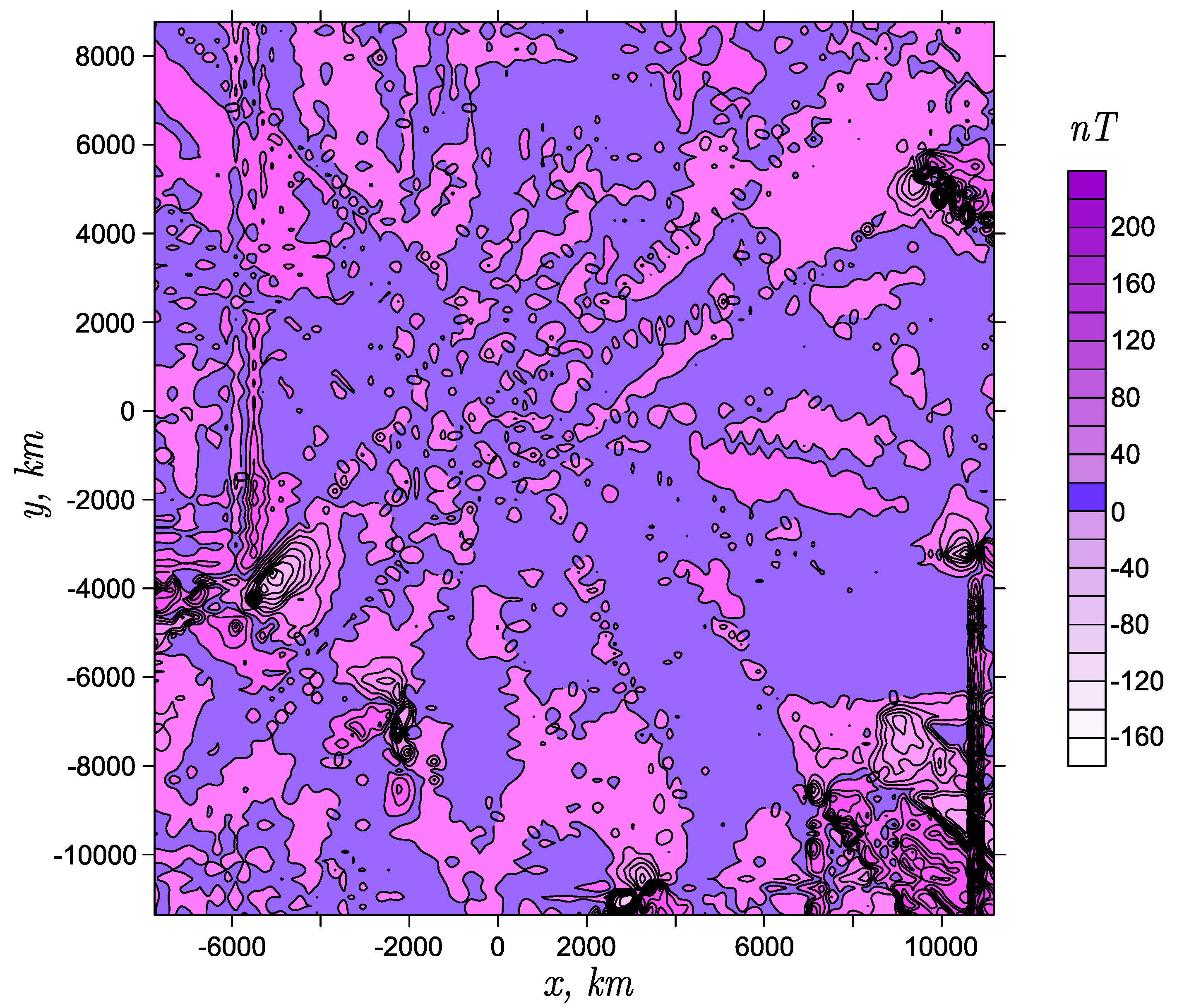
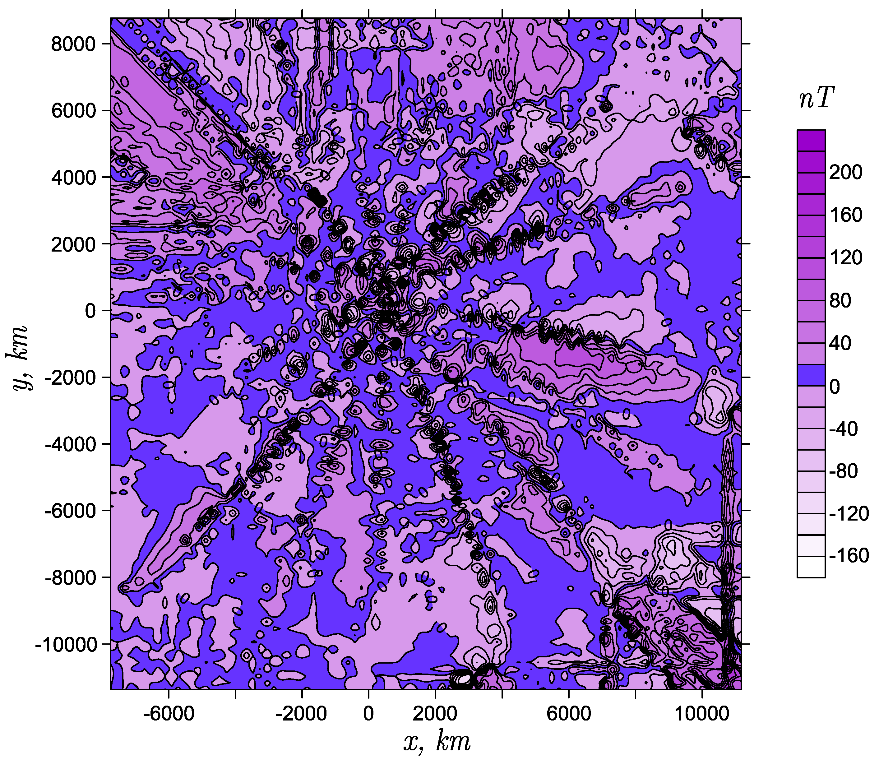
Figure 1 shows the values of the z-component of the magnetic induction vector according to measurements from the MESSENGER station. Figure 2 shows the results of regional S-approximations of the indicated component at the orbital points. The orbit of the space mission at some points in time went quite far from the surface of Mercury (at a distance of up to 0.6 of the average radius of the planet); thus, to isolate from the “raw data” the components of magnetic induction generated by currents in the liquid core and crust—the so-called Mercury’s internal magnetic field—one can use the “thin shell” approximation [15]. With this approach, the observation points must be located within the thin (compared to some parameters characterizing the topology of the planet) shell surrounding Mercury. The poloidal and toroidal magnetic fields created by currents in the plasma around Mercury “disappear” in this case. We carried out mathematical modeling of Mercury’s magnetic field based on the above-mentioned principle of a “thin shell”: each segment from a certain set of data obtained during the motion of the satellite does not extend beyond the boundaries of a spherical shell, the thickness of which is approximately 0.1 of the radius of Mercury, i.e., 240 km. The approximation of Mercury’s magnetic field is constructed as follows:

• a mathematical model of the magnetic induction vector measured along the flight paths of the MESSENGER station is constructed;
• the measurement area of “raw data” is divided into spherical layers with a thickness not exceeding 230–235 km, and in these layers the values of the components of the magnetic induction vector are found using the distributions of equivalent sources determined in the previous stage;
• analytical models of the field at arbitrary points and distributions of equivalent sources are determined from the data synthesized in the second stage.

Figure 1. Isoline map of Mercury’s magnetic field according to data from the MESSENGER mission ($B_z$-component).

Figure 1. Isoline map of Mercury’s magnetic field according to data from the MESSENGER mission ($B_z$-component).

Figure 2. Isoline map of Mercury’s magnetic field near the surface, constructed using regional S-approximations.

Figure 2. Isoline map of Mercury’s magnetic field near the surface, constructed using regional S-approximations.

In order to have 10,000 points remaining in the set for which the approximations were performed, we synthesized, so to speak, additional intermediate nodes and “attributed” to them some averaged values of the magnetic field elements. Using the found distributions of equivalent sources, we found the spatial distribution of magnetic field elements, thus continuing, or extrapolating, the approximated field to other points of the satellite orbits under consideration.

Due to the fact that the process of approximating “raw data” about the magnetic induction vector is divided into several stages, the proposed technique can be used when performing analytical continuations of fields downward, towards the sources. If the data sample does not satisfy the conditions of the “thin shell” principle, then we will obtain distributions of equivalent magnetic masses in the crust that do not correspond to reality.

Important note. Adequate mathematical models of the planet’s magnetic field are necessary to identify the conditions for the existence and unique solvability of the inverse coefficient problem for the second part of the system (2), which describes the motion of a charged fluid inside the planet (namely—finding the spatial distribution of fluid velocity components and viscosity coefficient). In this case, as can be seen from the above equation, the problem becomes more complicated, since a nonlinear inverse coefficient problem is obtained with respect to speed.

5. Conclusions

The uniqueness theorem for the solution of the inverse problem of determining the magnetic diffusion coefficient, as proven in the work, was formulated for the case of restoring the desired parameters in the entire upper half-space. In this way, the results first presented in the work [6] were generalized, in which a similar theorem was formulated for the case of recovering the sought parameters only on a certain closed bounded set. Thus, the result obtained in this work will make it possible to reduce the arbitrariness in mathematical modeling of physical processes describing the magnetic field of planets with a magneto-hydrodynamic dynamo.