Abstract
This paper proposes a graph residual gated recurrent network subway passenger flow prediction model considering the flat-peak characteristics, which firstly proposes the use of an adaptive density clustering method, which is capable of dynamically dividing the flat-peak time period of subway passenger flow. Secondly, this paper proposes graph residual gated recurrent network, which uses a graph convolutional network fused with a residual network and combined with a gated recurrent network, to simultaneously learn the temporal and spatial characteristics of passenger flow. Finally, this paper proposes to use the spatial attention mechanism to learn the spatial features around the subway stations, construct the spatial local feature components, and fully learn the spatial features around the stations to realize the local quantization of the spatial features around the subway stations. The experimental results show that the graph residual gated recurrent network considering the flat-peak characteristics can effectively improve the prediction performance of the model, and the method proposed in this paper has the highest prediction accuracy when compared with the traditional prediction model.
Keywords:
spatial attention mechanism; local character component; graph convolutional network; gate recurrent unit MSC:
68-06
1. Introduction
With the development of urbanization, the proportion of metro in urban public transportation is also growing gradually. The rapid development of the metro provides great convenience for urban residents to get around. However, due to the increasing urban population, the operational efficiency of the public transportation system has been affected to some extent. Reasonable train scheduling and passenger flow distribution can improve the operational efficiency of the metro, so this is one of the popular research directions.
In recent years, metro passenger flow forecasting has become an indispensable study in intelligent transport systems, with a focus on predicting urban rail transit passenger flow. However, there are many factors affecting metro passenger flow, making the forecast results based only on the temporal characteristics of metro passenger flow deviate significantly from the reality. For example, when subjected to external influences, the metro passenger flow will show some fluctuating and abrupt trends. Such impacts are episodic and not time-specific, and metro passenger flows can have sudden and unpredictable trends under the influence of weather and large events. This makes it more difficult to study passenger flow in urban rail transit.
In addition, the time of occurrence and duration of the morning and evening peaks vary from city to city. The morning and evening peaks in cities with longer commuting distances usually occur earlier and last longer than those in small- and medium-sized cities. The characteristics of the morning and evening peaks vary between cities, making it difficult to precisely identify the intrinsic relationship between stations and passenger flow characteristics and the duration of the morning and evening peaks. This makes it more difficult to study the spatial impacts of metro stations.
To address the above issues, there are various clustering algorithms such as distance-based clustering algorithms (K-Means [1], KNN [2]), density-based clustering algorithms (DBSCAN [3], OPTICS [4]), and so on. Since the clustering effect of a single clustering method is not significant, more and more scholars study metro passenger flow prediction. Due to the shortcomings of traditional statistical prediction models and machine learning models in learning the abrupt trend of passenger flow and the influence of external factors, there are more scholars using deep learning models for prediction. Deep learning is widely used in image [5], data mining [6], prediction [7], etc. The deep learning model is used to deeply mine the correlation features of metro passenger flow other than temporal characteristics. The main prediction algorithms include Convolutional Neural Networks (CNN) [8], Long Short-Term Memory (LSTM) [9,10], and fully connected deep neural networks (FCDNNs) [11]. CNN extracts local features with a convolution operation. This algorithm is translation invariant and can learn spatial features, but it lacks a memory mechanism and has some drawbacks in dealing with sequential data. RNN has a memory function and can handle variable-length sequence data, but its training speed is slow, resulting in poor real-time prediction. Compared to RNN, GRU is more adept at capturing long-term temporal dependencies and has a small number of parameters, reducing the risk of overfitting. However, metro passenger flow is not only affected by the time factor, but also related to the spatial factor and other external factors. The temporal characteristics of different stations will be different, especially as the change in passenger flow during peak hours will have an impact on the prediction model. Since it is difficult to accurately predict metro passenger flow by solely relying on temporal features, more and more scholars combine temporal features with spatial features for metro passenger flow prediction. For example: Zhang et al. [12] proposed a prediction model that combines Residual Networks (ResNet), Graph Convolutional Networks (GCN), and Long Short-Term Memory (LSTM) using different temporal granularities. However, the spatial correlation of metro passenger flow data is more complex than the temporal correlation, and it is more difficult to measure the extent of its impact, as well as the possible impacts of the nature of the surrounding land use, which is a difficult issue that needs to be further addressed.
In order to solve the above problems, this paper proposes a metro passenger flow prediction model for graph residual gated recurrent networks considering the flat-peak characteristics. The main contributions of this paper are reflected in the following aspects:
(1) This paper proposes an improved DBSCAN clustering method to perform density clustering on the swipe data of subway passengers, and dynamically divides the flat-peak time period of passenger flow through the density clustering method, so that the prediction model can better learn the characteristics of the passenger flow in the time, and enhance the learning of the sudden change trend of the passenger flow during the time period of the flat-peak convergence, so as to improve the prediction accuracy of the prediction model.
(2) The graph residual gated recurrent network is constructed considering the flat-peak characteristics, and the spatio-temporal characteristics of the subway passenger flow are learned using different inputs according to the results of the division of the flat-peak time period. In order to better learn the influence of the spatial characteristics around the subway stations on the changes of the passenger flow as well as on the division of the flat-peak time period, this paper proposes to use the residual network in combination with the graph convolutional network, which can fully learn the spatial and temporal characteristics of the passenger flow, thus increasing a certain depth to improve the prediction accuracy of the model.
(3) This paper uses the spatial attention module for the graph residual network. By using the spatial attention module, the spatial features within a certain range around the subway station are extracted to learn the influence of the spatial features around the station on the flow of passengers, so as to analyze the changes in the influence of different spatial features on the flow of passengers and the possible influence on the results of the dynamic division of the flat-peak time period.
The remainder of the paper is organized as follows. Firstly, we review related work in Section 2. Secondly, we built a density clustering method for metro swipe card data in Section 3. Thirdly, we present a graph residual gate recurrent network metro passenger flow prediction method considering the characteristics of flat-peak characteristics in Section 4. Fourthly, experiments and results are analyzed in Section 5 to validate the feasibility and validity of the proposed method through comparison. Lastly, conclusions and perspectives for future research work are given in Section 6.
2. Literature Review
With the development of intelligent transportation, metro passenger flow prediction has become one of the popular research directions in transportation planning and management. However, from the research of scholars at home and abroad, it can be found that metro passenger flow forecasting methods can be roughly divided into four categories: statistical theory-based forecasting models [13], machine learning-based forecasting models [14], deep learning-based forecasting models [10], and combined learning-based forecasting models [15]. In the early days, many scholars used statistical theoretical passenger flow forecasting methods by analyzing the temporal correlation of passenger flow through mathematical modeling methods, which include the exponential smoothing method [16], ARIMA [17], Chaos Theory [18], and other classic prediction methods. This type of prediction model needs to predict after getting the time correlation through learning in the prediction process, and the real-time and accuracy of its model prediction will fluctuate greatly. Therefore, there will be a large error in the practical application.
In the 1990s, machine learning became one of the hottest research fields in the computer field. Because the statistical theory model cannot be better adapted to the passenger flow, data may be due to the external environment brought about by the sudden change, and machine learning can automatically analyze from the data to obtain the pattern of change in the passenger flow and use the law of the algorithm for the prediction of future moments. There are many scholars using machine learning models for passenger flow prediction. Some of the more representative machine learning forecasting models include Decision Trees [19], Simple Bayes [20], Random Forest [21], ANN [22], KNN [23], and SVM [24,25]. Huan et al. [26] proposed an optimized KNN algorithm for passenger flow prediction, and Liu et al. [27] proposed the SVM-KNN model for predicting bus passenger flow under rainfall conditions. However, these models are more susceptible to external factors in the prediction process, resulting in a certain degree of error.
With the development of the computer field, unlike the traditional linear regression and other single-dimensional feature extraction in machine learning models, the hidden neural network in deep learning models can better explore the deeper correlation of passenger flow. Deep-learning passenger flow prediction models are mostly used for short-term passenger flow prediction. More representative models include LSTM [28,29], GRU [30,31], RNN [32], GCN [33,34,35], and other deep learning models. Wang et al. [36] proposed a spatio-temporal hypergraph convolutional model for metro passenger flow prediction. Feng et al. [37] used LSTM to predict urban rail transit passenger flow in rainy and snowy weather. CHENG proposed the use of DL-SVR [38] or prediction by combining a deep learning model with SVR. Wang et al. [39] proposed the use of convolutional long and short-term memory neural networks for rail transit passenger flow prediction, and these prediction models are improved compared to statistical theoretical models and machine learning models, but there are still some shortcomings. For example, CNN has certain spatial feature learning abilities, and LSTM and GRU can better handle the correlation of passenger flow data in time. However, the passenger flow is not only correlated in time, but also related to spatial features, and the passenger flow will be different in different stations.
Therefore, to serve the defects of a single model, many scholars have begun to use the combination model to predict the passenger flow, and these combination models can take into account the multiple characteristics of the historical data at the same time so as to make the prediction of short-term passenger flow more accurate. These combined models can effectively solve the defects of single models so as to better improve the prediction accuracy of short-term traffic flow. Zhang et al. [40] proposed to use CNN and LSTM for the combination of prediction, and the model has a certain degree of superiority and robustness. Yang et al. [41] improved the wavelet packet decomposition and combined it with LSTM, which can improve the prediction performance of the model to a certain extent. Yang et al. [42] improved the wavelet and combined it with ARMA, which can effectively improve the efficiency of the model. Xu et al. [43] used GCN and RNN for combined learning, and at the same time considered the spatial and temporal characteristics of the passenger flow. Xue et al. [44] not only used traditional metro swipe data, but also used social media data for metro flow prediction, which could improve the prediction accuracy of the model to a certain degree. Huang et al. [45] used a deep trust network combined with the MTL multitasking layer, and the model has better generalization performance. Zeng et al. [46] constructed a CEEMDAN-IPSO-LSTM combination model to predict urban rail transit passenger flow, and its prediction accuracy was significantly improved. Through the comparative analysis of several examples, such methods can effectively improve the accuracy of short-term passenger flow prediction, which is a development direction of passenger flow prediction in the future, and is also a hot spot of current research.
From the above research results, it can be found that the combination class prediction model is currently the main research direction in this field. Research on key methods is ongoing and has limitations, and several aspects warrant further investigation, as follows.
(1) Although these studies were able to pre-process the passenger flow data, the influencing factors around different stations may result in slightly different peak time periods, and the ability of the prediction model to cope with sudden changes in the data may affect the prediction accuracy to a certain extent.
(2) Since different spatial features around the station will lead to different results in the division of its flat-peak time period, some scholars propose to fully learn the spatial correlation of the metro network. As its focus is broader when learning spatial features, it is difficult to focus on learning the spatial influence within a certain range around the station, which means the prediction model cannot fully learn the spatial features of the metro stations, resulting in the poor prediction effect of the model.
This paper solves the above two problems. To address the problem of dividing the flat-peak time period of different stations, the density clustering method is used to cluster the density of passenger card swipes with the expectation of dynamically dividing the flat-peak time period of metro passenger flow. To learn the spatial influence of a certain range around the metro station in a targeted way, this paper proposes the use of a graphical residual gate recurrent network considering the flat-peak characteristics of passenger flow to learn and predict the temporal and spatial characteristics of passenger flow at the station, thus achieving a practical and real-time metro passenger flow prediction model.
3. Dynamic Division of Peak Hours
Metro passenger flow is usually affected by more factors, and the length of residents’ commuting distance will affect the duration of the urban morning and evening peak hours to a certain extent. Therefore, the morning and evening peak hours of different stations will appear at different times, the arrival of the peak hours will make the metro passenger flow generated by the sudden change, resulting in the prediction model. The prediction of the sudden change in the trend cannot be learned, and thus the model prediction accuracy, to a certain extent, is affected. At the same time, due to the different locations of metro stations and the different spatial properties of the surrounding areas, the morning and evening peak time periods of different stations are different.
Therefore, to solve the above problems, in the paper, a Density-Based Spatial Clustering of Applications with Noise (DBSAN) clustering algorithm is improved, which clusters the metro card data, and dynamically divides the morning and evening peak time slots of the target stations according to the clustering results. The DBCAN algorithm is shown below:
where D is the data set, ε is the neighborhood, and dist(p, q) is the distance between points p, q. Nε(p) is the neighborhood of p in the data set D. If point p is in the neighborhood of q and point p satisfies the condition of Equation (2), then point p is said to be reachable concerning point q with respect to ε and MinPts density. At this point, a point pi is said to be reachable concerning point q with respect to ε and MinPts density if there exists a chain of objects p1p2…pn, p1 = q, pn = p, pi ∈ D (1 ≤ i ≤ n). Points p and q are said to be density connected if there exists a point o ∈ D from which both points p and q are reachable with respect to the ε and MinPts densities. n is a point in D and Ci is one of the clusters in D. If n does not belong to any of the clusters in D, it is assumed that n is noise in the set.
Since changes in the parameters of the traditional DBSCAN algorithm can have a great impact on the classification results of the algorithm, DBSCAN is improved in the paper so that it can perform clustering more efficiently and accurately. An inverse Gaussian distribution statistical model was fitted to this probability distribution [47], and the value corresponding to the peak was determined to be ε. MinPts should not be a fixed value, and thus it is necessary to find the point i0 such that noisei0 and are approximately equal, and the intersection of the 45° straight line with the Noise curve is taken as MinPts = i0.
In metro passenger data, the swipe density is pseudo-peak during off-peak hours due to group travel, and by adding judgment conditions to the clustering results, to avoid being concluded as pseudo-peak hours. Thus, starting from any core point object, all objects reachable from the density of that object form a cluster. There are n object points in a cluster, and if more than 90% of the points in the cluster satisfy Equation (6), the cluster is recognized as an early morning and late evening peak time period based on the time period in which it is located.
4. A Prediction Model for Graph Residual Gated Recurrent Networks Considering Flat-Peak Properties
4.1. Model Construction
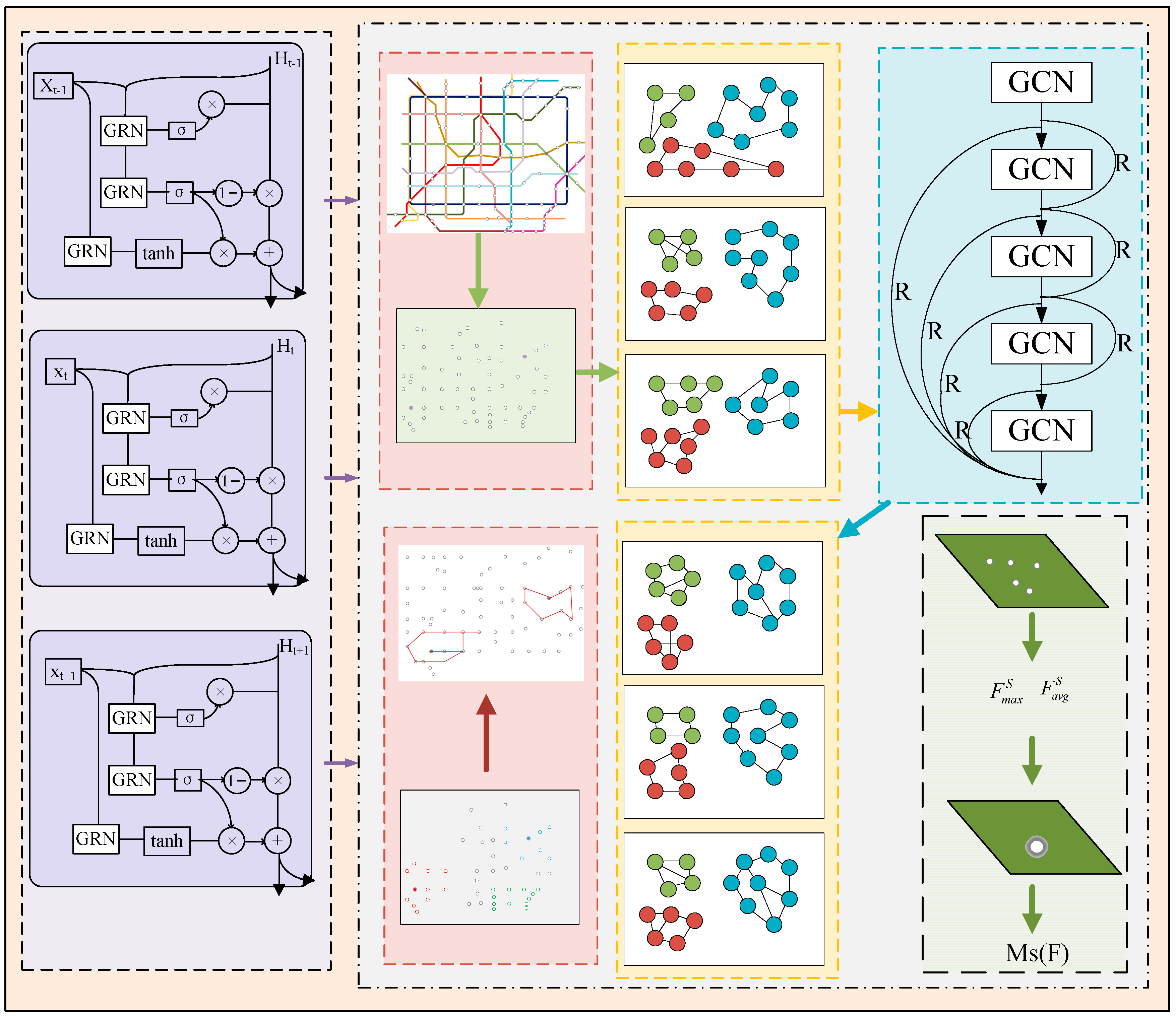
Urban metro passenger flow can be affected by more external factors, because the different travel demand leads to passengers’ choice of the travel time period being different. Travel is usually divided into rigid and flexible travel. The proportion of commuter travel generally accounts for about 80% of the total travel, belonging to the rigid travel, and there are time constraints, so that the metro passenger flow has a more obvious peak phenomenon. In addition to commuting trips, travelling outside the time constraints of the trip is called flexible travel or life travel, the proportion of about 20% of the total travel in the metro passenger flow in the performance of the peak time period. For some of the elastic travel demand, people’s travel time periods are influenced by the spatial characteristics of the site’s neighborhoods. As a result, the spatial nature of the neighborhood leads to different peak periods and durations at different stations. For the changes between the peak time period and the peak time period, there will be a large change trend, leading to the model in the prediction to find the pattern of change of passenger flow with more difficulty. To overcome this difficulty, a graphical residual gated recurrent network metro passenger flow prediction model considering the flat-peak characteristics is proposed, where the appearance and duration of passenger flow in the flat-peak time period of different stations, the trend of metro passenger flow in the flat-peak, and the influence of spatial characteristics around a station on the passenger flow at that station can be better learned. The framework of the passenger flow prediction model for the graphical residual gated recurrent network considering the flat-peak characteristics is shown in Figure 1.
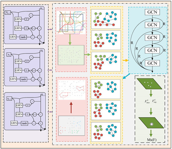
Figure 1.
Prediction Schematic of the modeling framework.
In Figure 1, xt−1, xt, xt+1 is the passenger flow at the moment t − 1, t, t + 1, respectively, R is the residual connection, GRN is the linear operation, σ is the Sigmoid activation function, Ht−1 is the hidden layer state at the moment of t − 1, and Ht is the hidden state that is passed to the next node. MS(F) is the weight of spatial attention mechanism, is the average pooling operation, and is the maximum pooling operation.
The network structure used in the paper is an undirected weighted graph G = (V, E), V is the vertex set, each underground station in the underground network. V = {V1, V2, V3, …Vn} is the number of vertices, the number of underground stations within the study area. E stands for the set of edges, the track lines in the underground network.
To better to learn the effect of stations on passenger flow and combine it with the division of peak time periods, according to the results obtained from the clustering by DBSCAN, the data is divided into peak time period and flat time periods. According to the different time periods, the data will be input into different modules of the model. In this paper, we propose to use the residual module to connect the graph convolution network and set local components in the graph convolution network to fully learn the spatial influence around the site.
where , , I ∈ RN×N is the unit matrix, A ∈ RN×N is the adjacency matrix, , Ht is the output of the t-th layer, Wt is the weight parameter matrix of the t-th layer, and σ is the Sigmoid activation function.
Since the influence of the site perimeter on the site traffic is different, the traditional spatial learning is not able to accurately learn the influence of spatial features on the change of traffic. Therefore, this paper proposes to use the spatial attention mechanism to learn the features of the spatial features within a certain range of the site perimeter in an effort to derive a spatial local component, and the model’s learning of the spatial influence is improved, which leads to the improvement of the model’s prediction accuracy.
where MS(F) is the weight of spatial attention mechanism, is the average pooling operation, is the maximum pooling operation, M is the hidden layer shared MLP, is the bias matrix, and GRN(X, A) is the local correlation output.
To better learn the temporal features of passenger flow, GRU is used for temporal feature learning, which can effectively avoid the gradient explosion problem. The structure of GRU includes an input layer, a hidden layer, and an output layer. In this paper, based on the GRU deep learning framework, the model uses the graph residual network that incorporates the spatial attention mechanism to enhance the spatial information processing ability of the algorithm, according to the dynamic division results of the flat-peak time period. Using the spatial attention mechanism proposed in this paper to carry out local feature learning, the different spatial influences around the site are divided into weights, and this local feature component is inputted into the GRU, and the calculation rules are shown in Equations (12)–(15).
where is the reset gate at time t, is the reset gate weight matrix, is the update gate at time t, is the hidden layer output at the previous moment, is the output at time t, Θ is the Hadamard product, and βr, βu, and βh are the corresponding filter parameters.
4.2. Steps in Model Prediction
By collecting the metro card swipe data, the relevant information needed for this study is extracted and the metro passenger flow is analyzed and preprocessed. The time period of the flat-peak of the passenger flow is dynamically divided by the improved DBSCAN, and the time period of the flat-peak varies from station to station. Predictions are made based on the morning and evening peaks obtained from the DBSCAN segmentation, and the data from different time periods are input into different models to learn the spatial features around the stations using the local components of the graph convolutional network. With the minimization of the loss function as the optimal objective, the experiments in the paper select the root mean square error as the loss function, as shown in Equation (16).
In the above equation, t is the number of samples, xt is the real value at moment t, is the predicted value at moment t, and N is the total amount of predicted data.
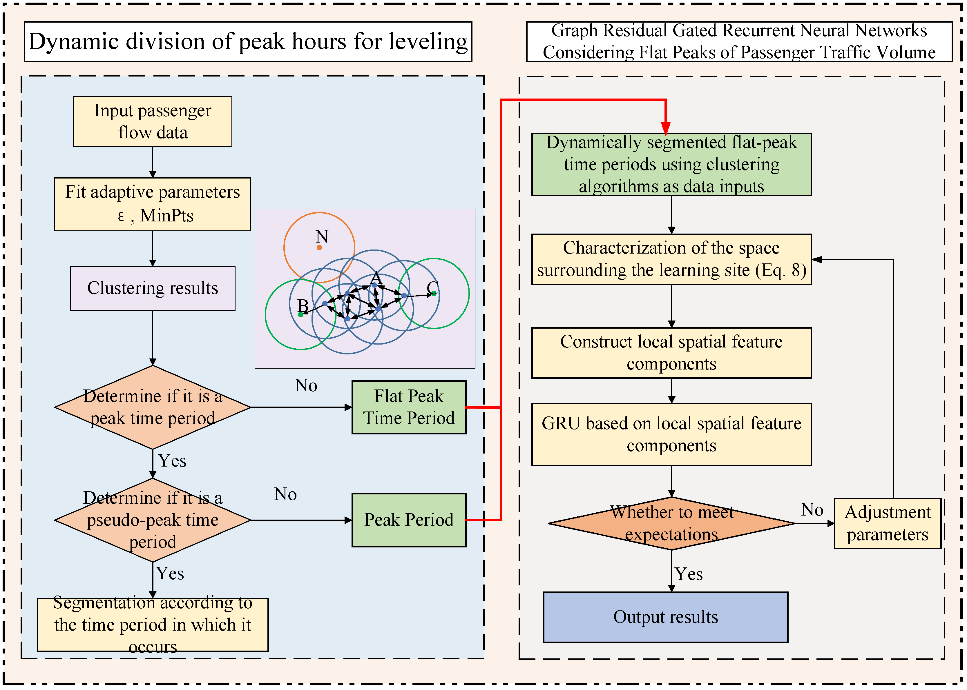
The flowchart of the metro passenger flow prediction model for the graph residual gated recurrent network proposed in this paper, which takes into account the characteristics of the level peak, is shown in Figure 2.
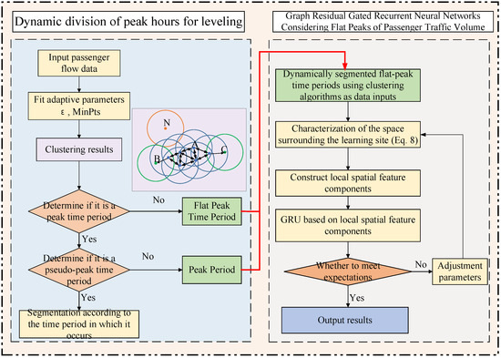
Figure 2.
Flowchart of model predictions.
In this paper, the main implementation steps of the proposed graph residual gated recurrent network metro passenger flow prediction model considering the flat-peak characteristics are as follows:
Step 1: Acquire the passenger flow data in the metro network. When collecting the passenger flow data in the metro network, the historical passenger flow time series data of the stations and the spatial characteristics around the stations are mainly collected. Pre-processing of the collected data mainly includes the processing of abnormal data and the supplementation of missing values.
Step 2: Construct an adaptive DBSCAN clustering algorithm, because the selection of parameters can lead to the clustering effect, so that through the fitting of statistical models to the data, DBSCAN can select adaptive parameters to improve the clustering effect of the algorithm.
Step 3: The flat-peak time period of passenger traffic is dynamically divided by this clustering algorithm by realizing the dynamic division of the flat-peak time period. As there will be collective travel in the metro, to avoid such conditions occurring in the time period being misjudged as the peak time period, this paper uses Equation (6) to judge it. If it meets the requirements of Equation (6), it will be judged as the peak time period.
Step 4: Construct a graph residual gate recurrent network, set up the input layer of the graph residual gated recurrent network in the flat-peak time period, the output layer of the spatial attention mechanism, and the intermediate layer of the graph residual gated recurrent network, and initially set up the structure of the explicit and implicit layers and the relevant parameters.
Step 5: The temporal and spatial characteristics of the passenger flow using n time series data dynamically classified with the DBSCAN clustering algorithm into flat-peak time segments are used as input to the model. The data are fed into different modules to better learn the effect of their spatial characteristics on passenger flow.
Step 6: Use the spatial attention mechanism to learn the spatial features around the metro station to obtain a local spatial feature component to quantify the effect of this spatial component on passenger flow. This feature component is fed into the graph residual gated recurrent network.
Step 7: Equations (13)–(15) are used to learn the temporal features of the passenger flow, combine the spatially localized feature component to learn the temporal features, pass them on, and predict the passenger flow.
Step 8: Use the training set to train the prediction model, and then use the test set to test the trained graph residual gated recurrent network metro passenger flow prediction model, and fine-tune the model parameter indexes according to the test results to further improve the prediction effect.
Step 9: Compare the prediction results with the real values, and check whether the prediction accuracy reaches the expected goal. If it meets the standard, then output the prediction results. If it does not meet the standard, then go back to step 4, adjust the model structure parameter indexes, and observe the changes in the predicted output values and evaluation indexes until the accuracy meets the expected requirements.
5. Experimental Analysis
To verify the prediction effectiveness of the clustering method and prediction model proposed in this paper, this paper carries out experiments for the Shanghai metro network through the design of relevant experiments to verify the impact of the dynamic division of the peak time period on the prediction accuracy proposed in this paper, and the prediction performance of the graph residual gated recurrent network metro passenger flow prediction model considering the characteristics of the flat peak, respectively, and to use the model of this paper to compare it with the classical prediction model.
5.1. Research Scope
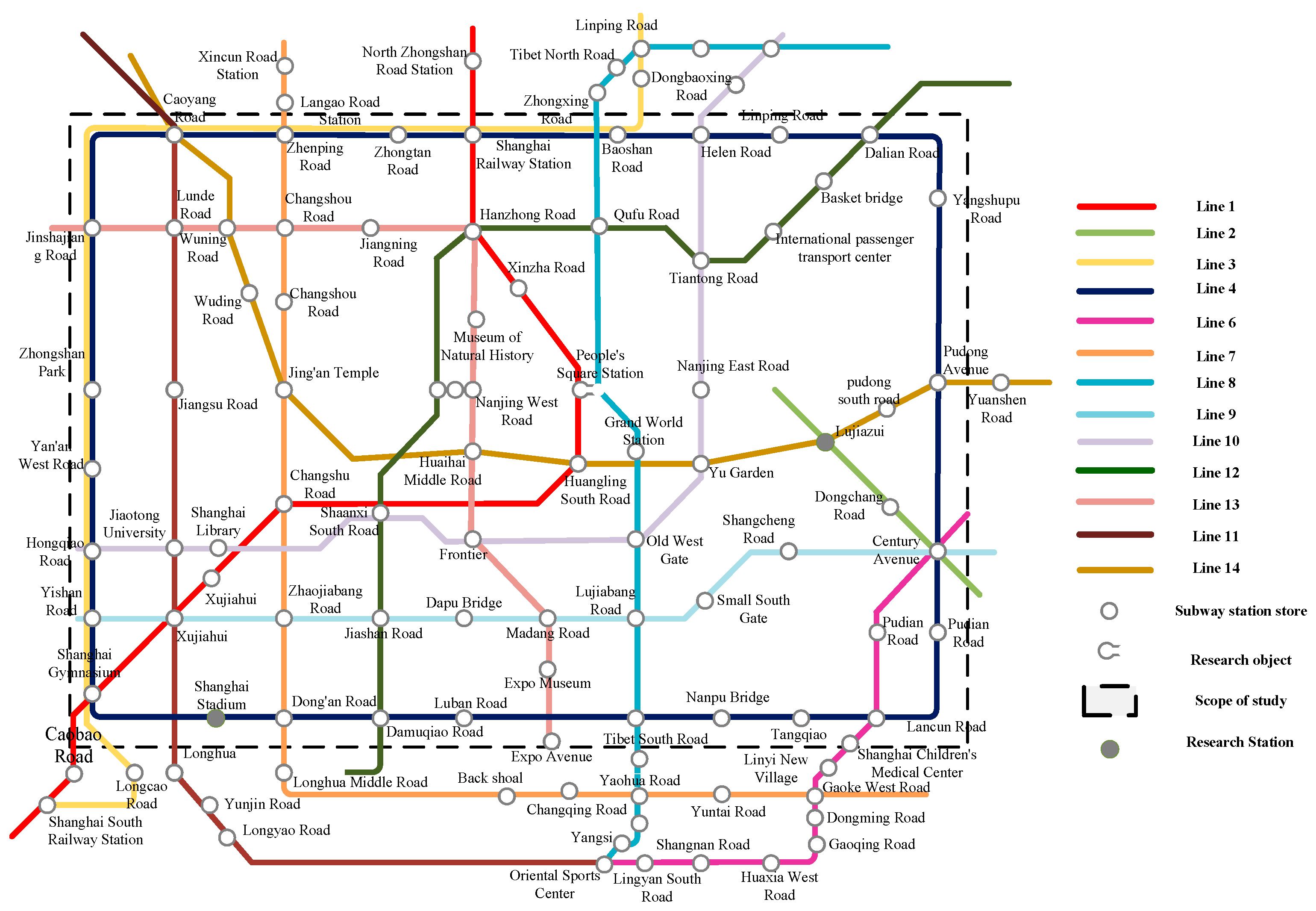
In this paper, the passenger swipe data from the Shanghai Metro network in April is used in the experiment. In this paper, Lujiazui Station and Shanghai Stadium Station are selected. Lujiazui station for line 2, line 14 is a metro transfer station, and Shanghai stadium station is in line 4 and is the metro network in the non-transfer station. Shanghai metro network distribution map is shown in Figure 3.
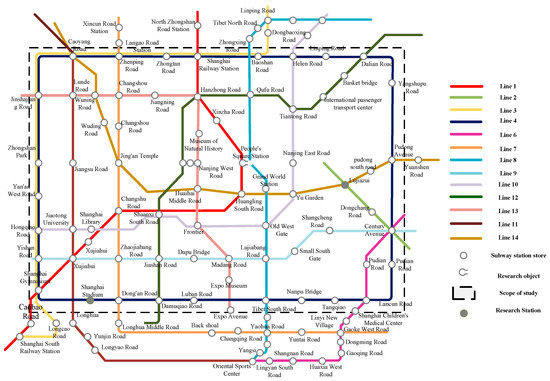
Figure 3.
Distribution of metro stations.
5.2. Selection of Indicators
To evaluate the accuracy of metro traffic flow prediction more objectively, Mean Absolute Error (MAE) [48], Mean Absolute Percentage Error (MAPE) [38], Root Mean Square Error (RMSE) [49], and Correlation Coefficient (R2) are selected as the prediction performance evaluation indexes in this paper.
where: t is the number of samples, xt is the real value at moment t, is the predicted value at moment i, is the average of the real value of passenger flow, and N is the total amount of predicted data.
5.3. Comparison of Model Improvements
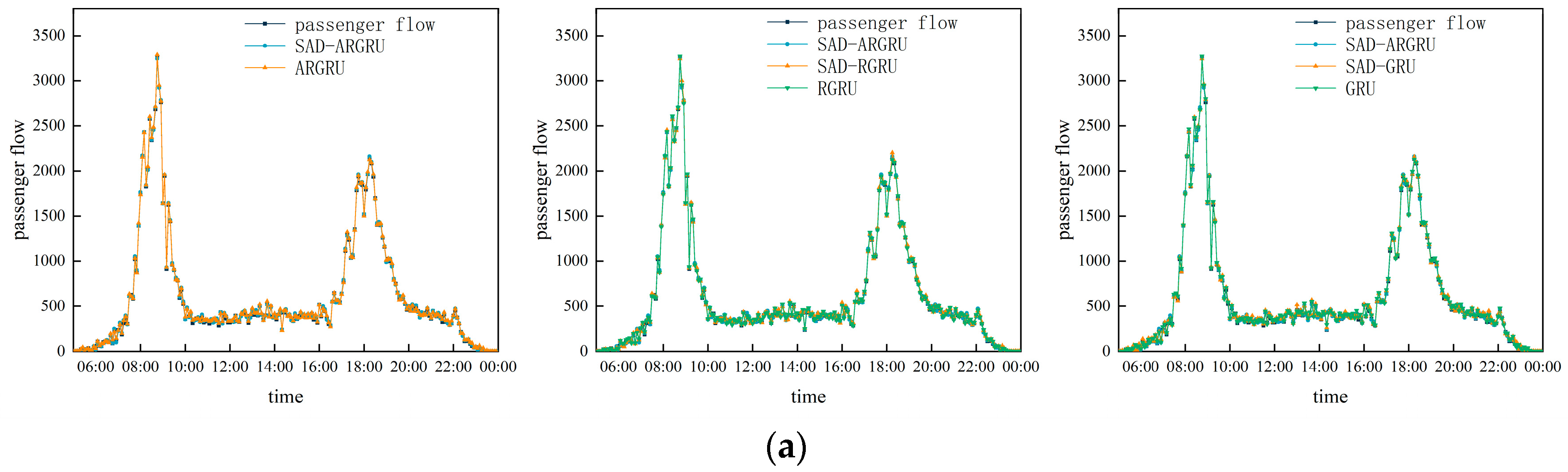
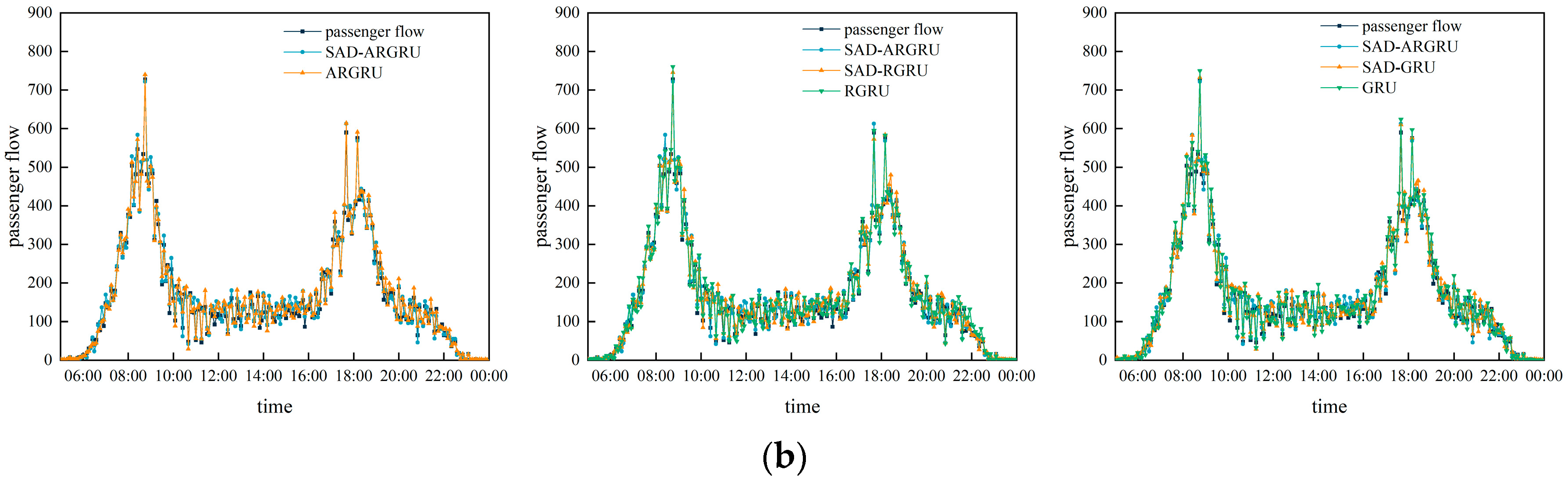
To be able to better learn the influence of metro station surroundings on passenger flow, and at the same time dynamically classify the flat-peak time period of passenger flow, we used a graph residual gated recurrent network metro passenger flow prediction model considering flat-peak characteristics (hereafter referred to as SAD-ARGRU) to evaluate the effects of the adaptive DBSCAN clustering algorithm, graph residual network, and spatial attention mechanism used in this paper on the prediction accuracy of the model. In this paper, the SAD-ARGRU, the graph residual gated recurrent network prediction model (RGRU) without spatial attention mechanism, and the traditional GRU model are used in the experiments to compare and analyze the weekend and weekday passenger flows of Shanghai Stadium and Lujiazui Station, respectively, so as to validate the effects of dynamically dividing the flat-peak time period of the flow, the graph residual network, and the spatial attention mechanism on the prediction accuracy of the model. In this experiment, the prediction performance is compared according to the evaluation indexes selected in 5.2. Figure 4 and Figure 5 show the comparison of the predicted results for the Lujiazui site and the Shanghai Stadium site on weekdays and weekends, respectively. Table 1 and Table 2 show the comparison of the evaluation indicators for the Lujiazui site and the Shanghai Stadium site on weekdays and weekends.
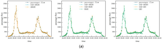
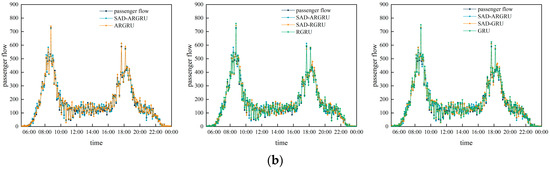
Figure 4.
Comparison results of model improvement (working days). (a) Lujiazui, (b) Shanghai Stadium.
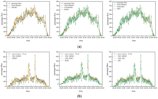
Figure 5.
Comparative results of model improvements (weekend). (a) Lujiazui, (b) Shanghai Stadium.

Table 1.
Comparative results of evaluation indicators related to model improvements (weekdays).
Table 2.
Comparative results of evaluation indicators related to model improvements (weekends).
Figure 4 and Table 1 show the results of comparing SAD-ARGRU on weekdays with the model prediction without improvement, and Figure 5 and Table 2 show the results of comparing SAD-ARGRU on weekends with the model prediction without improvement. Table 1 and Table 2 show that the prediction accuracy on weekdays is higher than that on weekends. On both weekdays and weekends, the prediction accuracy of the prediction model proposed in this paper is the highest, the graph residual gated recurrent network without using spatial attention mechanism is the second highest, and the prediction performance of the traditional GRU model is poor. It can be seen that the prediction model SAD-ARGRU proposed in this paper can effectively learn the local spatial features around the metro stations.
According to Table 1 and Table 2, it can be known that during the same weekday time period, the total daily passenger volume of Lujiazui Station is higher than that of Shanghai Stadium Station, and its prediction accuracy is higher than that of Shanghai Stadium Station. During weekends, the passenger volume of Shanghai Stadium is higher than that of Lujiazui Station, and its prediction accuracy is also higher than that of Lujiazui Station. Hence, one can see that the prediction model SAD-ARGRU proposed in this paper has a superior prediction performance in the case of larger passenger volume. As is shown in Figure 4, SAD-ARGRU’s ability to learn the trend of passenger flow during weekdays is significantly better than that of RGRU and the traditional GRU prediction model, and its ability to learn is more prominent when there is a sudden change in passenger flow. For example, on a weekday at Lujiazui station, from 7:40 to 7:45, the actual passenger flow changes from 585 to 1022, with a growth value of 437, which is nearly one time of the traffic flow, while the predicted value of SAD-ARGRU grows from 612 to 1053, with a growth value of 441, which is the smallest difference between the predicted value and the real value compared with RGRU and GRU. Among them, the MAPE of Lujiazui station on weekdays increases from 18.67 to 8.87. Therefore, the graphical residual gated recurrent network metro passenger flow prediction model proposed in this paper can effectively learn the spatial and temporal characteristics of the passenger flow to improve the prediction performance of the model to a certain extent, taking into account the characteristics of the flat peak.
5.4. Impact of Dynamic Segmentation of Peak Levelling Time Periods and Forecast Performance
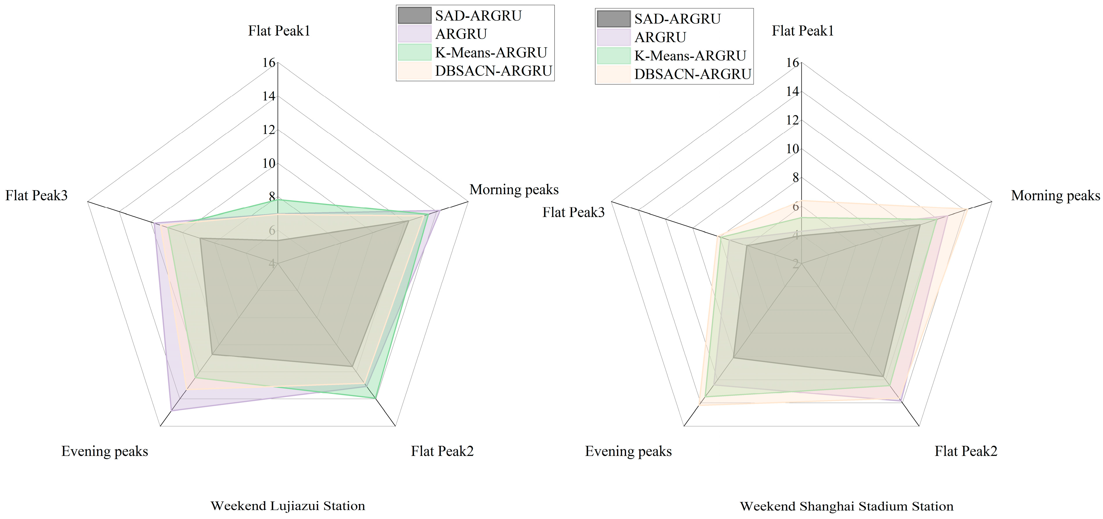
To be able to more accurately assess the impact of the adaptive DBSCAN clustering algorithm’s dynamic division of the peak level time period on the model prediction accuracy, the experiments in this paper use the adaptive DBSCAN clustering algorithm to compare with other classical clustering algorithms, and use different clustering algorithms to combine with the models in this paper, so as to compare the evaluation indexes of different combinations, in order to illustrate that the clustering algorithm proposed in this paper is useful for improving the model. In this paper, the K-Means clustering algorithm [50], and the traditional DBSCAN clustering algorithm, are selected to predict Lujiazui station and Shanghai Stadium station on weekdays and weekends, respectively, and the evaluation indexes of the prediction model are shown in Section 5.2, and the evaluation indexes of different time periods are compared on weekdays and weekends. The comparison of different time periods between weekdays and weekends is shown in Figure 6 and Figure 7. Table 3 and Table 4 show the comparison of the relevant evaluation indicators for different time periods on weekdays and weekends.
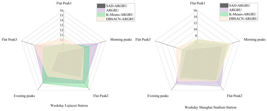
Figure 6.
Comparison of predictions of different clustering algorithms (working days).
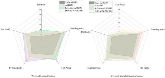
Figure 7.
Comparison of predictions of different clustering algorithms (weekends).
Table 3.
Comparison of the prediction performance of different clustering algorithms.
Table 4.
Comparative results of classical models (working day).
In Figure, Flat Peak 1 is the flat period from 5:00 am to just before the morning peak, Flat Peak 2 is the flat period between the morning and evening peaks, and Flat Peak 3 is from the evening peak to 00:00 (when the metro stops operating).
Table 3 and Figure 6 and Figure 7 show the results of the prediction comparison between Lujiazui Station and Shanghai Stadium Station on weekdays and weekends, respectively, in terms of whether they are dynamically divided into flat-peak time periods. By comparing the prediction results and related evaluation indexes, it can be seen that after using the clustering algorithm, the prediction performance of the model can be effectively improved, especially in the convergence of the flat-peak time period of the passenger flow. Through the use of clustering algorithm, it is possible to fully learn the trend of the sudden change of the flow of passengers to improve the learning ability of the model on the sudden change of the flow of passengers so as to improve the prediction performance of the model.
As can be seen from Figure 6 and Figure 7, comparing the dynamic division of flat-peak time period or not can be seen, after fully considering that the flat-peak characteristics can effectively improve the prediction performance of the model and reduce the prediction error of the model in the flat-peak convergence time period. For example, without considering the flat-peak characteristics, the MAPE of the model at Lujiazui station on weekdays is 13.45, the RMSE is 16.09, and the MAE is 13.04, while after dynamically dividing the flat-peak time period of the metro flow, the MAPE becomes 8.87, the RMSE is 14.58, and the MAE is 11.64, and the various indexes are improved to different degrees, and the MAPE is improved most obviously. MAPE is the most obvious. This is not an isolated case, as the Shanghai Stadium station on weekdays and the two stations on weekends have similar conditions. Comparing the K-Means clustering algorithm and the fisher clustering algorithm shows that the adaptive DBSCAN clustering algorithm proposed in this paper is more suitable for the prediction model proposed in this paper. In conclusion, the adaptive DBSCAN clustering algorithm proposed in this paper has a certain positive effect on the model prediction performance improvement. And its operation efficiency is also significantly higher than the traditional clustering algorithm.
5.5. Comparison of Classical Forecasting Models
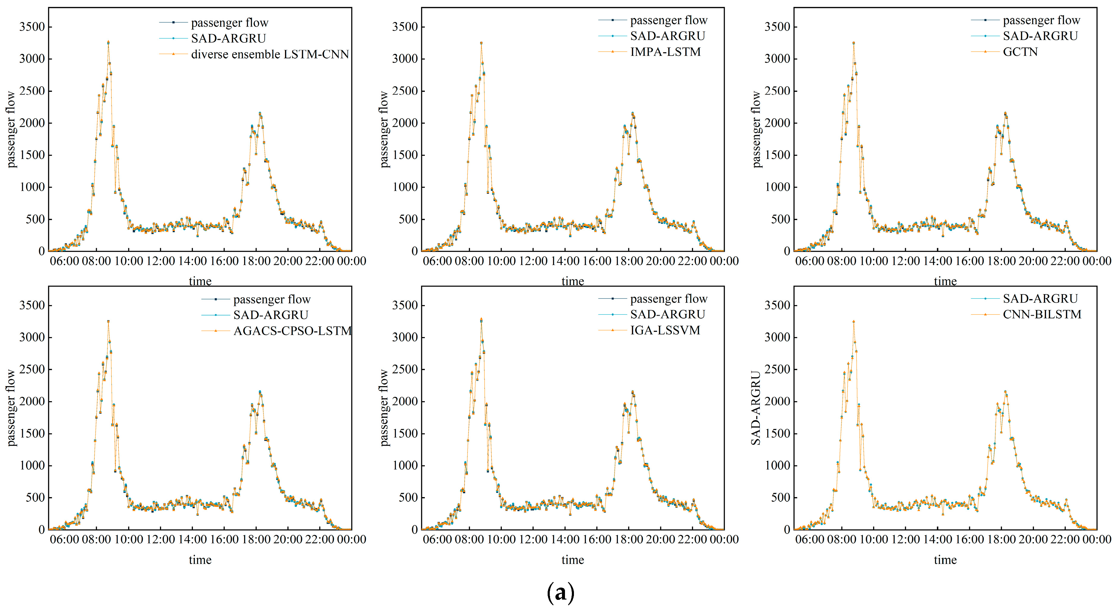
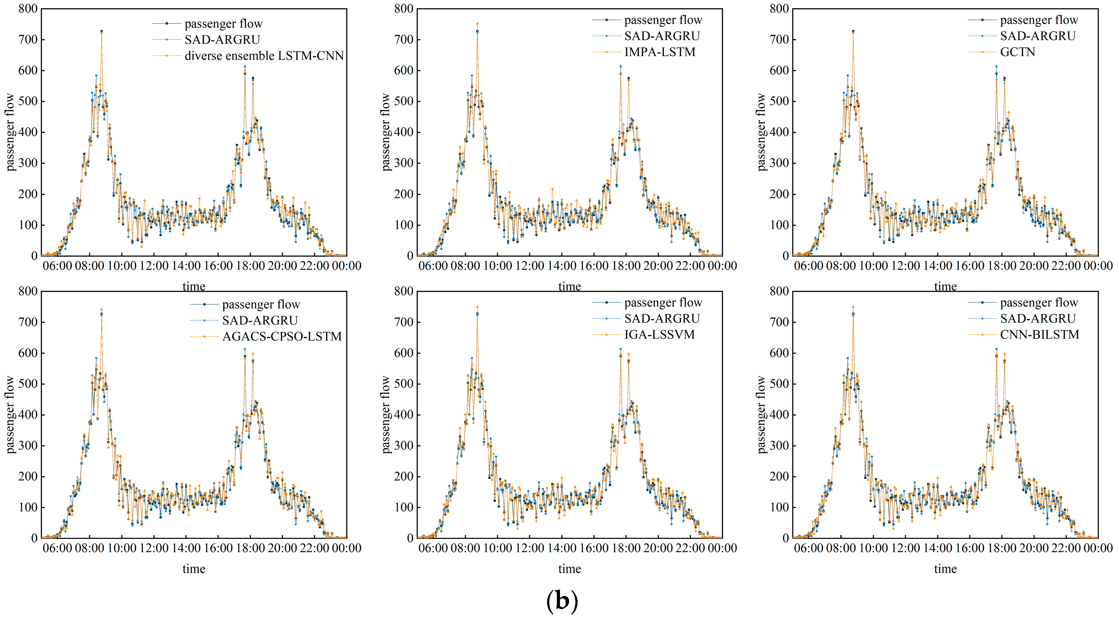
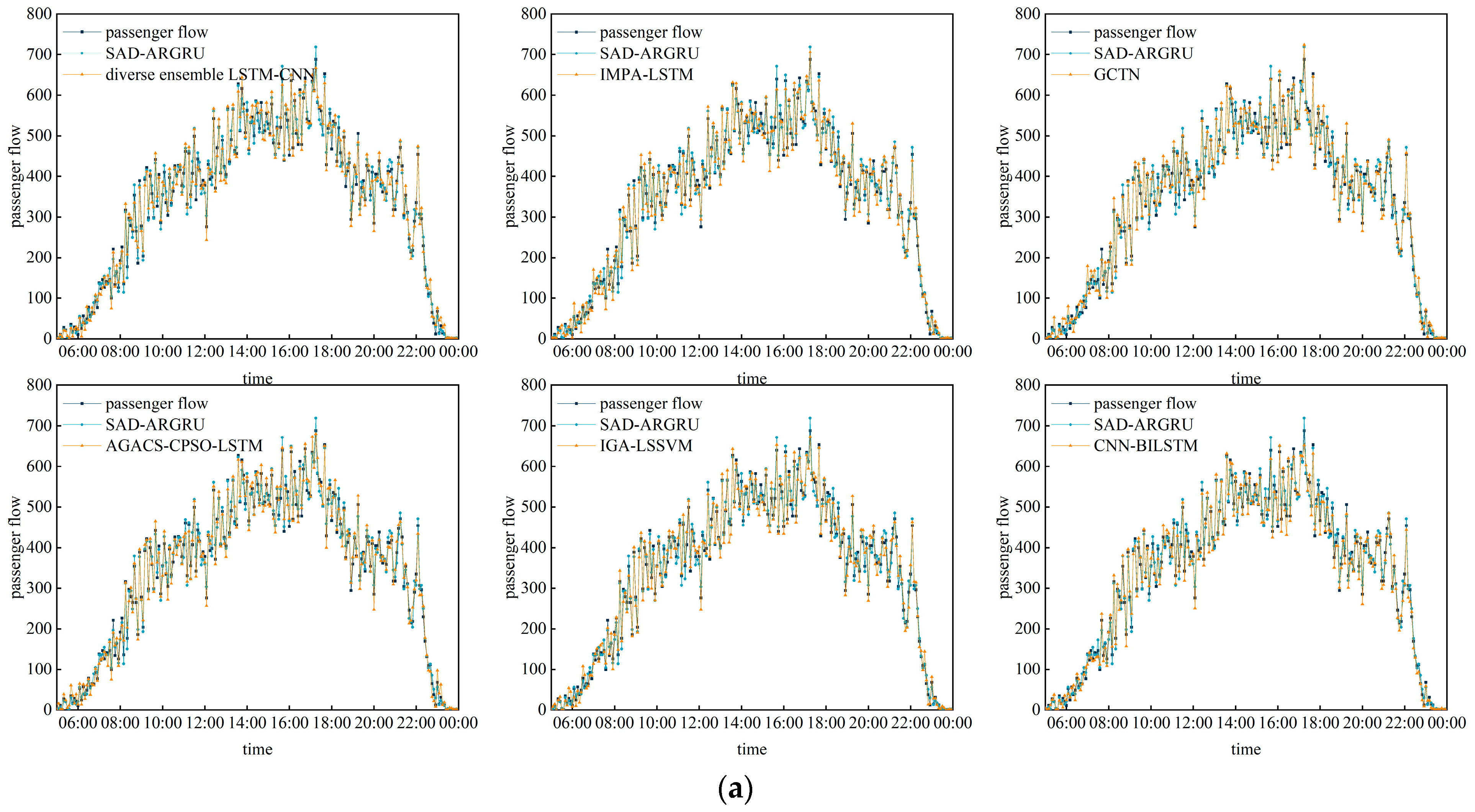
In order to be able to make a better comparison to show that the prediction performance of the proposed model in this paper has been improved compared with the classical model, eight classical prediction models were selected in this experiment to be used for the comparison with the model in this paper, which are the classical improved algorithm of LSTM and the related combined model (IMPA-LSTM [41], diverse ensemble LSTM-CNN [51], AGACS-CPSO-LSTM [52], EMD-LSTM [29]), GCN-related improved model GCTN [53]), and SVM-related improved model (IGA-LSSVM [54]). SAD-ARGRU is compared with the above classical prediction models and related improved models, and all the prediction models use the dataset selected in 5.1 with the parameter indexes selected in 5.2, and the prediction performance is compared using the evaluation indexes. In the experiment, the passenger flow prediction is carried out for Lujiazui Station and Shanghai Stadium Station on weekends and weekdays, respectively. Figure 8a,b shows the comparison of prediction results between Lujiazui Station and Shanghai Stadium Station on weekdays, and Figure 9a,b shows the comparison of prediction results between Lujiazui Station and Shanghai Stadium Station on weekends, respectively. A comparison of each evaluation index is shown in Table 4 and Table 5.
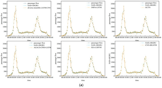
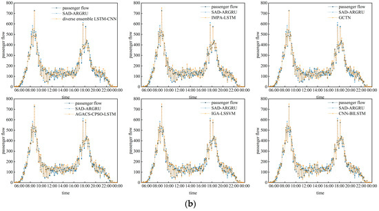
Figure 8.
Comparison with classical model predictions.(working day). (a) Lujiazui, (b) Shanghai Stadium.
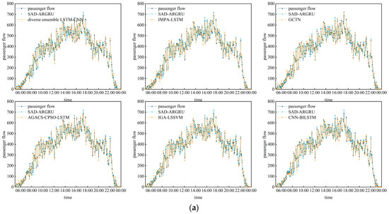
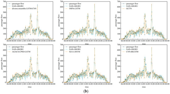
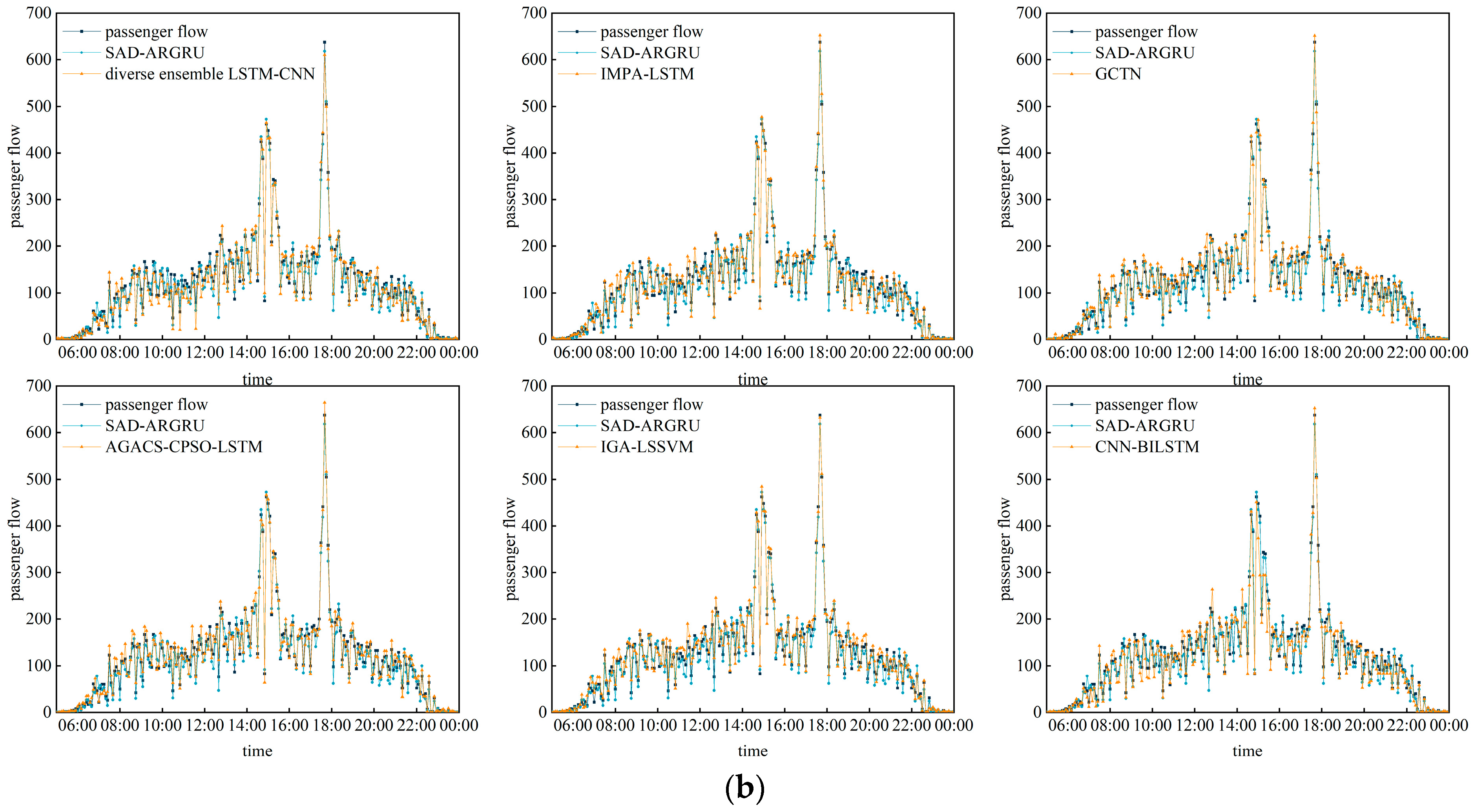
Figure 9.
Comparison with classical model predictions(weekend). (a) Lujiazui, (b) Shanghai Stadium.
Table 5.
Comparative results of classical models (weekends).
According to the above graphs, compared with the classical prediction model and the related improved model, the prediction performance of SAD-ARGRU at Shanghai Stadium station on weekends is improved more obviously, and its MAPE reduction value is about 2.87–13.04. By comparing the prediction results, it can be seen that SAD-ARGRU proposed in this paper can learn the trend of the change of the passenger flow by dynamically dividing the peak period to fully improve the prediction performance in the case of a sudden change of passenger flow. Through the spatial localization component, the spatial and temporal characteristics of passenger flow are better learned, and thus the prediction accuracy of the model is better than that of the classical passenger flow prediction model. The dynamic division of a flat-peak period proposed in this paper can effectively improve the prediction performance of the model and reduce the error between the predicted and real values of the model. For example, in Lujiazui station on weekdays, the passenger flow changes a lot in the time period between the level peaks, and in 9:20–9:25, the real value decreases from 1443 to 960, which is 66% of the previous moment, and the predicted value of SAD-ARGRU decreases from 1456 to 968, whose trend is the same as that of the real value, whereas in the classical prediction model, the error is larger.
In short-time passenger flow prediction, fully learning the spatial characteristics and the possible mutation trend of passenger flow can effectively improve the prediction performance of the model. The prediction performance of SAD-ARGRU is better than that of weekdays on weekends, and the prediction performance in Lujiazui station is even better in the same weekday situation. The changing trend of passenger flow during the weekday level-peak time period is larger, and the dynamic division of level-peak time period proposed in this paper can be predicted more accurately in the process of level-peak period convergence to improve the prediction accuracy of the model. In summary, the graph residual gated recurrent network metro passenger flow prediction model proposed in this paper considering the characteristics of the level-peak period can be more accurate in the prediction of the level-peak period convergence, and the local spatial features within a certain range around the metro station are more sufficiently learned.
6. Conclusions
In this paper, we propose a graph residual gated recurrent neural network considering the characteristics of the flat-peak passenger flow, which dynamically divides the peak period of the passenger flow by improving the DBSCAN algorithm. Due to the different travelling needs of passengers, rigid travelling needs and flexible travelling needs correspond to peak and flat-peak periods, respectively, and the dynamics of dividing the flat-peak periods can predict the trend of the passenger flow, especially in the flat-peak convergence time period. Aiming at the different characteristics of passenger flow in the flat-peak time period, this paper improves the graph convolution network to better learn the correlation between stations and analyze the influence of spatial correlation on the division of the flat-peak period. Considering the different spatial influences around the stations, this paper selects two stations with different peripheral spatial characteristics for the experiment, and the results show that the graph residual gated recurrent neural network considering the characteristics of the flat-peak passenger flow can better learn the trend of the change of the passenger flow, and the prediction value in the flat-peak articulation time period has a smaller error. Not only that, but the short-term operation can better improve the real-time prediction of the model. In the subsequent study, we will further investigate the mechanism of spatial characteristics and different station attributes on the flat-peak time period of passenger flow, as well as the characteristics of passenger flow changes between interchange stations and non-interchange stations.
By dynamically dividing the flat-peak period, the prediction model proposed in this paper is able to learn the trend of passenger flows better, thus improving the prediction accuracy of the model to a certain extent. However, for the pseudo-peaks in the flat-peak time period, the model will have some errors in the prediction process.
Author Contributions
Conceptualization, J.Z.; methodology, Y.C., S.Z. and Y.Z.; validation, J.Z., Y.C., S.Z. and Y.Z.; writing—original draft preparation, J.Z., Y.C. and Y.Z. All authors have read and agreed to the published version of the manuscript.
Funding
This research was funded by Humanities and Social Science Fund of Ministry of Education grant number 23YJAZH194.
Data Availability Statement
No new data were created or analyzed in this study. Data sharing is not applicable to this article.
Conflicts of Interest
The authors declare no conflicts of interest.
References
- He, X.; He, F.; Xu, L.; Fan, Y. Determination of the Optimal Number of Clusters in K-Means Algorithm. J. Univ. Electron. Sci. Technol. China 2022, 51, 904–912. [Google Scholar] [CrossRef]
- Zhou, Z.; Si, G.; Sun, H.; Qu, K.; Hou, W. A robust clustering algorithm based on the identification of core points and KNN kernel density estimation. Expert Syst. Appl. 2022, 195, 116573. [Google Scholar] [CrossRef]
- Hahsler, M.; Piekenbrock, M.; Doran, D. dbscan: Fast density-based clustering with R. J. Stat. Softw. 2019, 91, 1–30. [Google Scholar] [CrossRef]
- Agrawal, K.; Garg, S.; Sharma, S.; Patel, P. Development and validation of OPTICS based spatio-temporal clustering technique. Inf. Sci. 2016, 369, 388–401. [Google Scholar] [CrossRef]
- Chauhan, R.; Ghanshala, K.K.; Joshi, R. Convolutional neural network (CNN) for image detection and recognition. In Proceedings of the 2018 First International Conference on Secure Cyber Computing and Communication (ICSCCC), Jalandhar, India, 15–17 December 2018; pp. 278–282. [Google Scholar]
- Wang, S.; Cao, J.; Philip, S.Y. Deep learning for spatio-temporal data mining: A survey. IEEE Trans. Knowl. Data Eng. 2020, 34, 3681–3700. [Google Scholar] [CrossRef]
- Polson, N.G.; Sokolov, V.O. Deep learning for short-term traffic flow prediction. Transp. Res. Part C Emerg. Technol. 2017, 79, 1–17. [Google Scholar] [CrossRef]
- Zhao, J.; Shen, J.; Liu, L. Bus passenger flow classification prediction driven by CNN-GRU model and multi-source data. J. Traffic Transp. Eng. 2021, 21, 265–273. [Google Scholar] [CrossRef]
- Yang, X.; Xue, Q.; Yang, X.; Yin, H.; Qu, Y.; Li, X.; Wu, J. A novel prediction model for the inbound passenger flow of urban rail transit. Inf. Sci. 2021, 566, 347–363. [Google Scholar] [CrossRef]
- Liu, Y.; Liu, Z.; Jia, R. DeepPF: A deep learning based architecture for metro passenger flow prediction. Transp. Res. Part C Emerg. Technol. 2019, 101, 18–34. [Google Scholar] [CrossRef]
- Qu, L.; Li, W.; Li, W.; Ma, D.; Wang, Y. Daily long-term traffic flow forecasting based on a deep neural network. Expert Syst. Appl. 2019, 121, 304–312. [Google Scholar] [CrossRef]
- Zhang, J.; Chen, F.; Cui, Z.; Guo, Y.; Zhu, Y. Deep learning architecture for short-term passenger flow forecasting in urban rail transit. IEEE Trans. Intell. Transp. Syst. 2020, 22, 7004–7014. [Google Scholar] [CrossRef]
- Van Der Voort, M.; Dougherty, M.; Watson, S. Combining Kohonen maps with ARIMA time series models to forecast traffic flow. Transp. Res. Part C Emerg. Technol. 1996, 4, 307–318. [Google Scholar] [CrossRef]
- Castro-Neto, M.; Jeong, Y.-S.; Jeong, M.-K.; Han, L.D. Online-SVR for short-term traffic flow prediction under typical and atypical traffic conditions. Expert Syst. Appl. 2009, 36, 6164–6173. [Google Scholar] [CrossRef]
- Guo, W.; Xu, G.; Liu, W.; Liu, B.; Wang, Y. CNN-combined graph residual network with multilevel feature fusion for hyperspectral image classification. IET Comput. Vis. 2021, 15, 592–607. [Google Scholar] [CrossRef]
- Chi, Q.; Zhongsheng, H. Application of adaptive single-exponent smoothing for short-term traffic flow prediction. Control Theory Appl. 2012, 29, 465–469. [Google Scholar] [CrossRef]
- Wen, K.; Zhao, G.; He, B.; Ma, J.; Zhang, H. A decomposition-based forecasting method with transfer learning for railway short-term passenger flow in holidays. Expert Syst. Appl. 2022, 189, 116102. [Google Scholar] [CrossRef]
- Cheng, A.; Jiang, X.; Li, Y.; Zhang, C.; Zhu, H. Multiple sources and multiple measures based traffic flow prediction using the chaos theory and support vector regression method. Phys. A Stat. Mech. Its Appl. 2017, 466, 422–434. [Google Scholar] [CrossRef]
- Wu, W.; Xia, Y.; Jin, W. Predicting bus passenger flow and prioritizing influential factors using multi-source data: Scaled stacking gradient boosting decision trees. IEEE Trans. Intell. Transp. Syst. 2020, 22, 2510–2523. [Google Scholar] [CrossRef]
- Xu, X.; Wu, Y.; Zhang, Y. Short-term passenger flow forecasting method of rail transit under station closure considering spatio-temporal modification. J. Traffic Transp. Eng. 2021, 21, 251–264. [Google Scholar] [CrossRef]
- Liu, L.; Chen, R.-C.; Zhao, Q.; Zhu, S. Applying a multistage of input feature combination to random forest for improving MRT passenger flow prediction. J. Ambient Intell. Humaniz. Comput. 2019, 10, 4515–4532. [Google Scholar] [CrossRef]
- Chen, X.; Wu, S.; Shi, C.; Huang, Y.; Yang, Y.; Ke, R.; Zhao, J. Sensing Data Supported Traffic Flow Prediction via Denoising Schemes and ANN: A Comparison. IEEE Sens. J. 2020, 20, 14317–14328. [Google Scholar] [CrossRef]
- Lin, P.; Chen, L.; Lei, Y. Short-Term Forecasting of Subway Traffic Based on K-Nearest Neighbour Pattern Matching. J. South China Univ. Technol. 2018, 46, 50–57. [Google Scholar] [CrossRef]
- Sun, Y.; Leng, B.; Guan, W. A novel wavelet-SVM short-time passenger flow prediction in Beijing subway system. Neurocomputing 2015, 166, 109–121. [Google Scholar] [CrossRef]
- Li, M.; Li, Z.; Xu, C.; Liu, T. Short-term prediction of safety and operation impacts of lane changes in oscillations with empirical vehicle trajectories. Accid. Anal. Prev. 2020, 135, 105345. [Google Scholar] [CrossRef]
- Ning, H.; Qiao, X.; Hong-xia, Y.; En-jian, Y. Real-time Forecasting of Urban Rail Transit Ridership at the Station Level Based on improved KNN Algorithm. J. Transp. Syst. Eng. Inf. Technol. 2018, 18, 121–128. [Google Scholar] [CrossRef]
- Liu, X.; Huang, X.; Xie, B. A Model of Short-term Forecast of Passenger Flow of Buses Based on SVM-KNN under Rainy Conditions. J. Transp. Inf. Saf. 2018, 36, 117–123. [Google Scholar] [CrossRef]
- Lu, X.; Wei, W.; Fei, L.; Sirui, Y.; Kejun, L.; Ye, L. Metro passenger flow prediction considering peak data rebalance. J. Railw. Sci. Eng. 2023, 20, 1611–1623. [Google Scholar] [CrossRef]
- Zhao, Y.; Liang, X.; Jiang, X. Short-term metro passenger flow prediction based on EMD-LSTM. J. Traffic Transp. Eng. 2020, 20, 194–204. [Google Scholar] [CrossRef]
- Yu, J. Short-term airline passenger flow prediction based on the attention mechanism and gated recurrent unit model. Cogn. Comput. 2022, 14, 693–701. [Google Scholar] [CrossRef]
- Sun, P.; Boukerche, A.; Tao, Y. SSGRU: A novel hybrid stacked GRU-based traffic volume prediction approach in a road network. Comput. Commun. 2020, 160, 502–511. [Google Scholar] [CrossRef]
- He, Y.; Li, L.; Zhu, X.; Tsui, K.L. Multi-graph convolutional-recurrent neural network (MGC-RNN) for short-term forecasting of transit passenger flow. IEEE Trans. Intell. Transp. Syst. 2022, 23, 18155–18174. [Google Scholar] [CrossRef]
- Wang, J.; Zhang, Y.; Wei, Y.; Hu, Y.; Piao, X.; Yin, B. Metro passenger flow prediction via dynamic hypergraph convolution networks. IEEE Trans. Intell. Transp. Syst. 2021, 22, 7891–7903. [Google Scholar] [CrossRef]
- Huo, G.; Zhang, Y.; Wang, B.; Gao, J.; Hu, Y.; Yin, B. Hierarchical Spatio–Temporal Graph Convolutional Networks and Transformer Network for Traffic Flow Forecasting. IEEE Trans. Intell. Transp. Syst. 2023, 24, 3855–3867. [Google Scholar] [CrossRef]
- Zhao, L.; Song, Y.; Zhang, C.; Liu, Y.; Wang, P.; Lin, T.; Deng, M.; Li, H. T-GCN: A temporal graph convolutional network for traffic prediction. IEEE Trans. Intell. Transp. Syst. 2019, 21, 3848–3858. [Google Scholar] [CrossRef]
- Wang, J.; Ou, X.; Chen, J.; Tang, Z.; Liao, L. Passenger flow forecast of urban rail transit stations based on spatio-temporal hypergraph convolution model. J. Railw. Sci. Eng. 2023. [Google Scholar] [CrossRef]
- Feng, S.; Liu, H.; Li, L. Prediction model of rail transit passenger flow in rain and snow weather. J. Harbin Inst. Technol. 2022, 54, 1–6. [Google Scholar] [CrossRef]
- Fu, C.; Yang, S.; Zhang, Y. Promoted Short-term Traffic Flow Prediction Model Based on Deep Learning and Support Vector Regression, J. Transp. Syst. Eng. Inf. Technol. 2019, 19, 130–134+148. [Google Scholar] [CrossRef]
- Wang, Q.; Chen, Y.; Liu, Y. Metro short-term traffic flow prediction with ConvLSTM. Control. Decis. 2021, 36, 2760–2770. [Google Scholar] [CrossRef]
- Zhang, J.; Chen, Y.; Panchamy Krishnakumari Jin, G.; Wang, C.; Yang, L. Attention-based Multi-step Short-term Passenger Flow Spatial-temporal Integrated Prediction Model in URT Systems. J. Geo-Inf. Sci. 2023, 25, 698–713. [Google Scholar] [CrossRef]
- Zhang, Y.; Yang, S.; Xin, D. Short-term Traffic Flow Forecast Based on lmproved Wavelet Packet and Long Short-term Memory Combination Model. J. Transp. Syst. Eng. Inf. Technol. 2020, 20, 204–210. [Google Scholar] [CrossRef]
- Yang, J.; Zhu, J.; Liu, B.; Feng, C.; Zhang, H. Short-term Passenger Flow Prediction for Urban Railway Transit Based on Combined Model. J. Transp. Syst. Eng. Inf. Technol. 2019, 19, 119–125. [Google Scholar] [CrossRef]
- Xu, Z.; Hou, L.; Zhang, Y.; Zhang, J. Passenger Flow Prediction of Scenic Spot Using a GCN–RNN Model. Sustainability 2022, 14, 3295. [Google Scholar] [CrossRef]
- Xue, G.; Liu, S.; Ren, L.; Ma, Y.; Gong, D. Forecasting the subway passenger flow under event occurrences with multivariate disturbances. Expert Syst. Appl. 2022, 188, 116057. [Google Scholar] [CrossRef]
- Huang, W.; Song, G.; Hong, H.; Xie, K. Deep architecture for traffic flow prediction: Deep belief networks with multitask learning. IEEE Trans. Intell. Transp. Syst. 2014, 15, 2191–2201. [Google Scholar] [CrossRef]
- Zeng, L.; Li, Z.; Yang, J.; Xu, X. Short-term passenger flow prediction method of urban rail transit based on CEEMDAN-IPSO-LSTM. J. Railw. Sci. Eng. 2023, 20, 3273–3286. [Google Scholar] [CrossRef]
- Xia, L.; Jing, J. SA-DBSCAN:A self-adaptive density-based clustering algorithm. J. Univ. Chin. Acad. Sci. 2009, 26, 530–538. [Google Scholar] [CrossRef]
- Liang, Q.; Xu, X.; Liu, L. Data-Driven Short-Term Passenger Flow Prediction Model for Urban Rail Transit. China Railw. Sci. 2020, 4, 153–162. [Google Scholar] [CrossRef]
- Liu, L.; Chen, R.-C. A novel passenger flow prediction model using deep learning methods. Transp. Res. Part C Emerg. Technol. 2017, 84, 74–91. [Google Scholar] [CrossRef]
- Meng, Y.; Liang, J.; Cao, F.; He, Y. A new distance with derivative information for functional k-means clustering algorithm. Inf. Sci. 2018, 463, 166–185. [Google Scholar] [CrossRef]
- Zhang, Y.; Xin, D. A Diverse Ensemble Deep Learning Method for Short-Term Traffic Flow Prediction Based on Spatiotemporal Correlations. IEEE Trans. Intell. Transp. Syst. 2022, 23, 16715–16727. [Google Scholar] [CrossRef]
- Zhang, Y.; Xin, D. Dynamic optimization long short-term memory model based on data preprocessing for short-term traffic flow prediction. IEEE Access 2020, 8, 91510–91520. [Google Scholar] [CrossRef]
- Zhang, Z.; Han, Y.; Peng, T.; Li, Z.; Chen, G. A comprehensive spatio-temporal model for subway passenger flow prediction. ISPRS Int. J. Geo-Inf. 2022, 11, 341. [Google Scholar] [CrossRef]
- Tan, Y.; Wu, X.; Liu, H. The Short-Term Passenger Flow Prediction of LSSVM Based on IGA. Comput. Simul. 2022, 39, 169–172+252. [Google Scholar]


Disclaimer/Publisher’s Note: The statements, opinions and data contained in all publications are solely those of the individual author(s) and contributor(s) and not of MDPI and/or the editor(s). MDPI and/or the editor(s) disclaim responsibility for any injury to people or property resulting from any ideas, methods, instructions or products referred to in the content. |
© 2024 by the authors. Licensee MDPI, Basel, Switzerland. This article is an open access article distributed under the terms and conditions of the Creative Commons Attribution (CC BY) license (https://creativecommons.org/licenses/by/4.0/).