Temporal High-Order Accurate Numerical Scheme for the Landau–Lifshitz–Gilbert Equation

Abstract

In this paper, a family of temporal high-order accurate numerical schemes for the Landau–Lifshitz–Gilbert (LLG) equation is proposed. The proposed schemes are developed utilizing the Gauss–Legendre quadrature method, enabling them to achieve arbitrary high-order time discretization. Furthermore, the geometrical properties of the LLG equation, such as the preservation of constant magnetization magnitude and the Lyapunov structure, are investigated based on the proposed discrete schemes. It is demonstrated that the magnetization magnitude remains constant with an error of $(2p+3)$ order in time when utilizing a $(2p+2)$th-order discrete scheme. Additionally, the preservation of the Lyapunov structure is achieved with a second-order error in the temporal step size. Numerical experiments and simulations effectively verify the performance of our proposed algorithm and validate our theoretical analysis.

1. Introduction

Research on micromagnetism in nanoscale ferromagnetic bodies is crucial from both scientific and technological perspectives. Currently, the exponential demand for efficient storage and processing of large-scale data has led to the emergence of magnetization dynamics and relaxation as prominent areas of research. This field encompasses various applications in the modern magnetic storage industry, such as hard-disk magnetic recording materials, magnetic reading sensors [1,2], and magnetic RAM elements [3,4]. The Landau–Lifshitz–Gilbert (LLG) equation is a fundamental equation employed in magnetization dynamics that characterizes the precessional motion of magnetization in microscale and nanoscale magnetic systems. The LLG equation exhibits two fundamental geometrical properties within magnetization dynamics. Firstly, it guarantees the unconditional preservation of magnetization magnitude, implying that magnetization magnitude remains constant throughout time and space. Secondly, it possesses a Lyapunov structure, ensuring that the system converges towards stable equilibrium states as minimum free energy when a constant external fields is applied.

The nonlinearity of the LLG equation causes significant challenges for obtaining analytical solutions, while the analytical solution can only be obtained in very few specific cases [5,6,7,8,9]. For more general cases, numerical methods are the prevalent resolution for studying magnetization dynamics. In terms of spatial discretization, researchers commonly employ finite difference methods [10,11], finite element methods [12,13], and other techniques to discretize the LLG equation. In terms of time discretization, general methods include explicit methods and implicit methods, such as the Euler method, the implicit Euler method [14], the linear multistep methods (e.g., Adams–Bashforth, Adams–Moulton, Crank–Nicholson, backward differentiation formulas (BDF)), the Runge–Kutta methods [11], etc. [15]. However, the discussion regarding the geometric properties of the LLG equation remains insufficient among the aforementioned methods. In order to preserve the inherent geometrical properties of LLG dynamics, it is crucial to focus more on suitable geometrical integrators. Numerous methods, including the Lie-group methods [16], the Gauss–Seidel projection method [17,18], the Cayley transform [19], the geometric integration on spheres [20], the mid-point rule [21,22], etc. [23,24], have been examined to develop the numerical integrators for the LLG equation. Among these techniques, the second-order accurate mid-point rule has garnered substantial popularity and widespread adoption owing to its inherent advantages in preserving the geometric properties of the LLG equation [22,23,25,26,27]. D’Aquino, Serpico, and Miano demonstrated in [21] that the mid-point rule time-stepping technique preserves the two fundamental geometrical properties of the LLG equation exactly. However, the mid-point rule is limited to second-order accuracy in time and necessitates the solution of a large discrete system comprising coupled nonlinear equations. Recently, a study investigated the two fundamental geometric properties of the LLG equation using a range of multistep discrete schemes [28]. The research revealed that a high-order multistep discrete scheme leads to better preservation of the constant magnetization magnitude, as supported by both theoretical and numerical results. Several high-order accurate methods are worth mentioning, as discussed in [29,30]. However, there is still potential to develop high-accuracy numerical schemes preserving some geometrical properties of the LLG equation.

In this paper, we propose a novel discrete scheme based on Gauss–Legendre quadrature for solving the LLG equation and analyze two fundamental geometric properties within the proposed scheme. Thanks to the high precision of the Gauss–Legendre quadrature formula, we can easily construct a high-order discrete scheme for the LLG equation. More precisely, we can achieve a $(2p+2)$th-order discrete scheme by employing $(p+1)$ Gauss–Legendre quadrature points. Additionally, we demonstrate that the magnetization magnitude is preserved with a $(2p+3)$th-order error of the temporal step size when employing $(p+1)$ Gauss–Legendre quadrature points. It can also be proven that the preservation of the Lyapunov structure is achieved with a second-order error of temporal step size.

The structure of the rest of this paper is as follows. In Section 2, we introduce the LLG equation and propose a discrete scheme based on the Gauss–Legendre quadrature. In Section 3, we analyze the property of norm preservation within the proposed discrete scheme, which effectively preserves the norm of magnetization vectors with a high degree of accuracy. In Section 4, we analyze the preservation of Lyapunov structure within the proposed discrete scheme. In Section 5, several numerical experiments are presented to validate the efficiency of our discrete scheme.

2. The Physical Model and Numerical Method

In this section we introduce the LLG equation, which describes the micromagnetic dynamic model, and propose a numerical method based on the Gauss–Legendre quadrature formulas. Furthermore, we provide a demonstration of the accuracy of the proposed numerical method.

2.1. Landau–Lifshitz–Gilbert Equation

The evolution of the magnetization vector field $\mathit{M}(\mathit{r},t)$, a function of the position $\mathit{r}\in \Omega$ and time t in a ferromagnetic body $\Omega \subset {\mathbb{R}}^3$, is described by the Landau–Lifshitz (LL) equation:

$$\frac{\partial \mathit{M}}{\partial t}=-\frac{\gamma }{1+{\alpha }^2}\mathit{M}\times {\mathit{H}}_{\mathrm{eff}}-\frac{\gamma \alpha }{M_s(1+{\alpha }^2)}\mathit{M}\times \mathit{M}\times {\mathit{H}}_{\mathrm{eff}},$$

(1)

where $\gamma$ is the absolute value of the gyromagnetic ratio, $M_s$ is the saturation magnetization, $\alpha$ is the dimensionless damping coefficient, ${\mathit{H}}_{\mathrm{eff}}$ is the effective field, which can be defined by ${\mathit{H}}_{\mathrm{eff}}=-\delta G\left(\mathit{M}\right)/\delta \mathit{M}$, and $G\left(\mathit{M}\right)$ is the micromagnetic free energy.

To account for the phenomenological damping, Gilbert introduced a damping term in reference [31] and proposed the LLG equation:

$$\frac{\partial \mathit{M}}{\partial t}=-\gamma \mathit{M}\times \left({\mathit{H}}_{\mathrm{eff}}-\frac{\alpha }{\gamma M_s}\frac{\partial \mathit{M}}{\partial t}\right),$$

(2)

which is mathematically equivalent to the LL Equation (1).

For convenience of the analysis, the dimensionless form of the LLG equation being an initial-boundary value problem is commonly used and can be expressed as

$$\frac{\partial \mathit{m}}{\partial t}=-\mathit{m}\times \left({\mathit{H}}_{\mathrm{eff}}-\alpha \frac{\partial \mathit{m}}{\partial t}\right),$$

(3)

with the homogeneous Neumann boundary condition

$$\frac{\partial \mathit{m}}{\partial \mathit{n}}{|}_{\partial \Omega }=\mathbf{0},$$

(4)

where $\mathit{m}(\mathit{r},t)=\mathit{M}(\mathit{r},t)/M_s$, ${\mathit{h}}_{\mathrm{eff}}=-\delta g\left(\mathit{m}\right)/\delta \mathit{m}$ represents the normalized effective field, $g\left(\mathit{m}\right)$ is the normalized micromagnetic free energy, and $\mathit{n}$ is the unit outward normal vector on the boundary $\partial \Omega$. The existence of a solution to the LLG equation can be found in section 4.1 of [32].

Here, the free energy $g\left(\mathit{m}\right)$ consists of normalized exchange energy, anisotropy energy, stray field energy, and external energy, given by

$$g\left(\mathit{m}\right)=\frac{C_{ex}}{{\mu }_0{M}_s^2}{\int }_{\Omega }{|\nabla \mathit{m}|}^2\mathrm{d}\mathit{x}+\frac{K_u}{{\mu }_0{M}_s^2}{\int }_{\Omega }\left(1-{\left(\mathit{m}·{\mathbf{e}}_{an}\right)}^2\right)\mathrm{d}\mathit{x}-\frac{1}{2}{\int }_{\Omega }\mathit{m}·{\mathit{h}}_s\mathrm{d}\mathit{x}-{\int }_{\Omega }\mathit{m}·{\mathit{h}}_e\mathrm{d}\mathit{x},$$

(5)

where $C_{ex}$ is the exchange constant, $K_u$ is the uniaxial anisotropy constant, ${\mathit{e}}_{an}$ is the easy axis unit vector, ${\mu }_0$ is the magnetic permeability of vacuum, ${\mathit{h}}_s$ is the stray field, and ${\mathit{h}}_e$ is the external vector field.

In the following analysis, we assume the external field to be zero. Consequently, the normalized effective field can be expressed as

$$\begin{array}{c}\hfill {\mathit{h}}_{\mathrm{eff}}=\frac{2C_{ex}}{{\mu }_0{M}_s^2}\Delta \mathit{m}+\frac{2K_u}{{\mu }_0{M}_s^2}{\mathit{e}}_{an}\left(\mathit{m}·{\mathit{e}}_{an}\right)+{\mathit{h}}_s.\end{array}$$

(6)

2.2. Numerical Method Based on Gauss–Legendre Quadrature

According to the Gauss–Legendre quadrature formulas [33], there exists a set of Gauss–Legendre quadrature weights ${\left\{{\overline{\omega }}_i\right\}}_{i=0}^p$ and Gauss–Legendre quadrature nodes ${\left\{\overline{a_i}\right\}}_{i=0}^p$ on $[-1,1]$. The following equations hold (more details are referred to Theorem 3.5 in reference [34]):

$$\left\{\begin{array}{cc}\sum _{i=0}^p{\overline{\omega }}_i{\left({\overline{a}}_i\right)}^j={\int }_{-1}^1{x}^j\mathrm{d}x=0,\hfill & \hfill \mathrm{for}\mathrm{odd}j\mathrm{with}0\le j\le 2p+1,\\ \sum _{i=0}^p{\overline{\omega }}_i{\left({\overline{a}}_i\right)}^j={\int }_{-1}^1{x}^j\mathrm{d}x=\frac{2}{j+1},\hfill & \hfill \mathrm{for}\mathrm{even}j\mathrm{with}0\le j\le 2p+1.\end{array}\right.$$

(7)

By rescaling and translation, we can obtain a set of Gauss–Legendre quadrature nodes ${\left\{a_i\right\}}_{i=0}^p$ and weights ${\left\{{\omega }_i\right\}}_{i=0}^p$ on $[0,1]$ corresponding to those on $[-1,1]$. These two sets of Gauss–Legendre quadrature nodes and weights satisfy the following equation:

$$\begin{array}{c}\hfill {\overline{a}}_i=2a_i,{\overline{\omega }}_i=2{\omega }_i.\end{array}$$

(8)

From Equations (7) and (8), we have

$$\left\{\begin{array}{cc}\sum _{i=0}^p{\omega }_i{a}_i^j=0,\hfill & \hfill \mathrm{for}\mathrm{odd}j\mathrm{with}0\le j\le 2p+1,\\ \sum _{i=0}^p{\omega }_i{a}_i^j=\frac{1}{(j+1)2^j},\hfill & \hfill \mathrm{for}\mathrm{even}j\mathrm{with}0\le j\le 2p+1.\end{array}\right.$$

(9)

We denote

$$B_j:=\sum _{i=0}^p{\omega }_i{a}_i^j,$$

(10)

and then it is obtained that, for $0\le j\le 2p+1$,

$$B_j=0,\mathrm{i}\mathrm{f} j \mathrm{i}\mathrm{s} \mathrm{o}\mathrm{d}\mathrm{d},\mathrm{and}{B}_j=\frac{1}{(j+1)2^j},\mathrm{i}\mathrm{f} j \mathrm{i}\mathrm{s} \mathrm{e}\mathrm{v}\mathrm{e}\mathrm{n}.$$

(11)

For simplicity, we introduce some notations:

$$\begin{array}{c}\hfill \mathit{D}:={\mathit{h}}_{\mathrm{eff}}-\alpha \frac{\partial \mathit{m}}{\partial t},{\overline{t}}_n:=t_n+\frac{\Delta t}{2},\end{array}$$

(12)

where $\Delta t$ is the temporal step size and $t_n=n\Delta t$.

Based on $p+1$ Gauss–Legendre quadrature nodes ${\left\{a_i\right\}}_{i=0}^p$ and weights ${\left\{{\omega }_i\right\}}_{i=0}^p$ on $[0,1]$, the general temporal discrete scheme of Equation (3) is proposed as follows:

$$\frac{{\mathit{m}}^{n+1}-{\mathit{m}}^n}{\Delta t}=-\sum _{i=0}^p{\omega }_i\mathit{m}\left({\overline{t}}_n+a_i\Delta t\right)\times \mathit{D}\left({\overline{t}}_n+a_i\Delta t\right),$$

(13)

where ${\mathit{m}}^n$ denotes the magnetization $\mathit{m}$ at time $t_n$.

Especially when $p=1$, there exists a set of according Gauss–Legendre quadrature weights and nodes ${\omega }_{\pm 1}=1/2,a_{\pm 1}=\pm 1/\left(2\sqrt{3}\right)$, and we can obtain the following two-point Gauss–Legendre discrete scheme from the general temporal discrete scheme (13):

$$\frac{{\mathit{m}}^{n+1}-{\mathit{m}}^n}{\Delta t}=-\frac{1}{2}\mathit{m}\left({\overline{t}}_n-\frac{\Delta t}{2\sqrt{3}}\right)\times \mathit{D}\left({\overline{t}}_n-\frac{\Delta t}{2\sqrt{3}}\right)-\frac{1}{2}\mathit{m}\left({\overline{t}}_n+\frac{\Delta t}{2\sqrt{3}}\right)\times \mathit{D}\left({\overline{t}}_n+\frac{\Delta t}{2\sqrt{3}}\right).$$

(14)

Remark 1. 

While $\mathit{m}$ and $\mathit{D}$ in Equations (13) and (14) have not been fully discretized, the numerical experiment should be conducted using fully discrete versions of $\mathit{m}$ and $\mathit{D}$ (please refer to Section 5 for more details). Additionally, the analysis of the two geometrical properties will be demonstrated using partially discretized versions of $\mathit{m}$ and $\mathit{D}$, rather than fully discrete ones.

For convenience, we denote $S_{\mathit{m}\times \mathit{D}}$ as

$$S_{\mathit{m}\times \mathit{D}}:=-\sum _{i=0}^p{\omega }_i\mathit{m}\left({\overline{t}}_n+a_i\Delta t\right)\times \mathit{D}\left({\overline{t}}_n+a_i\Delta t\right).$$

To show the order of the discrete scheme (13), we introduce some preliminaries first.

By Taylor series, for any $c\in \mathbb{R}$, we have

$$\begin{array}{c}\hfill \mathit{m}\left({\overline{t}}_n+c\Delta t\right)=\sum _{j=0}^{\infty }\frac{1}{j!}{\left(c\Delta t\right)}^j·{\overline{\mathit{m}}}^{\left(j\right)},\end{array}$$

(15)

$$\begin{array}{c}\hfill \mathit{D}\left({\overline{t}}_n+c\Delta t\right)=\sum _{j=0}^{\infty }\frac{1}{j!}{\left(c\Delta t\right)}^j·{\overline{\mathit{D}}}^{\left(j\right)},\end{array}$$

(16)

where $\overline{\mathit{m}}:=\mathit{m}(\mathit{x},{\overline{t}}_n)$, $\overline{\mathit{D}}:=\mathit{D}(\mathit{x},{\overline{t}}_n)$, and ${\mathit{m}}^{\left(j\right)}$ and ${\mathit{D}}^{\left(j\right)}$ denote the jth-order derivative of $\mathit{m}$ and $\mathit{D}$, respectively, with respect to time t.

Taking $t={\overline{t}}_n$ in Equation (3), it is easy to see that

$${\overline{\mathit{m}}}_t=-\overline{\mathit{m}}\times \overline{\mathit{D}},$$

(17)

where ${\overline{\mathit{m}}}_t$ denotes the first-order derivative of $\overline{\mathit{m}}$ with respect to time t.

By differentiating both sides of Equation (17), we obtain, for any positive integer s,

$${\overline{\mathit{m}}}^{(s+1)}=-\sum _{i=0}^s{C}_s^i{\overline{\mathit{m}}}^{(s-i)}\times {\overline{\mathit{D}}}^{\left(i\right)}.$$

(18)

In addition, Equation (18) can be rewritten as

$${\overline{\mathit{D}}}^{\left(s\right)}\times \overline{\mathit{m}}={\overline{\mathit{m}}}^{(s+1)}+\sum _{i=0}^{s-1}{C}_s^i{\overline{\mathit{m}}}^{(s-i)}\times {\overline{\mathit{D}}}^{\left(i\right)}.$$

(19)

Using the aforementioned preliminaries, we present the order of the discrete scheme (13) in the following lemma.

Lemma 1. 

The discrete scheme (13) has ($2p+2$)th-order accuracy in time.

Proof. 

Using Equations (15), (16) and (18), we have

$$\begin{array}{ccc}\hfill \mathit{m}({\overline{t}}_n+a_i\Delta t)\times \mathit{D}({\overline{t}}_n+a_i\Delta t)& =& \left(\sum _{j=0}^{\infty }\frac{1}{j!}{a}_i^j\Delta t^j{\overline{\mathit{m}}}^{\left(j\right)}\right)\times \left(\sum _{j=0}^{\infty }\frac{1}{j!}{a}_i^j\Delta t^j{\overline{\mathit{D}}}^{\left(j\right)}\right)\hfill \\ \hfill & =& \sum _{s=0}^{\infty }\sum _{j=0}^s\frac{1}{j!}{a}_i^j\Delta t^j\frac{1}{(s-j)!}{a}_i^{s-j}\Delta t^{s-j}{\overline{\mathit{m}}}^{\left(j\right)}\times {\overline{\mathit{D}}}^{(s-j)}\hfill \\ \hfill & =& \sum _{s=0}^{\infty }\frac{1}{s!}\Delta t^s{a}_i^s\sum _{j=0}^s{C}_s^j{\overline{\mathit{m}}}^{\left(j\right)}\times {\overline{\mathit{D}}}^{(s-j)}\hfill \\ \hfill & =& -\sum _{s=0}^{\infty }\frac{1}{s!}\Delta t^s{a}_i^s{\overline{\mathit{m}}}^{(s+1)}.\hfill \end{array}$$

(20)

By using Equations (20), (10) and (11), it can be obtained that

$$\begin{array}{ccc}\hfill S_{\mathit{m}\times \mathit{D}}& =& \sum _{i=0}^p{\omega }_i\left(\sum _{s=0}^{\infty }\frac{1}{s!}\Delta t^s{a}_i^s{\overline{\mathit{m}}}^{(s+1)}\right)\hfill \\ \hfill & =& \sum _{s=0}^{\infty }\frac{1}{s!}\sum _{i=0}^p{\omega }_i{a}_i^s\Delta t^s{\overline{\mathit{m}}}^{(s+1)}\hfill \\ \hfill & =& \sum _{s=0}^{\infty }{B}_{2s}\frac{1}{\left(2s\right)!}\Delta t^{2s}{\overline{\mathit{m}}}^{(2s+1)}.\hfill \end{array}$$

(21)

Using Equation (15) with $c=\pm 1/2$, we have

$$\frac{{\mathit{m}}^{n+1}-{\mathit{m}}^n}{\Delta t}=\sum _{i=0}^{\infty }\frac{\Delta t^{i-1}}{i!}\left(\frac{1}{2^i}-\frac{{(-1)}^i}{2^i}\right){\overline{\mathit{m}}}^{\left(i\right)}=\sum _{i=0}^{\infty }\frac{\Delta t^{2i}}{2^{2i}(2i+1)!}{\overline{\mathit{m}}}^{(2i+1)}.$$

(22)

At last, substituting Equations (21) and (22) into Equation (13), and using Equation (11), the conclusion is obtained. □

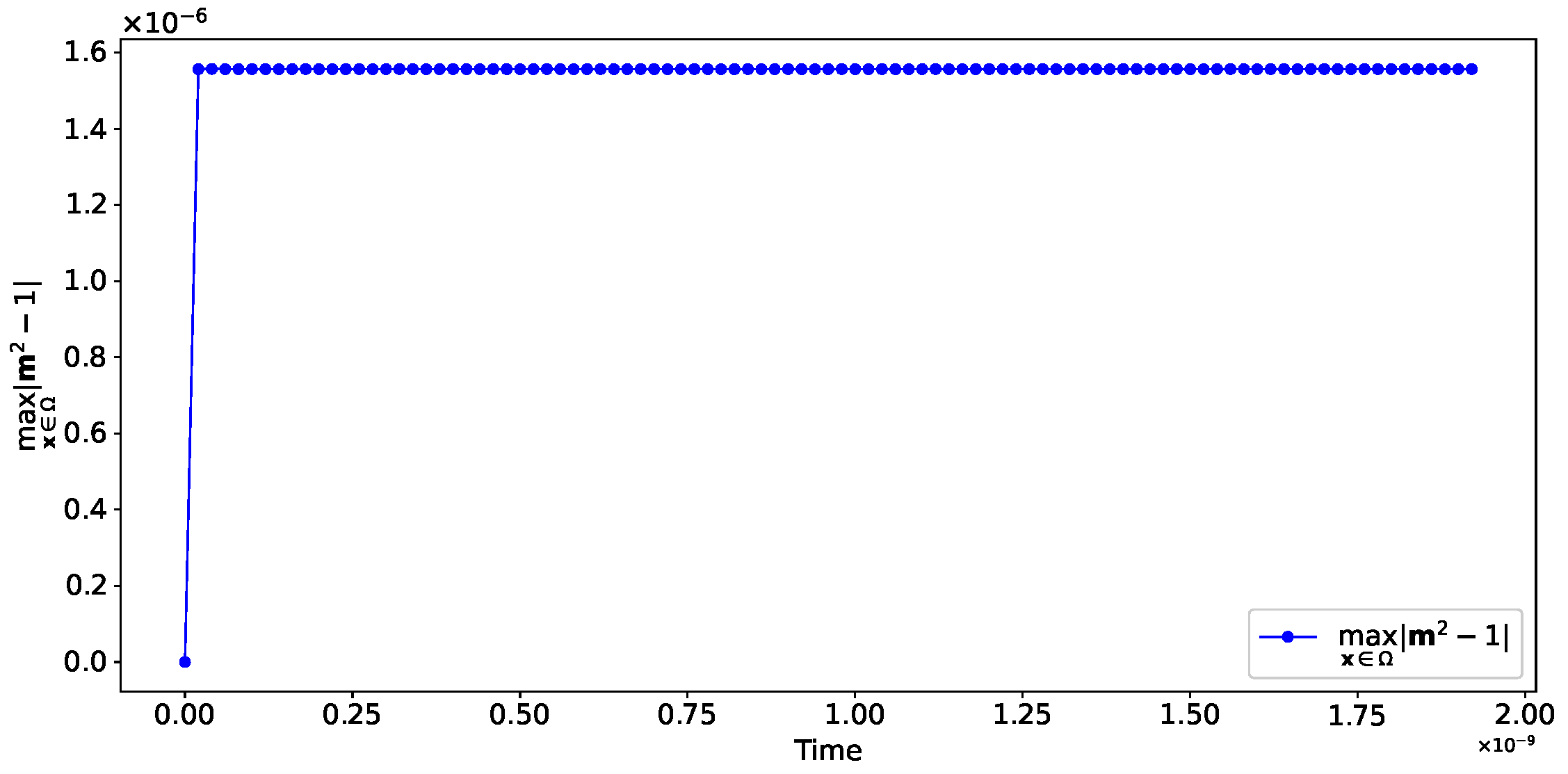
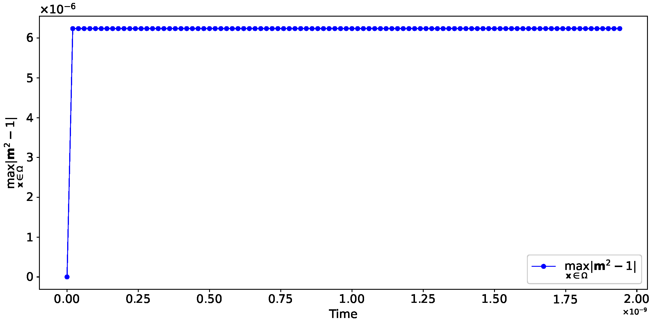
3. Preservation of Magnetization Magnitude

In this section, we analyze the preservation of the magnetization magnitude $|{\mathit{m}}^n|$ of the discrete scheme Equation (13).

Multiplying both sides of Equation (13) by $({\mathit{m}}^{n+1}+{\mathit{m}}^n)$, it can be obtained that

$$\frac{{\left|{\mathit{m}}^{n+1}\right|}^2-{\left|{\mathit{m}}^n\right|}^2}{\Delta t}=S_{\mathit{m}\times \mathit{D}}·\left({\mathit{m}}^{n+1}+{\mathit{m}}^n\right).$$

(23)

To analyze the preservation of magnetization magnitude, the items on the right-hand side of Equation (23) should be discussed. To this end, a series of lemmas are provided.

Lemma 2. 

According to $B_j$ in Equation (10), we have

$$\begin{array}{ccc}\hfill S_{\mathit{m}\times \mathit{D}}·\left({\mathit{m}}^{n+1}+{\mathit{m}}^n\right)& =& 2\sum _{j=0}^p\Delta t^{2j}\left(\sum _{i=0}^j\frac{B_{2i}}{\left(2i\right)!(2j-2i)!2^{2j-2i}}{\overline{\mathit{m}}}^{(2i+1)}·{\overline{\mathit{m}}}^{(2j-2i)}\right)+\mathcal{O}(\Delta t^{2p+2}).\hfill \end{array}$$

(24)

Proof. 

Firstly, by Equation (15) with $c=\pm 1/2$, we have

$${\mathit{m}}^{n+1}+{\mathit{m}}^n=\sum _{j=0}^{\infty }\frac{\Delta t^j}{j!}\left(\frac{1}{2^j}+\frac{{(-1)}^j}{2^j}\right){\overline{\mathit{m}}}^{\left(j\right)}=2\sum _{j=0}^{\infty }\frac{\Delta t^{2j}}{\left(2j\right)!2^{2j}}{\overline{\mathit{m}}}^{\left(2j\right)}.$$

(25)

Then, combining Equations (21) and (25), it is obtained that

$$\begin{array}{ccc}\hfill S_{\mathit{m}\times \mathit{D}}·\left({\mathit{m}}^{n+1}+{\mathit{m}}^n\right)& =& \left(\sum _{s=0}^{\infty }{B}_{2s}\frac{\Delta t^{2s}}{\left(2s\right)!}{\overline{\mathit{m}}}^{(2s+1)}\right)·\left(2\sum _{j=0}^{\infty }\frac{\Delta t^{2j}}{\left(2j\right)!2^{2j}}{\overline{\mathit{m}}}^{\left(2j\right)}\right)\hfill \\ \hfill & =& \sum _{j=0}^{\infty }\sum _{s=0}^j{B}_{2s}\left(\frac{2\Delta t^{2s}\Delta t^{2j-2s}}{\left(2s\right)!(2j-2s)!2^{2j-2s}}{\overline{\mathit{m}}}^{(2s+1)}·{\overline{\mathit{m}}}^{(2j-2s)}\right)\hfill \\ \hfill & =& 2\sum _{j=0}^{\infty }\Delta t^{2j}\left(\sum _{s=0}^j\frac{B_{2s}}{\left(2s\right)!(2j-2s)!2^{2j-2s}}{\overline{\mathit{m}}}^{(2s+1)}·{\overline{\mathit{m}}}^{(2j-2s)}\right),\hfill \end{array}$$

(26)

which completes the proof with Equation (23). □

Lemma 3. 

For any positive integer k, there exists

$$\sum _{i=1}^{2k-1}{C}_{2k}^i{\overline{\mathit{m}}}^{(2k-i)}·\left(\sum _{s=0}^{i-1}{C}_i^s({\overline{\mathit{m}}}^{(i-s)}\times {\overline{\mathit{D}}}^{\left(s\right)})\right)=0.$$

(27)

Proof. 

By rearrangement and taking $l=i-s$, we have

$$\begin{array}{l}{\displaystyle \sum _{i=1}^{2k-1}{C}_{2k}^i{\overline{\mathit{m}}}^{(2k-i)}·\left(\sum _{s=0}^{i-1}{C}_i^s({\overline{\mathit{m}}}^{(i-s)}\times {\overline{\mathit{D}}}^{\left(s\right)})\right)}\\ \hspace{1em}={\displaystyle \sum _{s=0}^{2k-2}}{\displaystyle \sum _{i=s+1}^{2k-1}}{C}_{2k}^i{C}_i^s{\overline{\mathit{m}}}^{(2k-i)}·({\overline{\mathit{m}}}^{(i-s)}\times {\overline{\mathit{D}}}^{\left(s\right)})\\ \hspace{1em}={\displaystyle \sum _{s=0}^{2k-2}}{\displaystyle \sum _{l=1}^{2k-1-s}}{C}_{2k}^{l+s}{C}_{l+s}^s{\overline{\mathit{m}}}^{(2k-l-s)}·({\overline{\mathit{m}}}^{\left(l\right)}\times {\overline{\mathit{D}}}^{\left(s\right)}).\end{array}$$

(28)

We introduce the notation

$$T_1:=\sum _{s=0}^{2k-2}\sum _{l=1}^{2k-1-s}{C}_{2k}^{l+s}{C}_{l+s}^s{\overline{\mathit{m}}}^{(2k-l-s)}·({\overline{\mathit{m}}}^{\left(l\right)}\times {\overline{\mathit{D}}}^{\left(s\right)}).$$

(29)

Taking $h=2k-s-l$, and noticing that

$$C_{2k}^{2k-h}{C}_{2k-h}^s=\frac{\left(2k\right)!(2k-h)!}{h!(2k-h)!(2k-h-s)!s!}=\frac{\left(2k\right)!(h+s)!}{h!(h+s)!(2k-h-s)!s!}=C_{2k}^{h+s}{C}_{h+s}^s,$$

(30)

$T_1$ can be transformed into the following form:

$$\begin{array}{ccc}\hfill T_1& =& \sum _{s=0}^{2k-2}\sum _{h=1}^{2k-1-s}{C}_{2k}^{2k-h}{C}_{2k-h}^s{\overline{\mathit{m}}}^{\left(h\right)}·({\overline{\mathit{m}}}^{(2k-h-s)}\times {\overline{\mathit{D}}}^{\left(s\right)})\hfill \\ \hfill & =& \sum _{s=0}^{2k-2}\sum _{h=1}^{2k-1-s}{C}_{2k}^{h+s}{C}_{h+s}^s{\overline{\mathit{m}}}^{\left(h\right)}·({\overline{\mathit{m}}}^{(2k-h-s)}\times {\overline{\mathit{D}}}^{\left(s\right)})\hfill \\ \hfill & =& -\sum _{s=0}^{2k-2}\sum _{h=1}^{2k-1-s}{C}_{2k}^{h+s}{C}_{h+s}^s{\overline{\mathit{m}}}^{(2k-h-s)}·({\overline{\mathit{m}}}^{\left(h\right)}\times {\overline{\mathit{D}}}^{\left(s\right)})\hfill \\ \hfill & =& -T_1.\hfill \end{array}$$

(31)

The conclusion is obtained accordingly. □

Lemma 4. 

According to Equation (11), we have

$$\sum _{i=0}^k\frac{B_{2i}}{\left(2i\right)!(2k-2i)!2^{2k-2i}}{\overline{\mathit{m}}}^{(2i+1)}·{\overline{\mathit{m}}}^{(2k-2i)}=0,\mathit{for}k=0,1,2,\cdots ,p.$$

(32)

Proof. 

Firstly, the left-hand side of Equation (32) is split as

$$\sum _{i=0}^k\frac{B_{2i}}{\left(2i\right)!(2k-2i)!2^{2k-2i}}{\overline{\mathit{m}}}^{(2i+1)}·{\overline{\mathit{m}}}^{(2k-2i)}:=I_1+I_2,$$

(33)

where

$$\begin{array}{ccc}& I_1& {\displaystyle =\sum _{i=0}^{k-1}\frac{B_{2i}}{\left(2i\right)!(2k-2i)!2^{2k-2i}}{\overline{\mathit{m}}}^{(2i+1)}·{\overline{\mathit{m}}}^{(2k-2i)},}\hfill \\ & I_2& {\displaystyle =\frac{B_{2k}}{\left(2k\right)!}{\overline{\mathit{m}}}^{(2k+1)}·\overline{\mathit{m}}.}\hfill \end{array}$$

By using Equation (18) with $s=2k$, $I_2$ can be written as

$$\begin{array}{ccc}\hfill I_2& =& \frac{B_{2k}}{\left(2k\right)!}{\overline{\mathit{m}}}^{(2k+1)}·\overline{\mathit{m}}\hfill \\ \hfill & =& \frac{B_{2k}}{\left(2k\right)!}\left(-\sum _{i=0}^{2k}{C}_{2k}^i{\overline{\mathit{m}}}^{(2k-i)}\times {\overline{\mathit{D}}}^{\left(i\right)}\right)·\overline{\mathit{m}}\hfill \\ \hfill & =& -\frac{B_{2k}}{\left(2k\right)!}\left(\sum _{i=0}^{2k}{C}_{2k}^i{\overline{\mathit{m}}}^{(2k-i)}·\left({\overline{\mathit{D}}}^{\left(i\right)}\times \overline{\mathit{m}}\right)\right).\hfill \end{array}$$

Next, using the above equation, by splitting and using Equations (17) and (19), $I_2$ can be written as

$$\begin{array}{ccc}\hfill I_2& =& -\frac{B_k}{\left(2k\right)!}{C}_{2k}^{2k}\overline{\mathit{m}}·\left({\overline{\mathit{D}}}^{\left(2k\right)}\times \overline{\mathit{m}}\right)-\frac{B_{2k}}{\left(2k\right)!}\sum _{i=1}^{2k-1}{C}_{2k}^i{\overline{\mathit{m}}}^{(2k-i)}·\left({\overline{\mathit{D}}}^{\left(i\right)}\times \overline{\mathit{m}}\right)\hfill \\ \hfill & & -\frac{B_{2k}}{\left(2k\right)!}{C}_{2k}^0{\overline{\mathit{m}}}^{\left(2k\right)}·(\overline{\mathit{D}}\times \overline{\mathit{m}})\hfill \\ \hfill & =& -\frac{B_{2k}}{\left(2k\right)!}\sum _{i=1}^{2k-1}{C}_{2k}^i{\overline{\mathit{m}}}^{(2k-i)}·\left({\overline{\mathit{D}}}^{\left(i\right)}\times \overline{\mathit{m}}\right)-\frac{B_{2k}}{\left(2k\right)!}{\overline{\mathit{m}}}^{\left(2k\right)}·{\overline{\mathit{m}}}_t\hfill \\ \hfill & =& -\frac{B_{2k}}{\left(2k\right)!}\sum _{i=1}^{2k-1}{C}_{2k}^i{\overline{\mathit{m}}}^{(2k-i)}·\left({\overline{\mathit{m}}}^{(i+1)}+\sum _{s=0}^{i-1}{C}_i^s\left({\overline{\mathit{m}}}^{(i-s)}\times {\overline{\mathit{D}}}^{\left(s\right)}\right)\right)-\frac{B_{2k}}{\left(2k\right)!}{\overline{\mathit{m}}}^{\left(2k\right)}·{\overline{\mathit{m}}}_t\hfill \\ \hfill & =& -\frac{B_{2k}}{\left(2k\right)!}\sum _{i=0}^{2k-1}{C}_{2k}^i{\overline{\mathit{m}}}^{(2k-i)}·{\overline{\mathit{m}}}^{(i+1)}-\frac{B_{2k}}{\left(2k\right)!}\sum _{i=1}^{2k-1}{C}_{2k}^i{\overline{\mathit{m}}}^{(2k-i)}·\sum _{s=0}^{i-1}{C}_i^s\left({\overline{\mathit{m}}}^{(i-s)}\times {\overline{\mathit{D}}}^{\left(s\right)}\right)\hfill \\ \hfill & :=& I_{21}+I_{22}.\hfill \end{array}$$

(34)

By splitting $I_{21}$ into odd terms and even terms, we have

$$\begin{array}{ccc}\hfill I_{21}& =& -\frac{B_{2k}}{\left(2k\right)!}\sum _{i=0}^{k-1}{C}_{2k}^{2i}{\overline{\mathit{m}}}^{(2k-2i)}·{\overline{\mathit{m}}}^{(2i+1)}-\frac{B_{2k}}{\left(2k\right)!}\sum _{i=0}^{k-1}{C}_{2k}^{2i+1}{\overline{\mathit{m}}}^{(2i+1)}·{\overline{\mathit{m}}}^{(2k-2i)}\hfill \\ \hfill & =& -B_{2k}\sum _{i=0}^{k-1}\left(\frac{1}{\left(2i\right)!(2k-2i)!}+\frac{1}{(2i+1)!(2k-2i-1)!}\right){\overline{\mathit{m}}}^{(2i+1)}·{\overline{\mathit{m}}}^{(2k-2i)}.\hfill \end{array}$$

(35)

Noticing that Lemma 3 indicates $I_{22}=0$, then using Equations (33)–(35) and (11), we have

$$\begin{array}{l}{\displaystyle \sum _{i=0}^k\frac{B_{2i}}{\left(2i\right)!(2k-2i)!2^{2k-2i}}{\overline{\mathit{m}}}^{(2i+1)}·{\overline{\mathit{m}}}^{(2k-2i)}}\\ \hspace{1em}={\displaystyle \sum _{i=0}^{k-1}}\left(\frac{B_{2i}}{\left(2i\right)!(2k-2i)!2^{(2k-2i)}}-\frac{B_{2k}}{\left(2i\right)!(2k-2i)!}-\frac{B_{2k}}{(2i+1)!(2k-2i-1)!}\right){\overline{\mathit{m}}}^{(2i+1)}·{\overline{\mathit{m}}}^{(2k-2i)}\\ \hspace{1em}={\displaystyle \sum _{i=0}^{k-1}}\frac{\left((2k+1)-(2i+1)-(2k-2i)\right)}{(2k+1)(2i+1)!(2k-2i)!2^{2k}}{\overline{\mathit{m}}}^{(2i+1)}·{\overline{\mathit{m}}}^{(2k-2i)}\\ \hspace{1em}=0,\end{array}$$

(36)

which completes the proof. □

By using the aforementioned lemmas, we analyze the preservation of magnetization magnitude of the discrete scheme Equation (13) in the following theorem.

Theorem 1. 

For the discrete scheme Equation (13) based on $(p+1)$ Gauss–Legendre quadrature nodes and weights, we have

$$|{\mathit{m}}^{n+1}{|}^2-{\left|{\mathit{m}}^n\right|}^2\sim \mathcal{O}(\Delta t^{2p+3}).$$

(37)

Proof. 

Using Lemma 2, we have

$$\begin{array}{ccc}\hfill |{\mathit{m}}^{n+1}{|}^2-{\left|{\mathit{m}}^n\right|}^2& =& 2\sum _{j=0}^p\Delta t^{2j+1}\left(\sum _{i=0}^j\frac{B_{2i}}{\left(2i\right)!(2j-2i)!2^{(2j-2s)}}{\overline{\mathit{m}}}^{(2i+1)}·{\overline{\mathit{m}}}^{(2j-2i)}\right)+O(\Delta t^{2p+3}).\hfill \end{array}$$

Further, by applying Lemma 4 to the above equation, the conclusion can be obtained. □

Remark 2. 

Theorem 1 is still valid for the case where the effective field includes the external field, since the specific expression of D has not been utilized in Section 3.

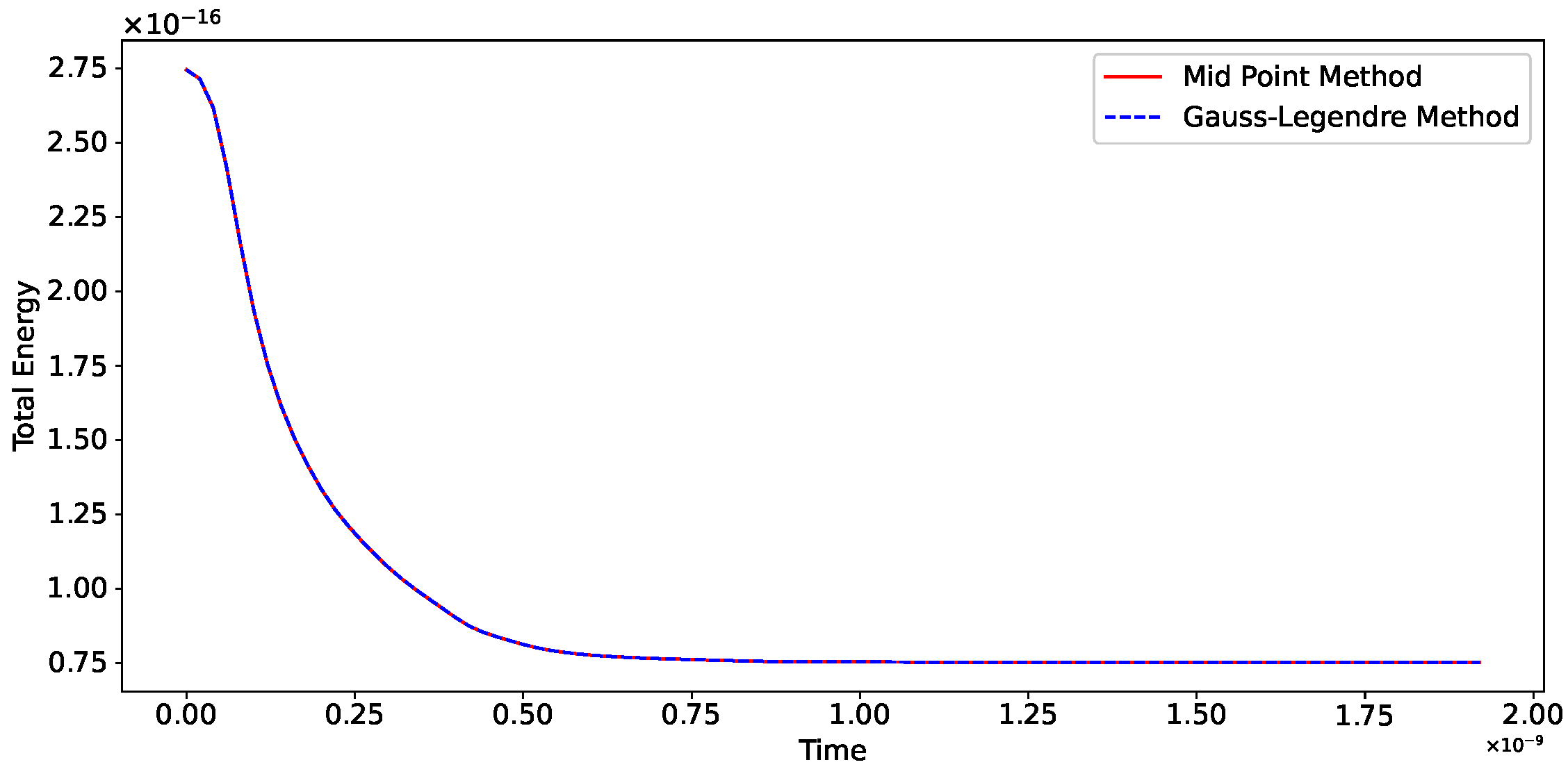
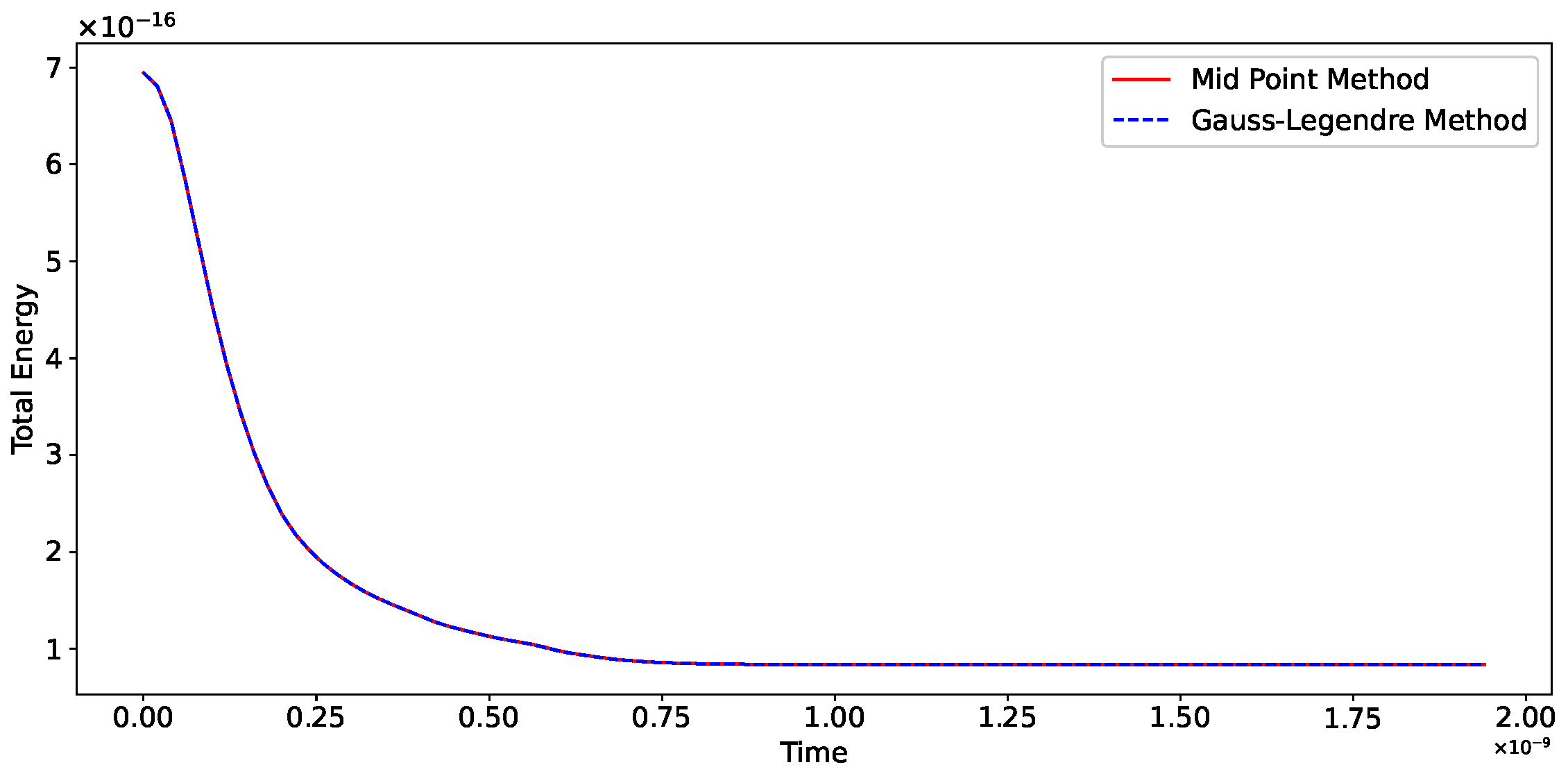
4. Preservation of the Lyapunov Structure

In micromagnetics, the Lyapunov structure implies the free energy $g\left(\mathit{m}\right)$ in Equation (5) is a decreasing function of time, which can be expressed as

$$\frac{\mathrm{d}g\left(\mathit{m}\right(t\left)\right)}{\mathrm{d}t}=-\alpha {\int }_{\Omega }|\frac{\partial \mathit{m}\left(t\right)}{\partial t}{|}^2\mathrm{d}\mathit{x}.$$

(38)

In this section, we analyze the preservation of Lyapunov structure within the discrete scheme Equation (13).

The magnetic body $\Omega$ is assumed to be subdivided by spatial discretization techniques, such as finite difference methods, finite element methods, etc., with a total of N degrees of freedom.

After spatial discretization, the discrete scheme Equation (13) can be rewritten as

$$\begin{array}{c}\hfill \frac{{\underline{\mathit{m}}}^{n+1}-{\underline{\mathit{m}}}^n}{\Delta t}=-\sum _{i=0}^p{\omega }_i\underline{\mathit{m}}({\overline{t}}_n+a_i\Delta t)\odot \underline{\mathit{D}}({\overline{t}}_n+a_i\Delta t),\end{array}$$

(39)

where

$$\begin{array}{c}\hfill \underline{\mathit{m}}={(m_{1,1},\cdots ,m_{1,N},m_{2,1},\cdots ,m_{2,N},m_{3,1},\cdots ,m_{3,N})}^T\in {\mathbb{R}}^{3N}.\end{array}$$

(40)

${\mathit{m}}_{i,j}$ denotes the ith component of the magnetization vector field $\mathit{m}\in {\mathbb{R}}^3$ at the jth degree of freedom and the operator ⊙ is defined as for any $\underline{\mathit{a}},\underline{\mathit{b}}\in {\mathbb{R}}^{3N}$,

$$\begin{array}{c}\hfill \underline{\mathit{c}}=\underline{\mathit{a}}\odot \underline{\mathit{b}}\in {\mathbb{R}}^{3N}\end{array}$$

(41)

with $(c_{1,j},c_{2,j},c_{3,j})=(a_{1,j},a_{2,j},a_{3,j})\times (b_{1,j},b_{2,j},b_{3,j}),j=1,2,\cdots ,N$.

For the fully discrete scheme Equation (39), the free energy $g\left(\mathit{m}\right)$ and $\underline{\mathit{D}}=\underline{{\mathit{h}}_{\mathrm{eff}}}-\alpha {\underline{\mathit{m}}}_t$ can be written as (see Equations (25) and (26) of reference [21]):

$$\begin{array}{c}\hfill g\left(\underline{\mathit{m}}\right)=\frac{1}{2}\underline{\mathit{m}}·C·\underline{\mathit{m}},\end{array}$$

(42)

$$\begin{array}{c}\hfill \underline{\mathit{D}}=-C·\underline{\mathit{m}}-\alpha {\underline{\mathit{m}}}_t,\end{array}$$

(43)

where C is a $3N\times 3N$ symmetric matrix.

Next, we analyze the preservation of the Lyapunov structure in the discrete scheme Equation (39).

Theorem 2. 

For the discrete scheme Equation (39), we have

$$\frac{g\left({\underline{\mathit{m}}}^{n+1}\right)-g\left({\underline{\mathit{m}}}^n\right)}{\Delta t}=-\alpha {\left|\frac{{\underline{\mathit{m}}}^{n+k}-{\underline{\mathit{m}}}^{n+k-1}}{\Delta t}\right|}^2+\mathcal{O}(\Delta t^2).$$

(44)

Proof. 

Firstly, we introduce the notation

$$T:=-C·\frac{{\underline{\mathit{m}}}^{n+1}+{\underline{\mathit{m}}}^n}{2}-\alpha \frac{{\underline{\mathit{m}}}^{n+1}-{\underline{\mathit{m}}}^n}{\Delta t}.$$

(45)

Additionally, using Equations (25) and (22), T can be expanded as

$$\begin{array}{ccc}\hfill T& =& \left(-C·\left(\sum _{j=0}^{\infty }\frac{\Delta t^{2j}}{\left(2j\right)!2^{2j}}{\overline{\mathit{m}}}^{\left(2j\right)}\right)-\alpha \left(\sum _{j=0}^{\infty }\frac{\Delta t^{2j}}{2^{2j}(2j+1)!}·{\overline{\mathit{m}}}^{(2j+1)}\right)\right)\hfill \\ \hfill & =& -C·\overline{\underline{\mathit{m}}}-\alpha {\overline{\underline{\mathit{m}}}}_t+\mathcal{O}(\Delta t^2).\hfill \end{array}$$

(46)

Multiplying both sides of Equation (39) by T defined in Equation (45), using the symmetry of C and Equation (42), we have

$$\begin{array}{l}{\displaystyle -\frac{g\left({\underline{\mathit{m}}}^{n+1}\right)-g\left({\underline{\mathit{m}}}^{n-1}\right)}{\Delta t}-\alpha {\left|\frac{{\underline{\mathit{m}}}^{n+1}-{\underline{\mathit{m}}}^n}{\Delta t}\right|}^2}\\ \hspace{1em}=\left(-{\displaystyle \sum _{i=0}^p}{\omega }_i\underline{\mathit{m}}({\overline{t}}_n+a_i\Delta t)\odot \underline{\mathit{D}}({\overline{t}}_n+a_i\Delta t)\right)·T.\end{array}$$

(47)

By using the similar technique as in Equation (21) with Equation (11) and Equation (46), the right-hand side of Equation (47) can be written as

$$\begin{array}{c}\hfill \left({\overline{\underline{\mathit{m}}}}_t+\mathcal{O}(\Delta t^2)\right)·\left(-C·\overline{\underline{\mathit{m}}}-\alpha {\overline{\underline{\mathit{m}}}}_t+\mathcal{O}(\Delta t^2)\right).\end{array}$$

(48)

Substituting (48) into Equation (47), and using Equations (43) and (17), we have

$$-\frac{g\left({\underline{\mathit{m}}}^{n+1}\right)-g\left({\underline{\mathit{m}}}^{n-1}\right)}{\Delta t}-\alpha {\left|\frac{{\underline{\mathit{m}}}^{n+1}-{\underline{\mathit{m}}}^n}{\Delta t}\right|}^2=\mathcal{O}(\Delta t^2),$$

(49)

which completes the proof. □

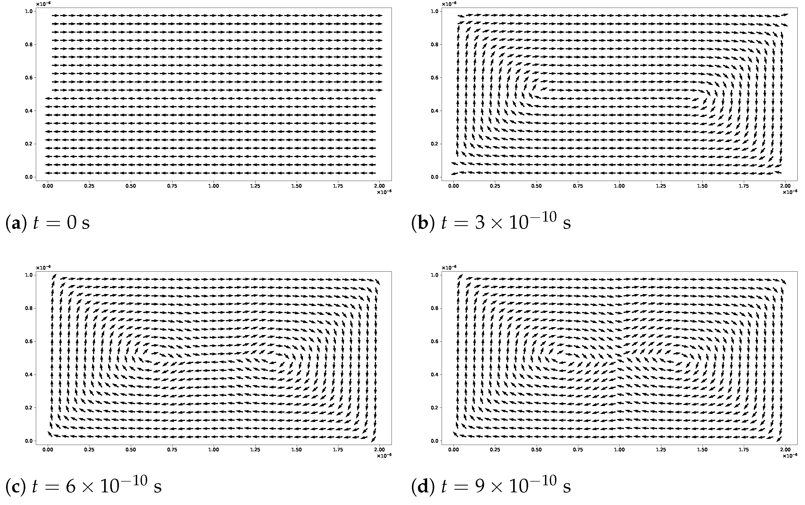
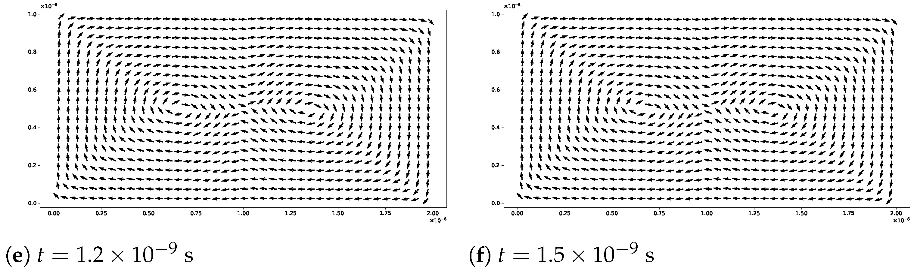
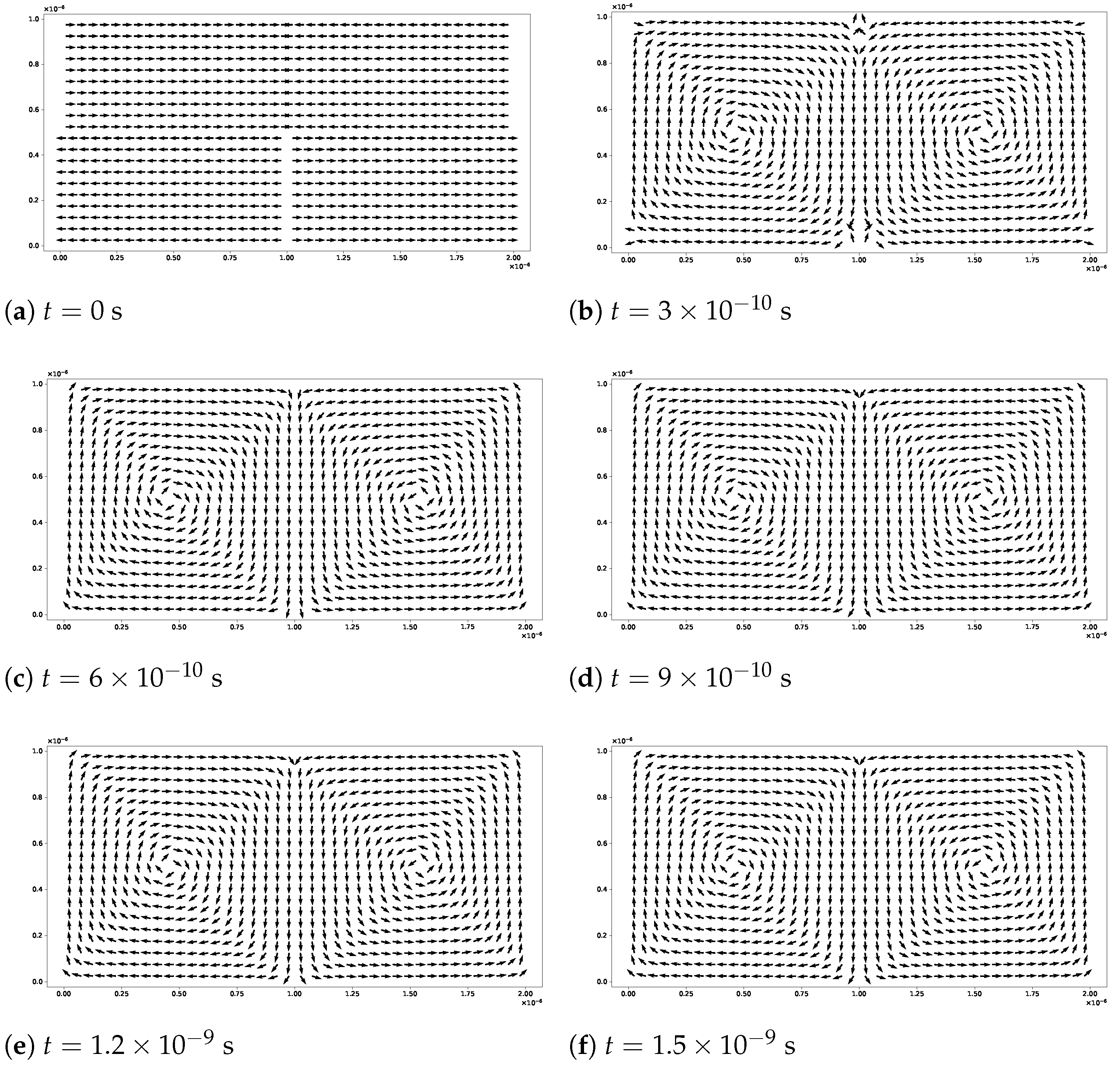
5. Numerical Experiments

In this section, some numerical experiments are presented to verify the effectiveness of the discrete scheme Equation (13).

5.1. Accuracy Test

In this subsection, the accuracy of the discrete scheme Equation (13) with a predetermined exact solution is tested as follows.

Example 1. 

The problem is presented as

$$\frac{\partial \mathit{m}}{\partial t}=-\mathit{m}\times \left(\Delta \mathit{m}-\alpha \frac{\partial \mathit{m}}{\partial t}\right)+\mathit{f}\mathit{in}\Omega \times T,$$

(50)

with $\alpha =0.1$, the space domain $\Omega =[0,1]\times [0,1]\times [0,1]$, and the time domain $T=[\pi /4,\pi /4+0.2]$. The exact solution is given as

$${\mathit{m}}_e=\left(\begin{array}{c}sin(1/t)cos\left(x^2{y}^2{z}^2{(1-x)}^2{(1-y)}^2{(1-z)}^2\right)\\ sin(1/t)sin\left(x^2{y}^2{z}^2{(1-x)}^2{(1-y)}^2{(1-z)}^2\right)\\ cos(1/t)\end{array}\right),$$

(51)

and $\mathit{f}$ is chosen according to Equation (50) and the exact solution Equation (51).

In this experiment, the temporal discrete scheme Equation (14), as one special case of the general scheme Equation (13) with $p=1$, of fourth order in time and second order in space, is implemented:

$$\begin{array}{l}{\displaystyle \frac{{\mathit{m}}^{n+1}-{\mathit{m}}^n}{\Delta t}}\\ \hspace{1em}={\displaystyle \frac{1}{2}}\left(-{\mathit{m}}_h\left({\overline{t}}_n-\frac{\Delta t}{2\sqrt{3}}\right)\times {\Delta }_h{\mathit{m}}_h\left({\overline{t}}_n-\frac{\Delta t}{2\sqrt{3}}\right)+\alpha {\mathit{m}}_h\left({\overline{t}}_n-\frac{\Delta t}{2\sqrt{3}}\right)\times {\mathit{m}}_{t,h}\left({\overline{t}}_n-\frac{\Delta t}{2\sqrt{3}}\right)\right)\\ \hspace{1em}\hspace{1em}+{\displaystyle \frac{1}{2}}\left(-{\mathit{m}}_h\left({\overline{t}}_n+\frac{\Delta t}{2\sqrt{3}}\right)\times {\Delta }_h{\mathit{m}}_h\left({\overline{t}}_n+\frac{\Delta t}{2\sqrt{3}}\right)+\alpha {\mathit{m}}_h\left({\overline{t}}_n+\frac{\Delta t}{2\sqrt{3}}\right)\times {\mathit{m}}_{t,h}\left({\overline{t}}_n+\frac{\Delta t}{2\sqrt{3}}\right)\right)\\ \hspace{1em}\hspace{1em}+{\displaystyle \frac{1}{2}}\mathit{f}\left({\overline{t}}_n-\frac{\Delta t}{2\sqrt{3}}\right)+{\displaystyle \frac{1}{2}}\mathit{f}\left({\overline{t}}_n+\frac{\Delta t}{2\sqrt{3}}\right),\end{array}$$

(52)

where

$$\begin{array}{ccc}\hfill {\mathit{m}}_h\left({\overline{t}}_n-\frac{\Delta t}{2\sqrt{3}}\right)& =& {\tilde{\alpha }}_{-2}{\mathit{m}}^{n-2}+{\tilde{\alpha }}_{-1}{\mathit{m}}^{n-1}+{\tilde{\alpha }}_0{\mathit{m}}^n+{\tilde{\alpha }}_1{\mathit{m}}^{n+1},\hfill \\ \hfill {\mathit{m}}_{t,h}\left({\overline{t}}_n-\frac{\Delta t}{2\sqrt{3}}\right)& =& \left({\tilde{\beta }}_{-2}{\mathit{m}}^{n-2}+{\tilde{\beta }}_{-1}{\mathit{m}}^{n-1}+{\tilde{\beta }}_0{\mathit{m}}^n+{\tilde{\beta }}_1{\mathit{m}}^{n+1}\right)/\Delta t,\hfill \\ \hfill {\mathit{m}}_h\left({\overline{t}}_n+\frac{\Delta t}{2\sqrt{3}}\right)& =& {\overline{\alpha }}_{-2}{\mathit{m}}^{n-2}+{\overline{\alpha }}_{-1}{\mathit{m}}^{n-1}+{\overline{\alpha }}_0{\mathit{m}}^n+{\overline{\alpha }}_1{\mathit{m}}^{n+1},\hfill \\ \hfill {\mathit{m}}_{t,h}\left({\overline{t}}_n+\frac{\Delta t}{2\sqrt{3}}\right)& =& \left({\overline{\beta }}_{-2}{\mathit{m}}^{n-2}+{\overline{\beta }}_{-1}{\mathit{m}}^{n-1}+{\overline{\beta }}_0{\mathit{m}}^n+{\overline{\beta }}_1{\mathit{m}}^{n+1}\right)/\Delta t,\hfill \end{array}$$

the coefficients $\left\{\tilde{\alpha }\right\}$, $\left\{\tilde{\beta }\right\}$, $\left\{\overline{\alpha }\right\}$, $\left\{\overline{\beta }\right\}$, are chosen to achieve fourth-order approximations for the following four terms:

$$\mathit{m}\left({\overline{t}}_n-\frac{\Delta t}{2\sqrt{3}}\right),{\mathit{m}}_t\left({\overline{t}}_n-\frac{\Delta t}{2\sqrt{3}}\right),\mathit{m}\left({\overline{t}}_n+\frac{\Delta t}{2\sqrt{3}}\right),{\mathit{m}}_t\left({\overline{t}}_n+\frac{\Delta t}{2\sqrt{3}}\right),$$

respectively, and ${\Delta }_h$ is a discrete Laplace operator of second-order central difference.

In this case, the initial value ${\mathit{m}}^0$ is provided by the exact solution, and ${\mathit{m}}^1$ and ${\mathit{m}}^2$ are obtained by using the fourth-order Runge–Kutta method. Noticing that the fully discrete scheme (52) is implicit, an explicit iteration method is applied to solve this discrete scheme with initial value ${\mathit{m}}^2$ and tolerance error $tol={10}^{-8}$. In this numerical test, the spatial mesh size h and temporal step size $\Delta t$ are selected at a fixed ratio of $\Delta t^2/h$. In

Table 1. Convergence test for Example 1.

$\mathbf{\Delta }\mathit{t}$	h	$\parallel {\mathit{m}}_{\mathit{h}}-{\mathit{m}}_{\mathit{e}}{\parallel }_{\mathit{\infty }}$	Order
2 × 10−4	2 × 10−1	2.6011 × 10−5	-
1.41 × 10−4	1 × 10−1	6.6369 × 10−6	3.9411
1 × 10−4	5 × 10−2	1.6495 × 10−6	4.0170
7.07 × 10−5	2.5 × 10−2	4.1832 × 10−7	3.9586

, the difference between the numerical solution ${\mathit{m}}_h$ and the exact solution ${\mathit{m}}_e$ at time $t=\pi /4+0.2$ is described as the maximum errors ${∥{\mathit{m}}_h-{\mathit{m}}_e∥}_{\infty }$ for different temporal step size $\Delta t$. From Table 1, it can be observed that the numerical order is around 4, which basically fits the theoretical conclusion of fourth order in Lemma 1 with $p=1$.

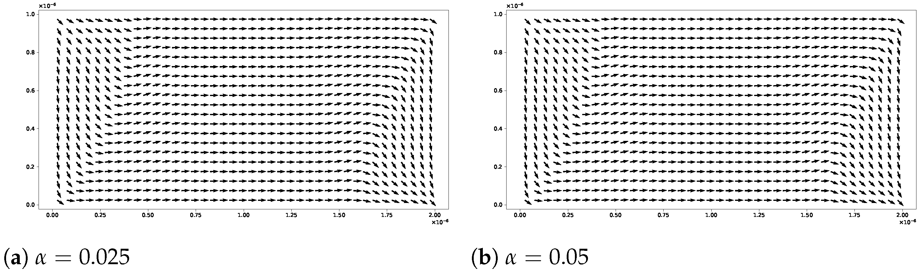
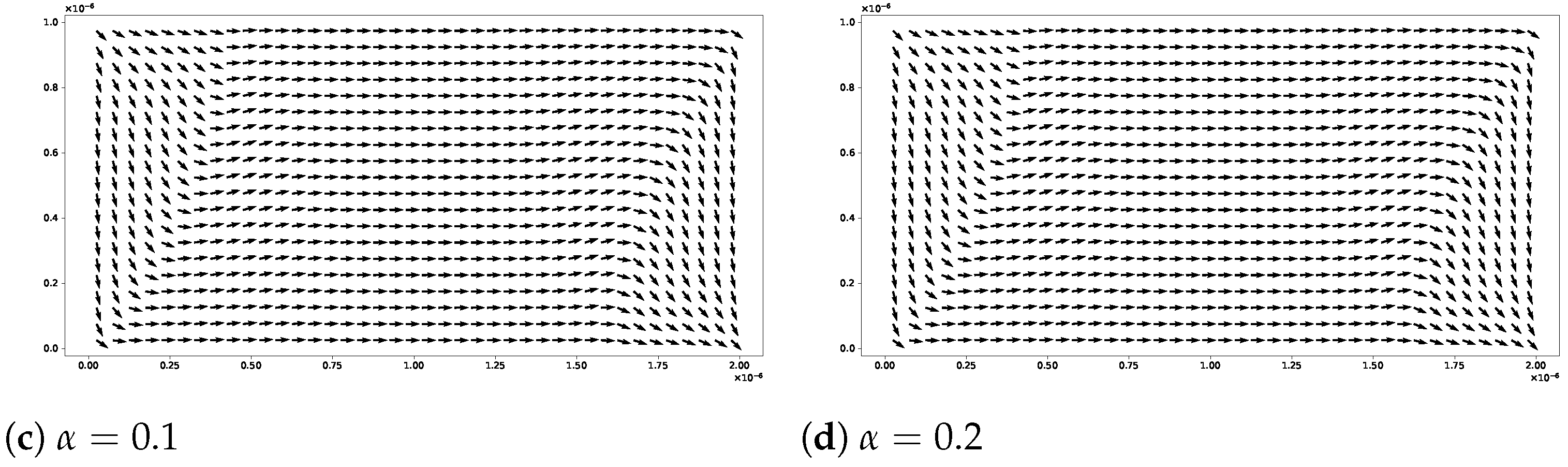
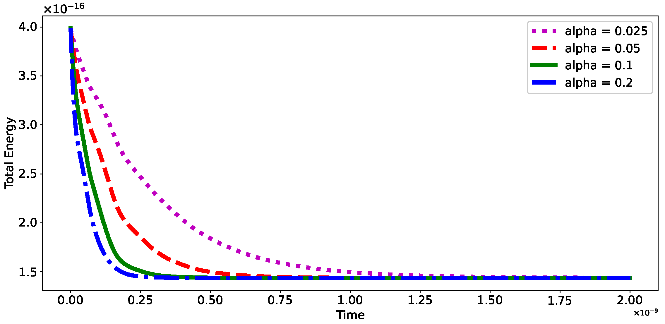
5.2. Numerical Simulations

In this subsection, a series of numerical simulations is conducted to validate the effectiveness and applicability of the proposed numerical scheme (13).

In the absence of specific indications or declarations, it is assumed that the equilibrium state of the magnetization has been reached when

$$\underset{l=1,\cdots ,N}{max}|{\mathit{m}}_l\times {\mathit{h}}_{\mathrm{eff},l}|\le {10}^{-5}.$$

(53)

Example 2. 

Let Ω be a $2 \mu m\times 1 \mu m\times 0.02 \mu m$-sized ferromagnetic thin film. We investigate the LLG equation (2) with $\alpha =0.1$ and $\gamma =2.211\times {10}^5 m/\left(\mathit{As}\right)$. The effective field is expressed as

$$\begin{array}{c}\hfill {\mathit{h}}_{\mathrm{eff}}=\frac{2C_{ex}}{{\mu }_0{M}_s^2}\Delta \mathit{m}+\frac{2K_u}{{\mu }_0{M}_s^2}{\mathit{e}}_{an}\left(\mathit{m}·{\mathit{e}}_{an}\right)+{\mathit{h}}_s,\end{array}$$

(54)

where $C_{ex}=1.3\times {10}^{-11} J/m$, ${\mu }_0=4\pi \times {10}^{-7} N/A^2$, $M_s=8.0\times {10}^5 A/m$, $K_u=5.0\times {10}^2 J/m^3$, ${\mathit{e}}_{an}=(1,0,0)$, and the stray field ${\mathit{h}}_s$ is given as

$${\mathit{h}}_s=-{\nabla }_{\mathit{x}}\left({\int }_{\Omega }{\nabla }_{\mathit{y}}\left(\frac{1}{4\pi |\mathit{x}-\mathit{y}|}\right)·\mathit{m}\left(\mathit{y}\right)\mathrm{d}\mathit{y}\right).$$

(55)

The two-point Gauss–Legendre fully discrete scheme is employed as follows:

$$\begin{array}{l}{\displaystyle \frac{{\mathit{m}}^{n+1}-{\mathit{m}}^n}{\Delta t}}\\ \hspace{1em}={\displaystyle \frac{1}{2}}\left(-{\mathit{m}}_h\left({\overline{t}}_n-\frac{\Delta t}{2\sqrt{3}}\right)\times {\mathit{h}}_{\mathrm{eff}}\left({\overline{t}}_n-\frac{\Delta t}{2\sqrt{3}}\right)+\alpha {\mathit{m}}_h\left({\overline{t}}_n-\frac{\Delta t}{2\sqrt{3}}\right)\times {\mathit{m}}_{t,h}\left({\overline{t}}_n-\frac{\Delta t}{2\sqrt{3}}\right)\right)\\ \hspace{1em}+{\displaystyle \frac{1}{2}}\left(-{\mathit{m}}_h\left({\overline{t}}_n+\frac{\Delta t}{2\sqrt{3}}\right)\times {\mathit{h}}_{\mathrm{eff}}\left({\overline{t}}_n+\frac{\Delta t}{2\sqrt{3}}\right)+\alpha {\mathit{m}}_h\left({\overline{t}}_n+\frac{\Delta t}{2\sqrt{3}}\right)\times {\mathit{m}}_{t,h}\left({\overline{t}}_n+\frac{\Delta t}{2\sqrt{3}}\right)\right),\end{array}$$

(56)

with the same notations as in Example 1.

To evaluate the effectiveness of the numerical scheme (56), we employ a fully discrete mid-point method as a reference, and its formula is expressed as

$$\begin{array}{c}\hfill \frac{{\mathit{m}}^{n+1}-{\mathit{m}}^n}{\Delta t}=-{\displaystyle \frac{{\mathit{m}}^{n+1}+{\mathit{m}}^n}{2}}\times \left[{\mathit{h}}_{\mathrm{eff}}\left({\displaystyle \frac{{\mathit{m}}^{n+1}+{\mathit{m}}^n}{2}},{\overline{t}}_n\right)-\alpha \frac{{\mathit{m}}^{n+1}-{\mathit{m}}^n}{\Delta t}\right].\end{array}$$

(57)

For the first simulation, we apply the discrete scheme (56) with initial magnetization

$${\mathit{m}}^0(x,y,z)=\left\{\begin{array}{cc}(1,0,0),\hfill & \mathrm{if}0\mathsf{\mu }\mathrm{m}\le y\le 0.5\mathsf{\mu }\mathrm{m},\hfill \\ (-1,0,0),\hfill & \mathrm{if}0.5\mathsf{\mu }\mathrm{m}\le y\le 1\mathsf{\mu }\mathrm{m}.\hfill \end{array}\right.$$

(58)

We employ a constant temporal step size of $\Delta t=0.1$ picoseconds (ps) and utilize a uniform mesh grid of $80\times 40\times 2$. The initial values ${\mathit{m}}^1$ and ${\mathit{m}}^2$ are obtained by the fourth-order Runge–Kutta method. The discrete Laplace operator ${\Delta }_h$ is calculated using the second-order central difference method, while the stray field ${\mathit{h}}_s$ is computed using the 3D fast Fourier transform.

In Figure 1, the configurations of the magnetization on the $xy$-plane at different times are presented. Firstly, the initial state of the magnetization configuration is depicted in Figure 1a. After 300 ps, the magnetization reaches the Landau state. Over time, the total energy continues to decrease (see Figure 2), and the magnetization at the center of the material undergoes further evolution and eventually reaches equilibrium at a cross-tie state (see Figure 1c–f).

The total free energies obtained using the discrete scheme (56) and the mid-point method are presented as functions of time during the transition process in Figure 2. It is evident that there is no obvious difference between the two energy curves. Both curves exhibit a gradual and smooth decrease, eventually reaching a steady state at the end of the simulation. At the steady state, the total energy of our proposed method and the mid-point method, expressed in units of $K_d\times |\Omega |$, is $4.6829\times {10}^{-3}$. Here, the stray field energy constant $K_d$ is defined as $K_d={\mu }_0{M}_s^2/2$. Additionally, our results demonstrate good agreement with the normalized energy value of $4.6828\times {10}^{-3}$ obtained by OOMMF 2.1, an open-source software package for micromagnetics numerical simulation [35], using the same simulation parameters.

The maximum error, ${max}_{\mathit{x}\in \Omega }|{\mathit{m}}^2-1|$, of the normalized magnetization magnitude as a function of time throughout the dynamics process is illustrated in Figure 3. It is observed that the maximum error is kept within ${10}^{-6}$, which is deemed sufficiently small for this numerical simulation.

For the second simulation, we employ a different initial condition, which leads to configurations of the magnetization resulting in a distinct steady state. In this case, the initial condition is given as

$${\mathit{m}}^0(x,y,z)=\left\{\begin{array}{cc}(-1,0,0),\hfill & \mathrm{if}0\mathsf{\mu }\mathrm{m}\le x\le 0.5\mathsf{\mu }\mathrm{m},0\mathsf{\mu }\mathrm{m}\le y\le 0.5\mathsf{\mu }\mathrm{m},\hfill \\ (1,0,0),\hfill & \mathrm{if}0\mathsf{\mu }\mathrm{m}\le x\le 0.5\mathsf{\mu }\mathrm{m},0.5\mathsf{\mu }\mathrm{m}\le y\le 1\mathsf{\mu }\mathrm{m},\hfill \\ (1,0,0),\hfill & \mathrm{if}0.5\mathsf{\mu }\mathrm{m}\le x\le 1\mathsf{\mu }\mathrm{m},0\mathsf{\mu }\mathrm{m}\le y\le 0.5\mathsf{\mu }\mathrm{m},\hfill \\ (-1,0,0),\hfill & \mathrm{if}0.5\mathsf{\mu }\mathrm{m}\le x\le 1\mathsf{\mu }\mathrm{m},0.5\mathsf{\mu }\mathrm{m}\le y\le 1\mathsf{\mu }\mathrm{m}.\hfill \end{array}\right.$$

(59)

Figure 4 displays the magnetization configurations on the $xy$-plane at different times. While the initial state of magnetization configuration is depicted in Figure 4a, within a short period of time, the magnetization evolves into two vortexes known as the Diamond state, which is also the eventual equilibrium state (see Figure 4b–f). From Figure 5, we can observe that our proposed method and mid-point method present a highly similar energy decrease during the dynamic simulation. Both energy curves converge to a steady-state energy of $5.1933\times {10}^{-3}$, aligning closely with the normalized energy of $5.1449\times {10}^{-3}$ obtained by OOMMF. Similar to the last simulation, the maximum error ${max}_{\mathit{x}\in \Omega }|{\mathit{m}}^2-1|$ is also kept within ${10}^{-6}$, as shown in Figure 6.

Next, to validate the applicability of our numerical scheme, we test the two-point Gauss–Legendre scheme (56) with different damping coefficients $\alpha$.

A renormalized vector field of $(1,0,0.1)$ is set to be the initial magnetization for this simulation. The temporal step size is taken as $\Delta t=5\times {10}^{-3}$ ps. To ensure the attainment of equilibriated magnetization, we implement the numerical simulation for $t=2$ ns. We investigate our proposed method with different damping coefficients $\alpha =0.025,0.05,0.1,0.2$. For different damping coefficients, the magnetization for all cases eventually reaches an equilibrium state known as the S state, as shown in Figure 7.

The total energies of our proposed methodology as functions of time, depicted in Figure 8, exhibit a consistent decline for all damping coefficients $\alpha$. All energy curves converge to a steady-state energy of $2.4784\times {10}^{-2}$ over time. However, different $\alpha$ lead to different velocities of energy decrease. It can be observed that the larger the $\alpha$ is, the greater the rate of energy decrease is, and the earlier to reach the equilibrium state. Such a phenomenon exhibits strong agreement with the Lyapunov structure (38) of the LLG equation, which posits that larger damping coefficients $\alpha$ lead to a faster energy decrease.

6. Conclusions

In this paper, we propose a family of high-order numerical schemes for the Landau–Lifshitz–Gilbert equation in micromagnetics. The proposed schemes are constructed based on the Gauss–Legendre quadrature and are shown to achieve arbitrarily high order over time by employing different Gauss–Legendre nodes and weights.

Furthermore, we analyze the geometrical properties—the preservation of constant magnetization magnitude and the Lyapunov structure—within the proposed discrete scheme. We demonstrate that the magnetization magnitude remains constant with an error of $(2p+3)$ order over time when employing a $(2p+2)$th-order Gauss–Legendre quadrature discrete scheme. Additionally, the preservation of the Lyapunov structure is achieved with a second-order error of temporal step size.

Some three-dimensional accuracy tests are provided to demonstrate the precision of our proposed method. The effectiveness of the proposed method is validated through a comparison with the mid-point method during two numerical simulations. Furthermore, we test the proposed numerical method with a different damping coefficient $\alpha$ to show its applicability. Unfortunately, our proposed method involves solving a nonlinear system, and the exploration of an efficient approach to solve it will be the primary focus of our future work.

References

1. Baibich, M.N.; Broto, J.M.; Fert, A.; Van Dau, F.N.; Petroff, F.; Etienne, P.; Creuzet, G.; Friederich, A.; Chazelas, J. Giant magnetoresistance of (001) Fe/(001) Cr magnetic superlattices. Phys. Rev. Lett. 1988, 61, 2472. [Google Scholar] [CrossRef] [PubMed]
2. Binasch, G.; Grünberg, P.; Saurenbach, F.; Zinn, W. Enhanced magnetoresistance in layered magnetic structures with antiferromagnetic interlayer exchange. Phys. Rev. B 1989, 39, 4828. [Google Scholar] [CrossRef] [PubMed]
3. Wang, D.; Tondra, M.; Pohm, A.V.; Nordman, C.; Anderson, J.; Daughton, J.M.; Black, W.C. Spin dependent tunneling devices fabricated for magnetic random access memory applications using latching mode. J. Appl. Phys. 2000, 87, 6385–6387. [Google Scholar] [CrossRef]
4. Lnu, S. Magnetoresistive Random Access Memory (MRAM) Technology: Current Advancement and Future Development. Ph.D. Thesis, Massachusetts Institute of Technology, Cambridge, MA, USA, 2010. [Google Scholar]
5. Aharoni, A. Introduction to the Theory of Ferromagnetism; Clarendon Press: Oxford, UK, 2000; Volume 109. [Google Scholar]
6. Bertotti, G.; Serpico, C.; Mayergoyz, I.D. Nonlinear magnetization dynamics under circularly polarized field. Phys. Rev. Lett. 2001, 86, 724. [Google Scholar] [CrossRef] [PubMed]
7. Kikuchi, R. On the minimum of magnetization reversal time. J. Appl. Phys. 1956, 27, 1352–1357. [Google Scholar] [CrossRef]
8. Mallinson, J.C. Damped gyromagnetic switching. IEEE Trans. Magn. 2000, 36, 1976–1981. [Google Scholar] [CrossRef]
9. Serpico, C.; Mayergoyz, I.D.; Bertotti, G. Analytical solutions of Landau–Lifshitz equation for precessional switching. J. Appl. Phys. 2003, 93, 6909–6911. [Google Scholar] [CrossRef]
10. Cimrák, I. A survey on the numerics and computations for the Landau-Lifshitz equation of micromagnetism. Arch. Comput. Method Eng. 2007, 15, 1–37. [Google Scholar] [CrossRef]
11. García-Cervera, C.J. Numerical micromagnetics: A review. Bol. Soc. Esp. Mat. Apl. 2007, 39, 103–136. [Google Scholar]
12. Fidler, J.; Schrefl, T. Micromagnetic modelling-the current state of the art. J. Phys. D Appl. Phys. 2000, 33, R135. [Google Scholar] [CrossRef]
13. Yang, L.; Chen, J.; Hu, G. A framework of the finite element solution of the Landau-Lifshitz-Gilbert equation on tetrahedral meshes. J. Comput. Phys. 2021, 431, 110142. [Google Scholar] [CrossRef]
14. Nakatani, Y.; Uesaka, Y.; Hayashi, N. Direct solution of the Landau-Lifshitz-Gilbert equation for micromagnetics. Jpn. J. Appl. Phys. 1989, 28, 2485. [Google Scholar] [CrossRef]
15. Li, P.; Yang, L.; Lan, J.; Du, R.; Chen, J. A second-order semi-implicit method for the inertial Landau-Lifshitz-Gilbert equation. Numer. Math. Theor. Meth. Appl. 2023, 16, 182–203. [Google Scholar] [CrossRef]
16. Liu, C.S. Lie symmetry of the Landau-Lifshitz-Gilbert equation and exact linearization in the Minkowski space. J. Math. Phys. 2004, 55, 606–625. [Google Scholar] [CrossRef]
17. García-Cervera, C.J.; E, W. Improved Gauss-Seidel projection method for micromagnetics simulations. IEEE Trans. Magn. 2003, 39, 1766–1770. [Google Scholar] [CrossRef]
18. Wang, X.; García-Cervera, C.J.; E, W. A Gauss–Seidel projection method for micromagnetics simulations. J. Comput. Phys. 2001, 171, 357–372. [Google Scholar] [CrossRef]
19. Krishnaprasad, P.S.; Tan, X. Cayley transforms in micromagnetics. Phys. B Condens. Matter 2001, 306, 195–199. [Google Scholar] [CrossRef]
20. Lewis, D.; Nigam, N. Geometric integration on spheres and some interesting applications. J. Comput. Appl. Math. 2003, 151, 141–170. [Google Scholar] [CrossRef]
21. d’Aquino, M.; Serpico, C.; Miano, G. Geometrical integration of Landau–Lifshitz–Gilbert equation based on the mid-point rule. J. Comput. Phys. 2005, 209, 730–753. [Google Scholar] [CrossRef]
22. Spargo, A.W.; Ridley, P.H.W.; Roberts, G.W. Geometric integration of the Gilbert equation. J. Appl. Phys. 2003, 93, 6805–6807. [Google Scholar] [CrossRef]
23. Joly, P.; Vacus, O. Mathematical and numerical studies of non linear ferromagnetic materials. ESAIM-Math. Model. Numer. Anal. 1999, 33, 593–626. [Google Scholar] [CrossRef]
24. Monk, P.B.; Vacus, O. Accurate discretization of a non-linear micromagnetic problem. Comput. Meth. Appl. Mech. Eng. 2001, 190, 5243–5269. [Google Scholar] [CrossRef]
25. d’Aquino, M.; Serpico, C.; Miano, G.; Mayergoyz, I.D.; Bertotti, G. Numerical integration of Landau–Lifshitz–Gilbert equation based on the midpoint rule. J. Appl. Phys. 2005, 97, 10E319. [Google Scholar] [CrossRef]
26. Fuwa, A.; Ishiwata, T.; Tsutsumi, M. Finite difference scheme for the Landau–Lifshitz equation. Jpn. J. Ind. Appl. Math. 2012, 29, 83–110. [Google Scholar] [CrossRef]
27. Shepherd, D.; Miles, J.; Heil, M.; Mihajlović, M. An adaptive step implicit midpoint rule for the time integration of Newton’s linearisations of non-linear problems with applications in micromagnetics. J. Sci. Comput. 2019, 80, 1058–1082. [Google Scholar] [CrossRef]
28. Zhan, J.; Yang, L.; Du, R.; Cui, Z. Towards preserving geometric properties of Landau-Lifshitz-Gilbert equation using multistep methods. Commun. Comput. Phys. 2024; accepted. [Google Scholar]
29. Akrivis, G.; Feischl, M.; Kovács, B.; Lubich, C. Higher-order linearly implicit full discretization of the Landau–Lifshitz–Gilbert equation. Math. Comput. 2021, 90, 995–1038. [Google Scholar] [CrossRef]
30. Huang, Z. High accuracy numerical method of thin-film problems in micromagnetics. J. Comput. Math. 2003, 21, 33–40. [Google Scholar]
31. Gilbert, T.L. A phenomenological theory of damping in ferromagnetic materials. IEEE Trans. Magn. 2004, 40, 3443–3449. [Google Scholar] [CrossRef]
32. Prohl, A. Computational Micromagnetism; Advances in Numerical Mathematics; Vieweg+Teubner Verlag: Wiesbaden, Germany, 2001. [Google Scholar] [CrossRef]
33. Stoer, J.; Bulirsch, R. Introduction to Numerical Analysis; Texts in Applied Mathematics; Springer: New York, NY, USA, 2002; Volume 12. [Google Scholar] [CrossRef]
34. Shen, J.; Tang, T.; Wang, L.L. Spectral Methods: Algorithms, Analysis and Applications; Springer Science & Business Media: Berlin/Heidelberg, Germany, 2011; Volume 41. [Google Scholar]
35. Donahue, M.J.; Porter, D.G. OOMMF User’s Guide, Version 1.0; National Institute of Standards and Technology: Gaithersburg, MD, USA, 1999.
Figure 1. Snapshots of the magnetization configuration by applying the discrete scheme (56) with the initial magnetization (58) at different times.
Mathematics 12 01179 g001aMathematics 12 01179 g001b
Figure 2. The total free energy as a function of time by applying the discrete scheme (56) and mid-point method (57) with the initial magnetization (58).
Mathematics 12 01179 g002
Figure 3. The maximum error max x Ω | m 2 1 | as a function of time by applying the discrete scheme (56) with the initial magnetization (58).
Mathematics 12 01179 g003
Figure 4. Snapshots of the magnetization configuration by applying the discrete scheme (56) with the initial magnetization (59) at different times.
Mathematics 12 01179 g004
Figure 5. The total free energy as a function of time by applying the discrete scheme (56) and mid-point method (57) with the initial magnetization (59).
Mathematics 12 01179 g005
Figure 6. The maximum error max x Ω | m 2 1 | as a function of time by applying the discrete scheme (56) with the initial magnetization (59).
Mathematics 12 01179 g006
Figure 7. Snapshots of the magnetization configuration by applying the discrete scheme (56) with different damping coefficients.
Mathematics 12 01179 g007aMathematics 12 01179 g007b
Figure 8. The total free energy as a function of time with different damping parameters by applying the discrete scheme (56).
Mathematics 12 01179 g008