

A Multi-Task Decomposition-Based Evolutionary Algorithm for Tackling High-Dimensional Bi-Objective Feature Selection

Abstract
1. Introduction
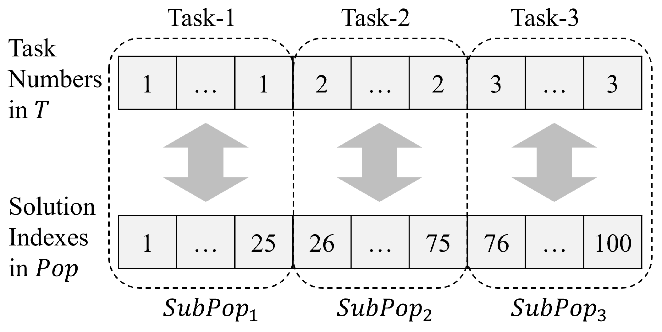
- First, a dynamic multi-task mechanism is designed and combined with the decomposition-based MOEA framework, which assigns multiple evolutionary search tasks for different subpopulations within the entire population and then conditionally merges them into a single task or an integrated population as the evolutionary process goes on, for tackling the large-scale bi-objective feature selection in a more effective way.
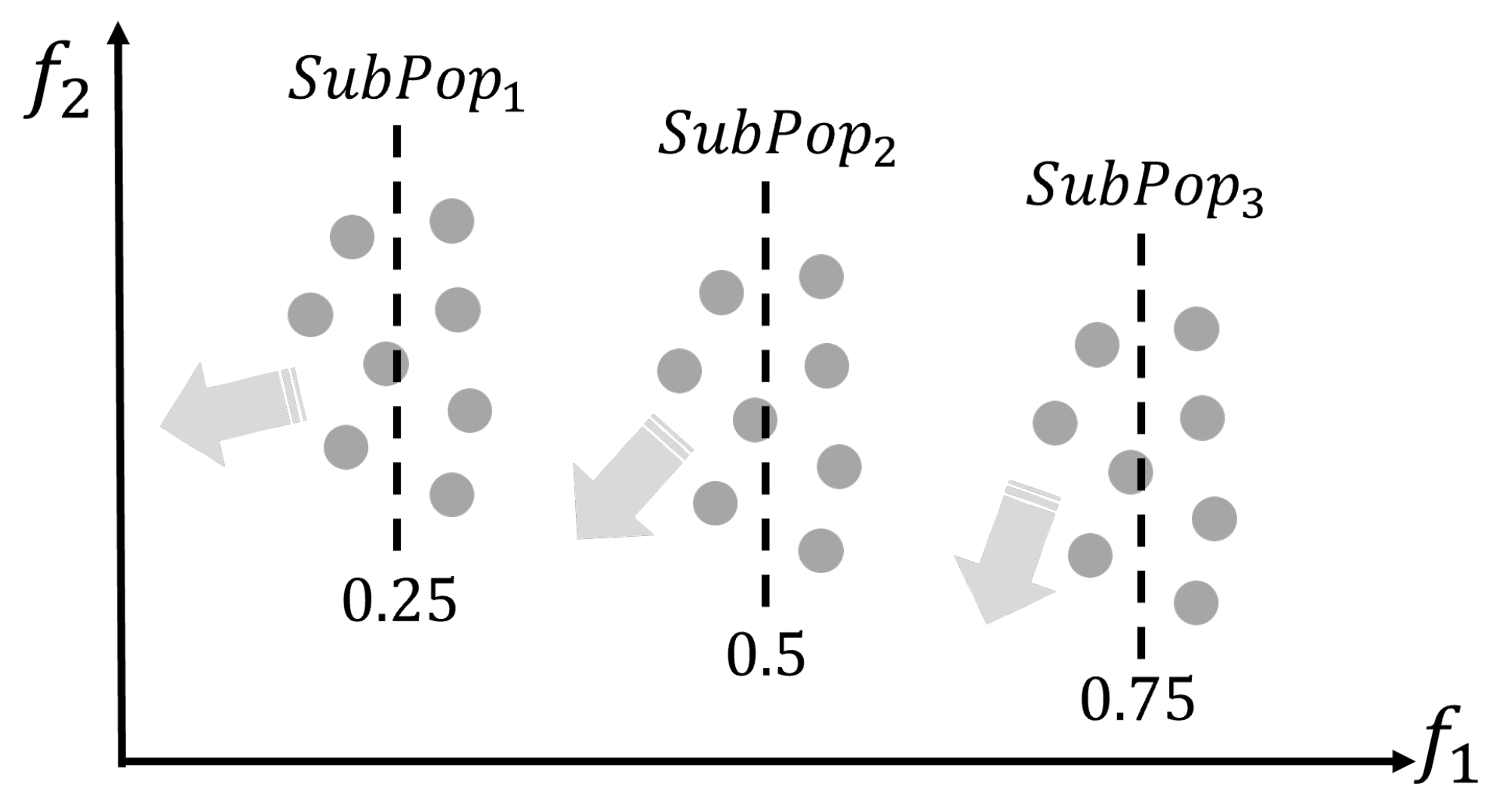
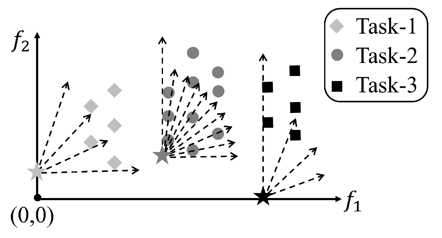
- Second, an adaptive decomposition-based MOEA framework is set up, which cooperates with the above multi-task mechanism via adaptively adjusting the ideal point for each subpopulation related to different tasks, so that each task has distinct search biases and focuses its computational resources on searching more productive areas in the objective space.
- Third, a series of comprehensive studies were conducted in experiments to analyze the optimization and classification performance of the proposed MTDEA algorithm against other state-of-the-art MOEAs, in terms of multiple indicators and using a variety of high-dimensional classification datasets.
2. Related Works
2.1. Bi-Objective Feature Selection Problem
2.2. Evolutionary Feature Selection Methods
2.3. Decomposition-Based MOEA Approaches
3. Proposed Algorithm
3.1. General Framework
3.2. Initialization Process
| Algorithm 1 |
|
| Algorithm 2 |
|
| Algorithm 3 |
|
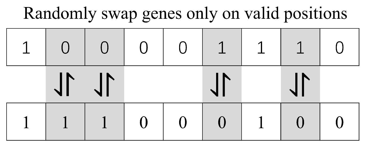
3.3. Reproduction Process
| Algorithm 4 |
|
3.4. Environmental Selection Process
| Algorithm 5 |
|
3.5. Task Merging Process
| Algorithm 6 |
|
4. Experimental Setups
4.1. Classification Datasets
4.2. Comparison Algorithms
4.3. Performance Indicators
4.4. Parameter Settings
5. Experimental Studies
5.1. General Performance Studies
5.2. Nondominated Solution Distributions
5.3. Component Contribution Analyses
5.4. Computational Time Analyses
6. Conclusions
Author Contributions
Funding
Data Availability Statement
Acknowledgments
Conflicts of Interest
References
- Eiben, A.E.; Smith, J.E. What is an evolutionary algorithm? In Introduction to Evolutionary Computing; Springer: Berlin/Heidelberg, Germany, 2015; pp. 25–48. [Google Scholar]
- Coello, C.A.C.; Lamont, G.B.; Van Veldhuizen, D.A. Evolutionary Algorithms for Solving Multi-Objective Problems; Springer: New York, NY, USA, 2007; Volume 5. [Google Scholar]
- Zhou, A.; Qu, B.Y.; Li, H.; Zhao, S.Z.; Suganthan, P.N.; Zhang, Q. Multiobjective evolutionary algorithms: A survey of the state of the art. Swarm Evol. Comput. 2011, 1, 32–49. [Google Scholar] [CrossRef]
- Holland, J.H. Adaptation in Natural and Artificial Systems: An Introductory Analysis with Applications to Biology, Control, and Artificial Intelligence; MIT Press: Cambridge, MA, USA, 1992. [Google Scholar]
- Srinivas, N.; Deb, K. Muiltiobjective optimization using nondominated sorting in genetic algorithms. Evol. Comput. 1994, 2, 221–248. [Google Scholar] [CrossRef]
- Deb, K.; Jain, H. An Evolutionary Many-Objective Optimization Algorithm Using Reference-Point-Based Nondominated Sorting Approach, Part I: Solving Problems With Box Constraints. IEEE Trans. Evol. Comput. 2014, 18, 577–601. [Google Scholar] [CrossRef]
- Castillo, J.C.; Segura, C.; Coello, C.A.C. VSD-MOEA: A Dominance-Based Multiobjective Evolutionary Algorithm with Explicit Variable Space Diversity Management. Evol. Comput. 2022, 30, 195–219. [Google Scholar] [CrossRef] [PubMed]
- Tian, Y.; Cheng, R.; Zhang, X.; Su, Y.; Jin, Y. A Strengthened Dominance Relation Considering Convergence and Diversity for Evolutionary Many-Objective Optimization. IEEE Trans. Evol. Comput. 2019, 23, 331–345. [Google Scholar] [CrossRef]
- Li, H.; Zhang, Q. Multiobjective Optimization Problems with Complicated Pareto Sets, MOEA/D and NSGA-II. IEEE Trans. Evol. Comput. 2009, 13, 284–302. [Google Scholar] [CrossRef]
- Ganesh, N.; Shankar, R.; Kalita, K.; Jangir, P.; Oliva, D.; Pérez-Cisneros, M. A Novel Decomposition-Based Multi-Objective Symbiotic Organism Search Optimization Algorithm. Mathematics 2023, 11, 1898. [Google Scholar] [CrossRef]
- Xu, H.; Zeng, W.; Zhang, D.; Zeng, X. MOEA/HD: A Multiobjective Evolutionary Algorithm Based on Hierarchical Decomposition. IEEE Trans. Cybern. 2019, 49, 517–526. [Google Scholar] [CrossRef] [PubMed]
- Montero, E.; Zapotecas-Martínez, S. An Analysis of Parameters of Decomposition-Based MOEAs on Many-Objective Optimization. In Proceedings of the 2018 IEEE Congress on Evolutionary Computation (CEC), Rio de Janeiro, Brazil, 8–13 July 2018; pp. 1–8. [Google Scholar] [CrossRef]
- Nojima, Y.; Arahari, K.; Takemura, S.; Ishibuchi, H. Multiobjective fuzzy genetics-based machine learning based on MOEA/D with its modifications. In Proceedings of the 2017 IEEE International Conference on Fuzzy Systems (FUZZ-IEEE), Naples, Italy, 9–12 July 2017; pp. 1–6. [Google Scholar] [CrossRef]
- Xu, H.; Zeng, W.; Zeng, X.; Yen, G.G. An Evolutionary Algorithm Based on Minkowski Distance for Many-Objective Optimization. IEEE Trans. Cybern. 2019, 49, 3968–3979. [Google Scholar] [CrossRef]
- Menchaca-Mendez, A.; Coello, C.A.C. GDE-MOEA: A new MOEA based on the generational distance indicator and ɛ-dominance. In Proceedings of the 2015 IEEE Congress on Evolutionary Computation (CEC), Sendai, Japan, 25–28 May 2015; pp. 947–955. [Google Scholar] [CrossRef]
- Xu, H.; Zeng, W.; Zeng, X.; Yen, G.G. A Polar-Metric-Based Evolutionary Algorithm. IEEE Trans. Cybern. 2021, 51, 3429–3440. [Google Scholar] [CrossRef]
- Lopes, C.L.d.V.; Martins, F.V.C.; Wanner, E.F.; Deb, K. Analyzing Dominance Move (MIP-DoM) Indicator for Multiobjective and Many-Objective Optimization. IEEE Trans. Evol. Comput. 2022, 26, 476–489. [Google Scholar] [CrossRef]
- Wang, H.; Jin, Y.; Sun, C.; Doherty, J. Offline data-driven evolutionary optimization using selective surrogate ensembles. IEEE Trans. Evol. Comput. 2018, 23, 203–216. [Google Scholar] [CrossRef]
- Lin, Q.; Wu, X.; Ma, L.; Li, J.; Gong, M.; Coello, C.A.C. An Ensemble Surrogate-Based Framework for Expensive Multiobjective Evolutionary Optimization. IEEE Trans. Evol. Comput. 2022, 26, 631–645. [Google Scholar] [CrossRef]
- Sonoda, T.; Nakata, M. Multiple Classifiers-Assisted Evolutionary Algorithm Based on Decomposition for High-Dimensional Multiobjective Problems. IEEE Trans. Evol. Comput. 2022, 26, 1581–1595. [Google Scholar] [CrossRef]
- Goh, C.K.; Tan, K.C. A competitive-cooperative coevolutionary paradigm for dynamic multiobjective optimization. IEEE Trans. Evol. Comput. 2008, 13, 103–127. [Google Scholar]
- Zhan, Z.H.; Li, J.; Cao, J.; Zhang, J.; Chung, H.S.H.; Shi, Y.H. Multiple Populations for Multiple Objectives: A Coevolutionary Technique for Solving Multiobjective Optimization Problems. IEEE Trans. Cybern. 2013, 43, 445–463. [Google Scholar] [CrossRef] [PubMed]
- Ma, X.; Li, X.; Zhang, Q.; Tang, K.; Liang, Z.; Xie, W.; Zhu, Z. A survey on cooperative co-evolutionary algorithms. IEEE Trans. Evol. Comput. 2018, 23, 421–441. [Google Scholar] [CrossRef]
- Da, B.; Gupta, A.; Ong, Y.S.; Feng, L. Evolutionary multitasking across single and multi-objective formulations for improved problem solving. In Proceedings of the 2016 IEEE Congress on Evolutionary Computation (CEC), Vancouver, BC, Canada, 24–29 July 2016; pp. 1695–1701. [Google Scholar]
- Gupta, A.; Ong, Y.S.; Feng, L.; Tan, K.C. Multiobjective Multifactorial Optimization in Evolutionary Multitasking. IEEE Trans. Cybern. 2017, 47, 1652–1665. [Google Scholar] [CrossRef]
- Rauniyar, A.; Nath, R.; Muhuri, P.K. Multi-factorial evolutionary algorithm based novel solution approach for multi-objective pollution-routing problem. Comput. Ind. Eng. 2019, 130, 757–771. [Google Scholar] [CrossRef]
- Palakonda, V.; Mallipeddi, R. An Evolutionary Algorithm for Multi and Many-Objective Optimization with Adaptive Mating and Environmental Selection. IEEE Access 2020, 8, 82781–82796. [Google Scholar] [CrossRef]
- Park, J.; Ajani, O.S.; Mallipeddi, R. Optimization-Based Energy Disaggregation: A Constrained Multi-Objective Approach. Mathematics 2023, 11, 563. [Google Scholar] [CrossRef]
- Ríos, A.; Hernández, E.E.; Valdez, S.I. A Two-Stage Mono- and Multi-Objective Method for the Optimization of General UPS Parallel Manipulators. Mathematics 2021, 9, 543. [Google Scholar] [CrossRef]
- Leung, M.F.; Coello, C.A.C.; Cheung, C.C.; Ng, S.C.; Lui, A.K.F. A Hybrid Leader Selection Strategy for Many-Objective Particle Swarm Optimization. IEEE Access 2020, 8, 189527–189545. [Google Scholar] [CrossRef]
- Cao, F.; Tang, Z.; Zhu, C.; Zhao, X. An Efficient Hybrid Multi-Objective Optimization Method Coupling Global Evolutionary and Local Gradient Searches for Solving Aerodynamic Optimization Problems. Mathematics 2023, 11, 3844. [Google Scholar] [CrossRef]
- Garces-Jimenez, A.; Gomez-Pulido, J.M.; Gallego-Salvador, N.; Garcia-Tejedor, A.J. Genetic and Swarm Algorithms for Optimizing the Control of Building HVAC Systems Using Real Data: A Comparative Study. Mathematics 2021, 9, 2181. [Google Scholar] [CrossRef]
- Ramos-Pérez, J.M.; Miranda, G.; Segredo, E.; León, C.; Rodríguez-León, C. Application of Multi-Objective Evolutionary Algorithms for Planning Healthy and Balanced School Lunches. Mathematics 2021, 9, 80. [Google Scholar] [CrossRef]
- Cai, H.; Lin, Q.; Liu, H.; Li, X.; Xiao, H. A Multi-Objective Optimisation Mathematical Model with Constraints Conducive to the Healthy Rhythm for Lighting Control Strategy. Mathematics 2022, 10, 3471. [Google Scholar] [CrossRef]
- Alshammari, N.F.; Samy, M.M.; Barakat, S. Comprehensive Analysis of Multi-Objective Optimization Algorithms for Sustainable Hybrid Electric Vehicle Charging Systems. Mathematics 2023, 11, 1741. [Google Scholar] [CrossRef]
- Zhu, W.; Li, H.; Wei, W. A Two-Stage Multi-Objective Evolutionary Algorithm for Community Detection in Complex Networks. Mathematics 2023, 11, 2702. [Google Scholar] [CrossRef]
- Gao, C.; Yin, Z.; Wang, Z.; Li, X.; Li, X. Multilayer Network Community Detection: A Novel Multi-Objective Evolutionary Algorithm Based on Consensus Prior Information [Feature]. IEEE Comput. Intell. Mag. 2023, 18, 46–59. [Google Scholar] [CrossRef]
- Xue, Y.; Chen, C.; S?owik, A. Neural Architecture Search Based on a Multi-Objective Evolutionary Algorithm with Probability Stack. IEEE Trans. Evol. Comput. 2023, 27, 778–786. [Google Scholar] [CrossRef]
- Ponti, A.; Candelieri, A.; Giordani, I.; Archetti, F. Intrusion Detection in Networks by Wasserstein Enabled Many-Objective Evolutionary Algorithms. Mathematics 2023, 11, 2342. [Google Scholar] [CrossRef]
- Othman, R.A.; Darwish, S.M.; Abd El-Moghith, I.A. A Multi-Objective Crowding Optimization Solution for Efficient Sensing as a Service in Virtualized Wireless Sensor Networks. Mathematics 2023, 11, 1128. [Google Scholar] [CrossRef]
- Long, S.; Zhang, Y.; Deng, Q.; Pei, T.; Ouyang, J.; Xia, Z. An Efficient Task Offloading Approach Based on Multi-Objective Evolutionary Algorithm in Cloud-Edge Collaborative Environment. IEEE Trans. Netw. Sci. Eng. 2023, 10, 645–657. [Google Scholar] [CrossRef]
- Zhang, Z.; Ma, S.; Jiang, X. Research on Multi-Objective Multi-Robot Task Allocation by Lin-Kernighan-Helsgaun Guided Evolutionary Algorithms. Mathematics 2022, 10, 4714. [Google Scholar] [CrossRef]
- Nguyen, B.H.; Xue, B.; Andreae, P.; Ishibuchi, H.; Zhang, M. Multiple Reference Points-Based Decomposition for Multiobjective Feature Selection in Classification: Static and Dynamic Mechanisms. IEEE Trans. Evol. Comput. 2020, 24, 170–184. [Google Scholar] [CrossRef]
- Xu, H.; Huang, C.; Wen, H.; Yan, T.; Lin, Y.; Xie, Y. A Hybrid Initialization and Effective Reproduction-Based Evolutionary Algorithm for Tackling Bi-Objective Large-Scale Feature Selection in Classification. Mathematics 2024, 12, 554. [Google Scholar] [CrossRef]
- Dash, M.; Liu, H. Feature selection for classification. Intell. Data Anal. 1997, 1, 131–156. [Google Scholar] [CrossRef]
- Xu, H.; Xue, B.; Zhang, M. Segmented Initialization and Offspring Modification in Evolutionary Algorithms for Bi-Objective Feature Selection. In Proceedings of the 2020 Genetic and Evolutionary Computation Conference, New York, NY, USA, 8–12 July 2020; pp. 444–452. [Google Scholar]
- Zille, H.; Mostaghim, S. Comparison study of large-scale optimisation techniques on the LSMOP benchmark functions. In Proceedings of the 2017 IEEE Symposium Series on Computational Intelligence (SSCI), Honolulu, HI, USA, 27 November–1 December 2017; pp. 1–8. [Google Scholar]
- Ma, X.; Liu, F.; Qi, Y.; Wang, X.; Li, L.; Jiao, L.; Yin, M.; Gong, M. A Multiobjective Evolutionary Algorithm Based on Decision Variable Analyses for Multiobjective Optimization Problems With Large-Scale Variables. IEEE Trans. Evol. Comput. 2016, 20, 275–298. [Google Scholar] [CrossRef]
- Zhang, X.; Tian, Y.; Cheng, R.; Jin, Y. A Decision Variable Clustering-Based Evolutionary Algorithm for Large-Scale Many-Objective Optimization. IEEE Trans. Evol. Comput. 2018, 22, 97–112. [Google Scholar] [CrossRef]
- Bai, H.; Cheng, R.; Yazdani, D.; Tan, K.C.; Jin, Y. Evolutionary Large-Scale Dynamic Optimization Using Bilevel Variable Grouping. IEEE Trans. Cybern. 2022, 53, 6937–6950. [Google Scholar] [CrossRef] [PubMed]
- Yang, X.; Zou, J.; Yang, S.; Zheng, J.; Liu, Y. A Fuzzy Decision Variables Framework for Large-Scale Multiobjective Optimization. IEEE Trans. Evol. Comput. 2023, 27, 445–459. [Google Scholar] [CrossRef]
- Ma, X.; Zheng, Y.; Zhu, Z.; Li, X.; Wang, L.; Qi, Y.; Yang, J. Improving Evolutionary Multitasking Optimization by Leveraging Inter-Task Gene Similarity and Mirror Transformation. IEEE Comput. Intell. Mag. 2021, 16, 38–53. [Google Scholar] [CrossRef]
- Ming, F.; Gong, W.; Gao, L. Adaptive Auxiliary Task Selection for Multitasking-Assisted Constrained Multi-Objective Optimization [Feature]. IEEE Comput. Intell. Mag. 2023, 18, 18–30. [Google Scholar] [CrossRef]
- Liang, Z.; Liang, W.; Wang, Z.; Ma, X.; Liu, L.; Zhu, Z. Multiobjective Evolutionary Multitasking with Two-Stage Adaptive Knowledge Transfer Based on Population Distribution. IEEE Trans. Syst. Man, Cybern. Syst. 2022, 52, 4457–4469. [Google Scholar] [CrossRef]
- Feng, Y.; Feng, L.; Kwong, S.; Tan, K.C. A Multivariation Multifactorial Evolutionary Algorithm for Large-Scale Multiobjective Optimization. IEEE Trans. Evol. Comput. 2022, 26, 248–262. [Google Scholar] [CrossRef]
- Gao, W.; Cheng, J.; Gong, M.; Li, H.; Xie, J. Multiobjective Multitasking Optimization with Subspace Distribution Alignment and Decision Variable Transfer. IEEE Trans. Emerg. Top. Comput. Intell. 2022, 6, 818–827. [Google Scholar] [CrossRef]
- Li, J.; Cheng, K.; Wang, S.; Morstatter, F.; Trevino, R.P.; Tang, J.; Liu, H. Feature selection: A data perspective. ACM Comput. Surv. (CSUR) 2017, 50, 1–45. [Google Scholar] [CrossRef]
- De La Iglesia, B. Evolutionary computation for feature selection in classification problems. Wiley Interdiscip. Rev. Data Min. Knowl. Discov. 2013, 3, 381–407. [Google Scholar] [CrossRef]
- Xue, B.; Zhang, M.; Browne, W.N.; Yao, X. A survey on evolutionary computation approaches to feature selection. IEEE Trans. Evol. Comput. 2015, 20, 606–626. [Google Scholar] [CrossRef]
- Dokeroglu, T.; Deniz, A.; Kiziloz, H.E. A comprehensive survey on recent metaheuristics for feature selection. Neurocomputing 2022, 494, 269–296. [Google Scholar] [CrossRef]
- Mukhopadhyay, A.; Maulik, U. An SVM-wrapped multiobjective evolutionary feature selection approach for identifying cancer-microRNA markers. IEEE Trans. Nanobiosci. 2013, 12, 275–281. [Google Scholar] [CrossRef] [PubMed]
- Vignolo, L.D.; Milone, D.H.; Scharcanski, J. Feature selection for face recognition based on multi-objective evolutionary wrappers. Expert Syst. Appl. 2013, 40, 5077–5084. [Google Scholar] [CrossRef]
- Guyon, I.; Elisseeff, A. An introduction to variable and feature selection. J. Mach. Learn. Res. 2003, 3, 1157–1182. [Google Scholar]
- Lazar, C.; Taminau, J.; Meganck, S.; Steenhoff, D.; Coletta, A.; Molter, C.; de Schaetzen, V.; Duque, R.; Bersini, H.; Nowe, A. A survey on filter techniques for feature selection in gene expression microarray analysis. IEEE/ACM Trans. Comput. Biol. Bioinform. (TCBB) 2012, 9, 1106–1119. [Google Scholar] [CrossRef] [PubMed]
- Xue, B.; Cervante, L.; Shang, L.; Browne, W.N.; Zhang, M. Multi-objective evolutionary algorithms for filter based feature selection in classification. Int. J. Artif. Intell. Tools 2013, 22, 1350024. [Google Scholar] [CrossRef]
- Xue, B.; Zhang, M.; Browne, W.N. Particle swarm optimisation for feature selection in classification: Novel initialisation and updating mechanisms. Appl. Soft Comput. 2014, 18, 261–276. [Google Scholar] [CrossRef]
- Chen, K.; Xue, B.; Zhang, M.; Zhou, F. Evolutionary Multitasking for Feature Selection in High-Dimensional Classification via Particle Swarm Optimization. IEEE Trans. Evol. Comput. 2022, 26, 446–460. [Google Scholar] [CrossRef]
- Chen, K.; Xue, B.; Zhang, M.; Zhou, F. An Evolutionary Multitasking-Based Feature Selection Method for High-Dimensional Classification. IEEE Trans. Cybern. 2022, 52, 7172–7186. [Google Scholar] [CrossRef]
- Cheng, F.; Cui, J.; Wang, Q.; Zhang, L. A Variable Granularity Search-Based Multiobjective Feature Selection Algorithm for High-Dimensional Data Classification. IEEE Trans. Evol. Comput. 2023, 27, 266–280. [Google Scholar] [CrossRef]
- Tian, Y.; Zhang, X.; Wang, C.; Jin, Y. An Evolutionary Algorithm for Large-Scale Sparse Multiobjective Optimization Problems. IEEE Trans. Evol. Comput. 2020, 24, 380–393. [Google Scholar] [CrossRef]
- Xu, H.; Xue, B.; Zhang, M. A Duplication Analysis-Based Evolutionary Algorithm for Biobjective Feature Selection. IEEE Trans. Evol. Comput. 2021, 25, 205–218. [Google Scholar] [CrossRef]
- Jiao, R.; Xue, B.; Zhang, M. Solving Multi-objective Feature Selection Problems in Classification via Problem Reformulation and Duplication Handling. IEEE Trans. Evol. Comput. 2022, 1, 1. [Google Scholar] [CrossRef]
- Cheng, F.; Chu, F.; Xu, Y.; Zhang, L. A Steering-Matrix-Based Multiobjective Evolutionary Algorithm for High-Dimensional Feature Selection. IEEE Trans. Cybern. 2022, 52, 9695–9708. [Google Scholar] [CrossRef] [PubMed]
- Li, H.; Zhang, Q. A multiobjective differential evolution based on decomposition for multiobjective optimization with variable linkages. In Proceedings of the International Conference on Parallel Problem Solving from Nature, Reykjavik, Iceland, 9–13 September 2006; Springer: Berlin/Heidelberg, Germany, 2006; pp. 583–592. [Google Scholar]
- Yang, S.; Huang, H.; Luo, F.; Xu, Y.; Hao, Z. Local-Diversity Evaluation Assignment Strategy for Decomposition-Based Multiobjective Evolutionary Algorithm. IEEE Trans. Syst. Man, Cybern. Syst. 2023, 53, 1697–1709. [Google Scholar] [CrossRef]
- He, L.; Shang, K.; Nan, Y.; Ishibuchi, H.; Srinivasan, D. Relation Between Objective Space Normalization and Weight Vector Scaling in Decomposition-Based Multiobjective Evolutionary Algorithms. IEEE Trans. Evol. Comput. 2023, 27, 1177–1191. [Google Scholar] [CrossRef]
- Zhao, Q.; Guo, Y.; Yao, X.; Gong, D. Decomposition-Based Multiobjective Optimization Algorithms with Adaptively Adjusting Weight Vectors and Neighborhoods. IEEE Trans. Evol. Comput. 2023, 27, 1485–1497. [Google Scholar] [CrossRef]
- Pang, L.M.; Ishibuchi, H.; Shang, K. Use of Two Penalty Values in Multiobjective Evolutionary Algorithm Based on Decomposition. IEEE Trans. Cybern. 2023, 53, 7174–7186. [Google Scholar] [CrossRef]
- Wang, R.; Zhang, Q.; Zhang, T. Decomposition-Based Algorithms Using Pareto Adaptive Scalarizing Methods. IEEE Trans. Evol. Comput. 2016, 20, 821–837. [Google Scholar] [CrossRef]
- Zhang, Q.; Li, H. MOEA/D: A Multiobjective Evolutionary Algorithm Based on Decomposition. IEEE Trans. Evol. Comput. 2007, 11, 712–731. [Google Scholar] [CrossRef]
- Zhang, Q.; Liu, W.; Li, H. The performance of a new version of MOEA/D on CEC09 unconstrained MOP test instances. In Proceedings of the 2009 IEEE Congress on Evolutionary Computation, Trondheim, Norway, 18–21 May 2009; pp. 203–208. [Google Scholar] [CrossRef]
- Li, K.; Deb, K.; Zhang, Q.; Kwong, S. An Evolutionary Many-Objective Optimization Algorithm Based on Dominance and Decomposition. IEEE Trans. Evol. Comput. 2015, 19, 694–716. [Google Scholar] [CrossRef]
- Qi, Y.; Ma, X.; Liu, F.; Jiao, L.; Sun, J.; Wu, J. MOEA/D with Adaptive Weight Adjustment. Evol. Comput. 2014, 22, 231–264. [Google Scholar] [CrossRef]
- Dua, D.; Graff, C. UCI Machine Learning Repository. 2017. Available online: https://archive.ics.uci.edu/datasets (accessed on 12 April 2024).
- Deb, K.; Pratap, A.; Agarwal, S.; Meyarivan, T. A fast and elitist multiobjective genetic algorithm: NSGA-II. IEEE Trans. Evol. Comput. 2002, 6, 182–197. [Google Scholar] [CrossRef]
- While, L.; Hingston, P.; Barone, L.; Huband, S. A faster algorithm for calculating Hypervolume. IEEE Trans. Evol. Comput. 2006, 10, 29–38. [Google Scholar] [CrossRef]
- Tian, Y.; Cheng, R.; Zhang, X.; Jin, Y. PlatEMO: A MATLAB Platform for Evolutionary Multi-Objective Optimization. IEEE Comput. Intell. Mag. 2017, 12, 73–87. [Google Scholar] [CrossRef]
- Tran, B.; Xue, B.; Zhang, M.; Nguyen, S. Investigation on particle swarm optimisation for feature selection on high-dimensional data: Local search and selection bias. Connect. Sci. 2016, 28, 270–294. [Google Scholar] [CrossRef]


| No. | Dataset | Feature | Sample | Class |
|---|---|---|---|---|
| 1 | ORL | 1024 | 400 | 40 |
| 2 | Yale | 1024 | 165 | 15 |
| 3 | Colon | 2000 | 62 | 2 |
| 4 | SRBCT | 2308 | 83 | 4 |
| 5 | AR10P | 2400 | 130 | 10 |
| 6 | PIE10P | 2420 | 210 | 10 |
| 7 | Lymphoma | 4026 | 96 | 9 |
| 9 | DLBCL | 5469 | 77 | 2 |
| 8 | TOX171 | 5748 | 171 | 4 |
| 10 | Brain1 | 5920 | 90 | 5 |
| 11 | Leukemia | 7070 | 72 | 2 |
| 12 | CNS | 7129 | 60 | 2 |
| 13 | ALLAML | 7129 | 72 | 2 |
| 14 | Carcinom | 9182 | 174 | 11 |
| 15 | Nci9 | 9712 | 60 | 9 |
| 16 | Arcene | 10,000 | 200 | 2 |
| 17 | Pixraw10P | 10,000 | 100 | 10 |
| 18 | Orlraws10P | 10,304 | 100 | 10 |
| 19 | Brain2 | 10,367 | 50 | 4 |
| 20 | Prostate | 10,509 | 102 | 2 |
| Metric | MTDEA | NSGA-II | MOEA/D | MOEA/AWA | MOEA/HD | SparseEA | DAEA | PRDH |
|---|---|---|---|---|---|---|---|---|
| HV | 1.012 | 5.215 | 3.917 | 5.290 | 6.275 | 7.530 | 2.192 | 4.567 |
| MCE | 3.615 | 4.688 | 5.124 | 4.787 | 5.030 | 4.303 | 3.740 | 4.714 |
| NSF | 1.000 | 5.270 | 3.112 | 5.640 | 6.461 | 7.949 | 2.110 | 4.457 |
| Dataset | MTDEA | NSGA-II | MOEA/D | MOEA/AWA | MOEA/HD | SparseEA | DAEA | PRDH |
|---|---|---|---|---|---|---|---|---|
| ORL | 7.928e-01 | 6.103e-01 | 6.642e-01 | 6.576e-01 | 5.996e-01 | 5.859e-01 | 7.249e-01 | 6.350e-01 |
| ±1.80e-02 | ±1.08e-02 | ±1.53e-02 | ±1.79e-02 | ±1.25e-02 | ±9.94e-03 | ±1.75e-02 | ±1.18e-02 | |
| Yale | 6.597e-01 | 4.878e-01 | 5.127e-01 | 5.199e-01 | 4.920e-01 | 4.811e-01 | 6.050e-01 | 5.071e-01 |
| ±3.18e-02 | ±1.34e-02 | ±2.62e-02 | ±2.40e-02 | ±3.39e-02 | ±1.64e-02 | ±2.48e-02 | ±2.15e-02 | |
| Colon | 7.746e-01 | 5.500e-01 | 6.078e-01 | 5.466e-01 | 5.239e-01 | 4.987e-01 | 6.680e-01 | 5.554e-01 |
| ±3.84e-02 | ±2.65e-02 | ±4.78e-02 | ±3.55e-02 | ±3.30e-02 | ±2.01e-02 | ±3.95e-02 | ±3.10e-02 | |
| SRBCT | 6.654e-01 | 2.841e-01 | 3.178e-01 | 2.983e-01 | 2.554e-01 | 2.479e-01 | 3.028e-01 | 2.768e-01 |
| ±1.70e-01 | ±2.05e-03 | ±2.03e-03 | ±2.74e-03 | ±1.81e-03 | ±1.69e-03 | ±1.96e-02 | ±3.17e-03 | |
| AR10P | 4.972e-01 | 3.631e-01 | 3.709e-01 | 3.544e-01 | 3.449e-01 | 3.223e-01 | 4.314e-01 | 3.603e-01 |
| ±2.74e-02 | ±2.01e-02 | ±2.26e-02 | ±1.35e-02 | ±1.75e-02 | ±1.11e-02 | ±2.05e-02 | ±1.86e-02 | |
| PIE10P | 8.127e-01 | 6.023e-01 | 6.458e-01 | 6.003e-01 | 5.883e-01 | 5.434e-01 | 6.982e-01 | 6.056e-01 |
| ±2.00e-02 | ±1.06e-02 | ±1.13e-02 | ±1.29e-02 | ±1.22e-02 | ±6.44e-03 | ±1.57e-02 | ±9.92e-03 | |
| Lymphoma | 7.645e-01 | 5.603e-01 | 6.007e-01 | 5.598e-01 | 5.456e-01 | 5.067e-01 | 6.434e-01 | 5.626e-01 |
| ±2.18e-02 | ±9.91e-03 | ±9.76e-03 | ±1.59e-02 | ±8.85e-03 | ±1.07e-02 | ±1.57e-02 | ±6.99e-03 | |
| TOX171 | 6.749e-01 | 4.829e-01 | 4.876e-01 | 4.697e-01 | 4.776e-01 | 4.575e-01 | 5.423e-01 | 4.907e-01 |
| ±2.21e-02 | ±8.58e-03 | ±1.97e-02 | ±1.13e-02 | ±1.65e-02 | ±1.19e-02 | ±1.92e-02 | ±1.23e-02 | |
| DLBCL | 8.054e-01 | 5.852e-01 | 5.999e-01 | 5.722e-01 | 5.735e-01 | 5.469e-01 | 6.703e-01 | 5.982e-01 |
| ±3.06e-02 | ±2.02e-02 | ±1.82e-02 | ±2.17e-02 | ±1.67e-02 | ±1.83e-02 | ±2.12e-02 | ±1.77e-02 | |
| Brain1 | 6.496e-01 | 4.718e-01 | 4.906e-01 | 4.657e-01 | 4.535e-01 | 4.312e-01 | 5.127e-01 | 4.744e-01 |
| ±1.38e-02 | ±3.11e-03 | ±1.09e-02 | ±1.06e-02 | ±1.00e-02 | ±1.78e-03 | ±8.53e-03 | ±2.57e-03 | |
| Leukemia | 7.626e-01 | 5.360e-01 | 5.450e-01 | 5.295e-01 | 5.126e-01 | 4.972e-01 | 6.022e-01 | 5.454e-01 |
| ±2.70e-02 | ±8.95e-03 | ±1.94e-02 | ±1.89e-02 | ±1.79e-02 | ±9.84e-03 | ±1.67e-02 | ±2.04e-02 | |
| CNS | 5.255e-01 | 3.781e-01 | 3.743e-01 | 3.690e-01 | 3.707e-01 | 3.669e-01 | 4.408e-01 | 3.844e-01 |
| ±5.88e-02 | ±3.28e-02 | ±3.32e-02 | ±3.09e-02 | ±3.25e-02 | ±1.57e-02 | ±3.03e-02 | ±2.94e-02 | |
| ALLAML | 7.278e-01 | 5.205e-01 | 5.358e-01 | 5.084e-01 | 5.060e-01 | 4.853e-01 | 5.826e-01 | 5.280e-01 |
| ±2.93e-02 | ±1.52e-02 | ±1.34e-02 | ±1.60e-02 | ±1.44e-02 | ±1.52e-02 | ±1.83e-02 | ±1.32e-02 | |
| Carcinom | 7.199e-01 | 5.180e-01 | 5.233e-01 | 5.098e-01 | 5.091e-01 | 4.871e-01 | 5.809e-01 | 5.193e-01 |
| ±1.40e-02 | ±1.09e-02 | ±1.55e-02 | ±1.00e-02 | ±1.10e-02 | ±8.18e-03 | ±1.18e-02 | ±7.20e-03 | |
| Nci9 | 3.570e-01 | 2.406e-01 | 2.616e-01 | 2.544e-01 | 2.370e-01 | 2.254e-01 | 2.707e-01 | 2.451e-01 |
| ±2.33e-02 | ±2.54e-02 | ±2.94e-02 | ±2.80e-02 | ±2.21e-02 | ±2.00e-02 | ±2.75e-02 | ±2.71e-02 | |
| Arcene | 5.132e-01 | 3.625e-01 | 3.724e-01 | 3.649e-01 | 3.445e-01 | 3.374e-01 | 3.859e-01 | 3.647e-01 |
| ±4.15e-03 | ±1.10e-03 | ±1.85e-03 | ±2.23e-03 | ±1.24e-03 | ±1.29e-03 | ±2.75e-03 | ±1.71e-03 | |
| Pixraw10P | 8.104e-01 | 5.795e-01 | 5.911e-01 | 5.773e-01 | 5.640e-01 | 5.407e-01 | 6.327e-01 | 5.846e-01 |
| ±6.33e-03 | ±2.22e-03 | ±9.88e-03 | ±7.09e-03 | ±7.64e-03 | ±1.57e-03 | ±9.37e-03 | ±2.65e-03 | |
| Orlraws10P | 7.491e-01 | 5.390e-01 | 5.447e-01 | 5.328e-01 | 5.297e-01 | 5.057e-01 | 5.951e-01 | 5.444e-01 |
| ±1.43e-02 | ±7.53e-03 | ±9.58e-03 | ±1.13e-02 | ±8.00e-03 | ±3.88e-03 | ±8.65e-03 | ±4.77e-03 | |
| Brain2 | 5.603e-01 | 3.903e-01 | 3.824e-01 | 3.816e-01 | 3.782e-01 | 3.687e-01 | 4.335e-01 | 3.898e-01 |
| ±2.84e-02 | ±2.15e-02 | ±2.43e-02 | ±2.91e-02 | ±2.12e-02 | ±1.66e-02 | ±2.82e-02 | ±1.83e-02 | |
| Prostate | 6.456e-01 | 4.629e-01 | 4.599e-01 | 4.574e-01 | 4.559e-01 | 4.419e-01 | 5.204e-01 | 4.693e-01 |
| ±2.38e-02 | ±1.29e-02 | ±1.51e-02 | ±1.58e-02 | ±1.16e-02 | ±8.71e-03 | ±1.53e-02 | ±1.52e-02 |
| Dataset | MTDEA | NSGA-II | MOEA/D | MOEA/AWA | MOEA/HD | SparseEA | DAEA | PRDH |
|---|---|---|---|---|---|---|---|---|
| ORL | 1.375e-01 | ⋆ 1.442e-01 | ⋆ 1.437e-01 | 1.475e-01 | 1.517e-01 | 1.471e-01 | ⋆ 1.304e-01 | 1.487e-01 |
| ±1.49e-02 | ±2.01e-02 | ±1.35e-02 | ±1.30e-02 | ±2.03e-02 | ±1.33e-02 | ±1.49e-02 | ±1.39e-02 | |
| Yale | 2.944e-01 | 3.478e-01 | 3.622e-01 | 3.367e-01 | 3.400e-01 | ⋆ 3.133e-01 | ⋆ 2.989e-01 | 3.500e-01 |
| ±3.60e-02 | ±2.53e-02 | ±3.82e-02 | ±3.90e-02 | ±5.20e-02 | ±2.78e-02 | ±3.01e-02 | ±3.13e-02 | |
| Colon | 1.421e-01 | 2.132e-01 | 2.079e-01 | 2.079e-01 | 2.342e-01 | 1.974e-01 | 1.684e-01 | 2.132e-01 |
| ±4.86e-02 | ±4.35e-02 | ±6.50e-02 | ±5.53e-02 | ±5.26e-02 | ±3.77e-02 | ±5.01e-02 | ±4.97e-02 | |
| SRBCT | 2.840e-01 | 6.400e-01 | 6.400e-01 | 6.400e-01 | 6.400e-01 | 6.400e-01 | 6.400e-01 | 6.400e-01 |
| ±2.15e-01 | ±1.14e-16 | ±1.14e-16 | ±1.14e-16 | ±1.14e-16 | ±1.14e-16 | ±1.14e-16 | ±1.14e-16 | |
| AR10P | 4.688e-01 | ⋆ 4.900e-01 | 5.200e-01 | 4.962e-01 | 5.150e-01 | 5.075e-01 | ⋆ 4.700e-01 | 5.063e-01 |
| ±3.52e-02 | ±3.38e-02 | ±3.77e-02 | ±2.47e-02 | ±3.08e-02 | ±2.00e-02 | ±3.10e-02 | ±3.02e-02 | |
| PIE10P | 7.750e-02 | 9.667e-02 | 1.033e-01 | 9.583e-02 | 1.017e-01 | 1.017e-01 | ⋆ 8.583e-02 | 1.058e-01 |
| ±2.25e-02 | ±1.28e-02 | ±2.27e-02 | ±1.42e-02 | ±1.42e-02 | ±1.07e-02 | ±1.82e-02 | ±1.56e-02 | |
| Lymphoma | 1.200e-01 | 1.350e-01 | ⋆ 1.300e-01 | ⋆ 1.333e-01 | ⋆ 1.300e-01 | ⋆ 1.300e-01 | ⋆ 1.250e-01 | 1.333e-01 |
| ±2.27e-02 | ±1.31e-02 | ±1.49e-02 | ±2.16e-02 | ±1.03e-02 | ±1.84e-02 | ±2.39e-02 | ±1.08e-02 | |
| TOX171 | 2.038e-01 | 2.236e-01 | 2.406e-01 | 2.330e-01 | 2.274e-01 | ⋆ 2.132e-01 | ⋆ 2.179e-01 | 2.208e-01 |
| ±2.97e-02 | ±1.53e-02 | ±3.56e-02 | ±2.06e-02 | ±2.84e-02 | ±2.38e-02 | ±2.84e-02 | ±2.04e-02 | |
| DLBCL | 7.174e-02 | ⋆ 5.870e-02 | ⋆ 7.174e-02 | ⋆ 6.957e-02 | ⋆ 6.304e-02 | 3.913e-02 | 4.130e-02 | 4.130e-02 |
| ±3.80e-02 | ±3.53e-02 | ±2.92e-02 | ±3.28e-02 | ±2.63e-02 | ±3.43e-02 | ±2.98e-02 | ±2.98e-02 | |
| Brain1 | 2.593e-01 | ⋆ 2.593e-01 | ⋆ 2.593e-01 | ⋆ 2.593e-01 | ⋆ 2.593e-01 | ⋆ 2.593e-01 | ⋆ 2.593e-01 | ⋆ 2.593e-01 |
| ±1.20e-02 | ±0.00e+00 | ±0.00e+00 | ±0.00e+00 | ±0.00e+00 | ±0.00e+00 | ±0.00e+00 | ±0.00e+00 | |
| Leukemia | 1.091e-01 | 1.318e-01 | 1.455e-01 | 1.364e-01 | 1.455e-01 | ⋆ 1.273e-01 | ⋆ 1.205e-01 | ⋆ 1.227e-01 |
| ±3.73e-02 | ±1.40e-02 | ±2.80e-02 | ±2.95e-02 | ±2.80e-02 | ±1.87e-02 | ±2.67e-02 | ±3.64e-02 | |
| CNS | 4.000e-01 | ⋆ 4.139e-01 | ⋆ 4.417e-01 | ⋆ 4.167e-01 | ⋆ 4.167e-01 | ⋆ 3.833e-01 | ⋆ 3.833e-01 | ⋆ 4.083e-01 |
| ±7.77e-02 | ±6.11e-02 | ±5.55e-02 | ±6.11e-02 | ±5.84e-02 | ±3.07e-02 | ±4.73e-02 | ±5.49e-02 | |
| ALLAML | 1.455e-01 | ⋆ 1.568e-01 | ⋆ 1.591e-01 | 1.727e-01 | ⋆ 1.636e-01 | ⋆ 1.500e-01 | ⋆ 1.500e-01 | ⋆ 1.523e-01 |
| ±3.79e-02 | ±2.75e-02 | ±2.33e-02 | ±2.80e-02 | ±2.28e-02 | ±2.99e-02 | ±2.60e-02 | ±2.22e-02 | |
| Carcinom | 1.356e-01 | ⋆ 1.423e-01 | 1.500e-01 | ⋆ 1.394e-01 | 1.500e-01 | ⋆ 1.385e-01 | ⋆ 1.327e-01 | 1.471e-01 |
| ±1.59e-02 | ±1.91e-02 | ±2.30e-02 | ±1.51e-02 | ±2.03e-02 | ±1.60e-02 | ±1.64e-02 | ±1.29e-02 | |
| Nci9 | 6.289e-01 | 6.579e-01 | ⋆ 6.342e-01 | ⋆ 6.368e-01 | ⋆ 6.421e-01 | 6.553e-01 | ⋆ 6.316e-01 | ⋆ 6.526e-01 |
| ±3.18e-02 | ±4.68e-02 | ±5.26e-02 | ±5.09e-02 | ±4.39e-02 | ±4.00e-02 | ±4.83e-02 | ±4.95e-02 | |
| Arcene | 4.333e-01 | ⋆ 4.333e-01 | ⋆ 4.333e-01 | ⋆ 4.333e-01 | ⋆ 4.333e-01 | ⋆ 4.333e-01 | ⋆ 4.333e-01 | ⋆ 4.333e-01 |
| ±1.14e-16 | ±1.14e-16 | ±1.14e-16 | ±1.14e-16 | ±1.14e-16 | ±1.14e-16 | ±1.14e-16 | ±1.14e-16 | |
| Pixraw10P | 3.333e-02 | ⋆ 3.333e-02 | ⋆ 3.333e-02 | ⋆ 3.333e-02 | ⋆ 3.333e-02 | ⋆ 3.333e-02 | ⋆ 3.333e-02 | ⋆ 3.333e-02 |
| ±0.00e+00 | ±0.00e+00 | ±0.00e+00 | ±0.00e+00 | ±0.00e+00 | ±0.00e+00 | ±0.00e+00 | ±0.00e+00 | |
| Orlraws10P | 1.033e-01 | ⋆ 1.050e-01 | ⋆ 1.117e-01 | ⋆ 1.067e-01 | ⋆ 1.050e-01 | ⋆ 1.017e-01 | ⋆ 1.033e-01 | ⋆ 1.017e-01 |
| ±1.84e-02 | ±1.22e-02 | ±1.63e-02 | ±1.37e-02 | ±1.22e-02 | ±7.45e-03 | ±1.03e-02 | ±7.45e-03 | |
| Brain2 | 3.500e-01 | 3.767e-01 | 3.967e-01 | 3.833e-01 | 3.900e-01 | ⋆ 3.700e-01 | ⋆ 3.733e-01 | 3.833e-01 |
| ±3.67e-02 | ±3.91e-02 | ±4.03e-02 | ±5.24e-02 | ±3.91e-02 | ±3.40e-02 | ±4.54e-02 | ±2.96e-02 | |
| Prostate | 2.355e-01 | ⋆ 2.419e-01 | 2.613e-01 | ⋆ 2.387e-01 | ⋆ 2.435e-01 | ⋆ 2.274e-01 | ⋆ 2.258e-01 | ⋆ 2.371e-01 |
| ±3.33e-02 | ±2.45e-02 | ±2.94e-02 | ±2.65e-02 | ±1.95e-02 | ±1.65e-02 | ±2.56e-02 | ±2.82e-02 |
| Dataset | MTDEA | NSGA-II | MOEA/D | MOEA/AWA | MOEA/HD | SparseEA | DAEA | PRDH |
|---|---|---|---|---|---|---|---|---|
| ORL | 1.301e+02 | 3.498e+02 | 2.771e+02 | 3.257e+02 | 3.516e+02 | 4.001e+02 | 2.272e+02 | 3.054e+02 |
| ±2.37e+01 | ±2.55e+01 | ±1.95e+01 | ±8.52e+01 | ±1.56e+01 | ±3.34e+01 | ±3.23e+01 | ±1.35e+01 | |
| Yale | 1.368e+02 | 3.340e+02 | 2.682e+02 | 3.149e+02 | 3.291e+02 | 3.848e+02 | 2.311e+02 | 2.966e+02 |
| ±2.19e+01 | ±2.99e+01 | ±1.46e+01 | ±5.93e+01 | ±1.68e+01 | ±2.03e+01 | ±4.03e+01 | ±1.94e+01 | |
| Colon | 2.518e+02 | 6.990e+02 | 5.509e+02 | 7.224e+02 | 7.374e+02 | 8.752e+02 | 4.804e+02 | 6.866e+02 |
| ±2.74e+01 | ±1.50e+01 | ±5.59e+01 | ±4.67e+01 | ±2.43e+01 | ±3.37e+01 | ±3.17e+01 | ±1.98e+01 | |
| SRBCT | 2.712e+02 | 8.142e+02 | 6.096e+02 | 7.275e+02 | 9.884e+02 | 1.034e+03 | 7.004e+02 | 8.581e+02 |
| ±5.61e+01 | ±1.24e+01 | ±1.23e+01 | ±1.66e+01 | ±1.10e+01 | ±1.03e+01 | ±1.19e+02 | ±1.93e+01 | |
| AR10P | 3.889e+02 | 9.154e+02 | 7.826e+02 | 9.657e+02 | 9.311e+02 | 1.081e+03 | 6.920e+02 | 8.866e+02 |
| ±4.58e+01 | ±1.77e+01 | ±2.61e+01 | ±5.67e+01 | ±2.85e+01 | ±3.27e+01 | ±7.48e+01 | ±1.65e+01 | |
| PIE10P | 3.518e+02 | 9.076e+02 | 7.648e+02 | 9.489e+02 | 9.400e+02 | 1.085e+03 | 6.721e+02 | 8.814e+02 |
| ±3.11e+01 | ±2.51e+01 | ±2.78e+01 | ±8.51e+01 | ±2.50e+01 | ±2.95e+01 | ±3.75e+01 | ±1.65e+01 | |
| Lymphoma | 6.319e+02 | 1.600e+03 | 1.412e+03 | 1.607e+03 | 1.688e+03 | 1.890e+03 | 1.239e+03 | 1.598e+03 |
| ±4.38e+01 | ±2.11e+01 | ±2.43e+01 | ±7.12e+01 | ±4.38e+01 | ±1.56e+01 | ±7.37e+01 | ±2.49e+01 | |
| TOX171 | 1.126e+03 | 2.510e+03 | 2.376e+03 | 2.594e+03 | 2.530e+03 | 2.768e+03 | 2.064e+03 | 2.465e+03 |
| ±7.98e+01 | ±6.23e+01 | ±3.48e+01 | ±8.09e+01 | ±3.03e+01 | ±3.54e+01 | ±6.63e+01 | ±4.24e+01 | |
| DLBCL | 8.355e+02 | 2.300e+03 | 2.154e+03 | 2.342e+03 | 2.361e+03 | 2.626e+03 | 1.838e+03 | 2.287e+03 |
| ±5.62e+01 | ±2.54e+01 | ±9.42e+01 | ±7.18e+01 | ±4.26e+01 | ±2.31e+01 | ±7.16e+01 | ±2.78e+01 | |
| Brain1 | 9.804e+02 | 2.492e+03 | 2.332e+03 | 2.544e+03 | 2.648e+03 | 2.838e+03 | 2.143e+03 | 2.470e+03 |
| ±9.27e+01 | ±2.65e+01 | ±9.29e+01 | ±9.00e+01 | ±8.53e+01 | ±1.52e+01 | ±7.27e+01 | ±2.19e+01 | |
| Leukemia | 1.201e+03 | 3.041e+03 | 2.893e+03 | 3.081e+03 | 3.184e+03 | 3.423e+03 | 2.541e+03 | 3.010e+03 |
| ±5.41e+01 | ±3.44e+01 | ±1.06e+02 | ±9.67e+01 | ±5.71e+01 | ±3.21e+01 | ±8.82e+01 | ±4.22e+01 | |
| CNS | 1.375e+03 | 3.102e+03 | 2.939e+03 | 3.193e+03 | 3.172e+03 | 3.449e+03 | 2.550e+03 | 3.064e+03 |
| ±8.44e+01 | ±7.67e+01 | ±6.44e+01 | ±8.03e+01 | ±4.51e+01 | ±4.15e+01 | ±5.91e+01 | ±8.10e+01 | |
| ALLAML | 1.273e+03 | 3.085e+03 | 2.930e+03 | 3.112e+03 | 3.182e+03 | 3.450e+03 | 2.566e+03 | 3.043e+03 |
| ±7.06e+01 | ±2.61e+01 | ±4.67e+01 | ±7.95e+01 | ±4.63e+01 | ±3.33e+01 | ±5.94e+01 | ±4.01e+01 | |
| Carcinom | 1.853e+03 | 4.097e+03 | 3.981e+03 | 4.240e+03 | 4.149e+03 | 4.493e+03 | 3.480e+03 | 4.079e+03 |
| ±9.64e+01 | ±3.82e+01 | ±6.53e+01 | ±7.39e+01 | ±3.06e+01 | ±3.26e+01 | ±1.01e+02 | ±8.56e+01 | |
| Nci9 | 1.777e+03 | 4.288e+03 | 4.083e+03 | 4.230e+03 | 4.600e+03 | 4.727e+03 | 3.890e+03 | 4.245e+03 |
| ±1.07e+02 | ±3.25e+01 | ±3.29e+01 | ±2.61e+01 | ±2.86e+01 | ±1.76e+01 | ±4.30e+01 | ±1.69e+01 | |
| Arcene | 1.686e+03 | 4.421e+03 | 4.240e+03 | 4.377e+03 | 4.748e+03 | 4.875e+03 | 3.996e+03 | 4.380e+03 |
| ±7.54e+01 | ±1.99e+01 | ±3.35e+01 | ±4.04e+01 | ±2.25e+01 | ±2.34e+01 | ±5.00e+01 | ±3.10e+01 | |
| Pixraw10P | 1.807e+03 | 4.426e+03 | 4.295e+03 | 4.452e+03 | 4.603e+03 | 4.866e+03 | 3.823e+03 | 4.368e+03 |
| ±7.19e+01 | ±2.52e+01 | ±1.12e+02 | ±8.04e+01 | ±8.66e+01 | ±1.79e+01 | ±1.06e+02 | ±3.00e+01 | |
| Orlraws10P | 1.971e+03 | 4.581e+03 | 4.463e+03 | 4.648e+03 | 4.697e+03 | 5.023e+03 | 3.890e+03 | 4.536e+03 |
| ±6.24e+01 | ±3.63e+01 | ±4.45e+01 | ±8.97e+01 | ±5.78e+01 | ±2.67e+01 | ±7.47e+01 | ±3.49e+01 | |
| Brain2 | 2.038e+03 | 4.642e+03 | 4.584e+03 | 4.734e+03 | 4.729e+03 | 5.084e+03 | 3.935e+03 | 4.591e+03 |
| ±7.39e+01 | ±4.55e+01 | ±1.21e+02 | ±9.91e+01 | ±4.01e+01 | ±3.71e+01 | ±8.19e+01 | ±4.58e+01 | |
| Prostate | 2.081e+03 | 4.713e+03 | 4.587e+03 | 4.820e+03 | 4.796e+03 | 5.154e+03 | 4.024e+03 | 4.670e+03 |
| ±9.25e+01 | ±5.72e+01 | ±5.63e+01 | ±8.07e+01 | ±4.31e+01 | ±4.61e+01 | ±1.16e+02 | ±6.92e+01 |
| Dataset | HV Metric | MCE Metric | NSF Metric | |||
|---|---|---|---|---|---|---|
| MTDEA | Baseline | MTDEA | Baseline | MTDEA | Baseline | |
| ORL | 7.9280e-01 | 6.2015e-01 | 1.3750e-01 | ⋆ 1.4250e-01 | 1.3005e+02 | 3.3955e+02 |
| ±1.797e-02 | ±2.020e-02 | ±1.493e-02 | ±1.402e-02 | ±2.373e+01 | ±2.964e+01 | |
| Yale | 6.5971e-01 | 4.9766e-01 | 2.9444e-01 | 3.3556e-01 | 1.3675e+02 | 3.3045e+02 |
| ±3.181e-02 | ±2.479e-02 | ±3.596e-02 | ±3.808e-02 | ±2.190e+01 | ±1.961e+01 | |
| Colon | 7.7459e-01 | 5.4779e-01 | 1.4211e-01 | 2.1316e-01 | 2.5180e+02 | 7.0630e+02 |
| ±3.839e-02 | ±2.682e-02 | ±4.860e-02 | ±4.345e-02 | ±2.739e+01 | ±1.718e+01 | |
| SRBCT | 6.6537e-01 | 2.8661e-01 | 2.8400e-01 | 6.4000e-01 | 2.7120e+02 | 7.9880e+02 |
| ±1.696e-01 | ±1.828e-03 | ±2.152e-01 | ±1.139e-16 | ±5.614e+01 | ±1.110e+01 | |
| AR10P | 4.9725e-01 | 3.5777e-01 | 4.6875e-01 | 4.9750e-01 | 3.8895e+02 | 9.2410e+02 |
| ±2.744e-02 | ±1.439e-02 | ±3.524e-02 | ±2.420e-02 | ±4.576e+01 | ±2.474e+01 | |
| PIE10P | 8.1273e-01 | 5.9713e-01 | 7.7500e-02 | 1.0083e-01 | 3.5175e+02 | 9.1285e+02 |
| ±2.001e-02 | ±9.652e-03 | ±2.247e-02 | ±1.144e-02 | ±3.107e+01 | ±2.042e+01 | |
| Lymphoma | 7.6449e-01 | 5.6584e-01 | 1.2000e-01 | ⋆ 1.3167e-01 | 6.3190e+02 | 1.5825e+03 |
| ±2.178e-02 | ±8.253e-03 | ±2.269e-02 | ±1.701e-02 | ±4.382e+01 | ±2.530e+01 | |
| TOX171 | 6.7490e-01 | 4.8274e-01 | 2.0377e-01 | 2.2736e-01 | 1.1264e+03 | 2.5053e+03 |
| ±2.214e-02 | ±1.347e-02 | ±2.974e-02 | ±2.247e-02 | ±7.979e+01 | ±8.390e+01 | |
| DLBCL | 8.0543e-01 | 5.7887e-01 | 7.1739e-02 | ⋆ 7.6087e-02 | 8.3550e+02 | 2.2779e+03 |
| ±3.059e-02 | ±2.118e-02 | ±3.805e-02 | ±3.419e-02 | ±5.622e+01 | ±3.618e+01 | |
| Brain1 | 6.4956e-01 | 4.7324e-01 | 2.5926e-01 | ⋆ 2.5926e-01 | 9.8040e+02 | 2.4799e+03 |
| ±1.384e-02 | ±5.628e-03 | ±1.202e-02 | ±0.000e+00 | ±9.274e+01 | ±4.795e+01 | |
| Leukemia | 7.6257e-01 | 5.4152e-01 | 1.0909e-01 | ⋆ 1.3182e-01 | 1.2007e+03 | 2.9922e+03 |
| ±2.699e-02 | ±1.669e-02 | ±3.731e-02 | ±2.912e-02 | ±5.407e+01 | ±3.736e+01 | |
| CNS | 5.2552e-01 | 3.7420e-01 | 4.0000e-01 | ⋆ 4.2500e-01 | 1.3754e+03 | 3.0789e+03 |
| ±5.878e-02 | ±2.658e-02 | ±7.774e-02 | ±4.862e-02 | ±8.443e+01 | ±6.460e+01 | |
| ALLAML | 7.2778e-01 | 5.2572e-01 | 1.4545e-01 | ⋆ 1.5227e-01 | 1.2732e+03 | 3.0622e+03 |
| ±2.933e-02 | ±1.071e-02 | ±3.789e-02 | ±2.224e-02 | ±7.057e+01 | ±4.950e+01 | |
| Carcinom | 7.1986e-01 | 5.2429e-01 | 1.3558e-01 | ⋆ 1.3462e-01 | 1.8533e+03 | 4.0858e+03 |
| ±1.404e-02 | ±8.217e-03 | ±1.588e-02 | ±1.395e-02 | ±9.638e+01 | ±6.919e+01 | |
| Nci9 | 3.5698e-01 | 2.4945e-01 | 6.2895e-01 | ⋆ 6.4737e-01 | 1.7768e+03 | 4.2062e+03 |
| ±2.326e-02 | ±2.105e-02 | ±3.183e-02 | ±3.856e-02 | ±1.071e+02 | ±4.303e+01 | |
| Arcene | 5.1318e-01 | 3.6631e-01 | 4.3333e-01 | ⋆ 4.3333e-01 | 1.6858e+03 | 4.3514e+03 |
| ±4.154e-03 | ±1.934e-03 | ±1.139e-16 | ±1.139e-16 | ±7.540e+01 | ±3.511e+01 | |
| Pixraw10P | 8.1039e-01 | 5.8583e-01 | 3.3333e-02 | ⋆ 3.3333e-02 | 1.8071e+03 | 4.3545e+03 |
| ±6.335e-03 | ±4.056e-03 | ±0.000e+00 | ±0.000e+00 | ±7.186e+01 | ±4.601e+01 | |
| Orlraws10P | 7.4909e-01 | 5.4469e-01 | 1.0333e-01 | ⋆ 1.0333e-01 | 1.9710e+03 | 4.5222e+03 |
| ±1.430e-02 | ±6.752e-03 | ±1.842e-02 | ±1.026e-02 | ±6.243e+01 | ±3.812e+01 | |
| Brain2 | 5.6026e-01 | 3.8877e-01 | 3.5000e-01 | 3.8333e-01 | 2.0377e+03 | 4.6294e+03 |
| ±2.838e-02 | ±1.692e-02 | ±3.667e-02 | ±2.962e-02 | ±7.393e+01 | ±8.246e+01 | |
| Prostate | 6.4555e-01 | 4.6144e-01 | 2.3548e-01 | ⋆ 2.4839e-01 | 2.0812e+03 | 4.6716e+03 |
| ±2.378e-02 | ±1.361e-02 | ±3.326e-02 | ±2.585e-02 | ±9.247e+01 | ±4.519e+01 | |
| Dataset | MTDEA | NSGA-II | MOEA/D | MOEA/AWA | MOEA/HD | SparseEA | DAEA | PRDH |
|---|---|---|---|---|---|---|---|---|
| ORL | 7.289e+02 | 1.071e+03 | 9.947e+02 | 9.512e+02 | 1.084e+03 | 1.065e+03 | 8.724e+02 | 1.053e+03 |
| ±2.43e+01 | ±3.74e+01 | ±3.94e+01 | ±3.00e+01 | ±4.59e+01 | ±2.32e+01 | ±3.81e+01 | ±2.42e+01 | |
| Yale | 1.434e+02 | 1.942e+02 | 1.860e+02 | 1.910e+02 | 2.032e+02 | 2.028e+02 | 1.790e+02 | 2.022e+02 |
| ±4.69e+00 | ±4.97e+00 | ±3.54e+00 | ±3.57e+00 | ±6.39e+00 | ±4.44e+00 | ±4.73e+00 | ±4.74e+00 | |
| Colon | 6.170e+01 | 8.630e+01 | 7.946e+01 | 8.715e+01 | 8.672e+01 | 8.419e+01 | 8.861e+01 | 9.450e+01 |
| ±1.06e+00 | ±1.55e+00 | ±1.58e+00 | ±1.85e+00 | ±2.60e+00 | ±1.84e+00 | ±1.74e+00 | ±1.65e+00 | |
| SRBCT | 1.653e+02 | 2.327e+02 | 2.078e+02 | 2.154e+02 | 2.618e+02 | 2.254e+02 | 2.078e+02 | 2.558e+02 |
| ±5.26e+00 | ±5.64e+00 | ±2.87e+00 | ±5.34e+00 | ±7.01e+00 | ±5.98e+00 | ±1.03e+01 | ±3.74e+00 | |
| AR10P | 4.898e+02 | 6.246e+02 | 6.008e+02 | 6.226e+02 | 6.349e+02 | 5.974e+02 | 5.872e+02 | 6.314e+02 |
| ±2.02e+01 | ±9.67e+00 | ±1.52e+01 | ±1.60e+01 | ±1.30e+01 | ±1.74e+01 | ±1.11e+01 | ±1.02e+01 | |
| PIE10P | 9.958e+02 | 1.462e+03 | 1.382e+03 | 1.469e+03 | 1.539e+03 | 1.411e+03 | 1.198e+03 | 1.415e+03 |
| ±3.44e+01 | ±9.16e+01 | ±6.56e+01 | ±1.03e+02 | ±9.56e+01 | ±6.73e+01 | ±5.89e+01 | ±5.14e+01 | |
| Lymphoma | 6.800e+02 | 9.464e+02 | 8.585e+02 | 9.201e+02 | 9.785e+02 | 8.230e+02 | 8.358e+02 | 8.834e+02 |
| ±1.93e+01 | ±5.54e+01 | ±2.14e+01 | ±5.38e+01 | ±7.62e+01 | ±5.04e+01 | ±3.06e+01 | ±1.62e+01 | |
| TOX171 | 2.417e+03 | 3.248e+03 | 3.065e+03 | 3.128e+03 | 3.300e+03 | 2.301e+03 | 2.826e+03 | 3.013e+03 |
| ±1.96e+02 | ±2.29e+02 | ±2.00e+02 | ±2.37e+02 | ±2.51e+02 | ±1.68e+02 | ±3.77e+01 | ±1.10e+02 | |
| DLBCL | 8.218e+02 | 1.135e+03 | 1.083e+03 | 1.109e+03 | 1.159e+03 | 9.196e+02 | 1.032e+03 | 1.064e+03 |
| ±3.99e+01 | ±7.51e+01 | ±7.73e+01 | ±7.66e+01 | ±8.80e+01 | ±7.54e+01 | ±2.52e+01 | ±1.94e+01 | |
| Brain1 | 1.224e+03 | 1.731e+03 | 1.715e+03 | 1.726e+03 | 1.789e+03 | 1.266e+03 | 1.498e+03 | 1.593e+03 |
| ±1.08e+02 | ±1.44e+02 | ±1.56e+02 | ±1.42e+02 | ±1.59e+02 | ±1.08e+02 | ±8.45e+01 | ±6.91e+01 | |
| Leukemia | 1.150e+03 | 1.648e+03 | 1.584e+03 | 1.705e+03 | 1.708e+03 | 1.080e+03 | 1.379e+03 | 1.537e+03 |
| ±9.20e+01 | ±1.36e+02 | ±1.28e+02 | ±1.89e+02 | ±1.28e+02 | ±9.02e+01 | ±5.30e+01 | ±8.69e+01 | |
| CNS | 9.885e+02 | 1.199e+03 | 1.145e+03 | 1.161e+03 | 1.217e+03 | 8.565e+02 | 1.077e+03 | 1.122e+03 |
| ±8.98e+01 | ±8.43e+01 | ±8.29e+01 | ±8.87e+01 | ±9.35e+01 | ±6.03e+01 | ±2.52e+01 | ±2.03e+01 | |
| ALLAML | 1.175e+03 | 1.677e+03 | 1.648e+03 | 1.705e+03 | 1.731e+03 | 1.086e+03 | 1.407e+03 | 1.558e+03 |
| ±9.54e+01 | ±1.43e+02 | ±1.51e+02 | ±1.90e+02 | ±1.42e+02 | ±8.30e+01 | ±5.50e+01 | ±8.15e+01 | |
| Carcinom | 4.527e+03 | 5.767e+03 | 5.719e+03 | 5.692e+03 | 5.860e+03 | 3.349e+03 | 4.934e+03 | 5.280e+03 |
| ±4.36e+02 | ±5.05e+02 | ±4.51e+02 | ±4.65e+02 | ±6.06e+02 | ±3.03e+01 | ±1.35e+02 | ±2.00e+02 | |
| Nci9 | 1.348e+03 | 1.940e+03 | 1.891e+03 | 1.926e+03 | 2.276e+03 | 1.228e+03 | 1.818e+03 | 1.867e+03 |
| ±9.02e+01 | ±1.58e+02 | ±9.31e+01 | ±8.43e+01 | ±3.22e+02 | ±1.69e+02 | ±4.41e+01 | ±1.14e+02 | |
| Arcene | 5.231e+03 | 7.230e+03 | 6.937e+03 | 7.047e+03 | 7.745e+03 | 4.329e+03 | 8.062e+03 | 6.646e+03 |
| ±1.97e+02 | ±5.42e+02 | ±4.00e+02 | ±3.64e+02 | ±9.04e+02 | ±4.43e+02 | ±1.38e+03 | ±3.93e+02 | |
| Pixraw10P | 2.564e+03 | 3.430e+03 | 3.382e+03 | 3.429e+03 | 3.694e+03 | 1.989e+03 | 3.845e+03 | 3.276e+03 |
| ±1.83e+02 | ±1.94e+02 | ±2.31e+02 | ±2.45e+02 | ±3.92e+02 | ±2.61e+02 | ±5.98e+02 | ±2.56e+02 | |
| Orlraws10P | 2.693e+03 | 3.628e+03 | 3.547e+03 | 3.598e+03 | 4.208e+03 | ⋆ 2.602e+03 | 3.944e+03 | 3.400e+03 |
| ±1.63e+02 | ±3.12e+02 | ±2.06e+02 | ±2.57e+02 | ±8.63e+02 | ±2.36e+02 | ±6.29e+02 | ±2.76e+02 | |
| Brain2 | 1.230e+03 | 1.789e+03 | 1.708e+03 | 1.723e+03 | 1.978e+03 | 1.170e+03 | 1.775e+03 | 1.661e+03 |
| ±6.56e+01 | ±1.49e+02 | ±1.66e+02 | ±1.44e+02 | ±3.51e+02 | ±6.17e+01 | ±2.42e+02 | ±1.03e+02 | |
| Prostate | 2.857e+03 | 3.906e+03 | 3.762e+03 | 3.775e+03 | 4.505e+03 | ⋆ 2.676e+03 | 3.546e+03 | 3.426e+03 |
| ±1.36e+02 | ±1.63e+02 | ±1.51e+02 | ±2.99e+02 | ±1.02e+03 | ±7.03e+02 | ±1.71e+02 | ±1.46e+02 |
Disclaimer/Publisher’s Note: The statements, opinions and data contained in all publications are solely those of the individual author(s) and contributor(s) and not of MDPI and/or the editor(s). MDPI and/or the editor(s) disclaim responsibility for any injury to people or property resulting from any ideas, methods, instructions or products referred to in the content. |
© 2024 by the authors. Licensee MDPI, Basel, Switzerland. This article is an open access article distributed under the terms and conditions of the Creative Commons Attribution (CC BY) license (https://creativecommons.org/licenses/by/4.0/).
Share and Cite
Xu, H.; Huang, C.; Lin, J.; Lin, M.; Zhang, H.; Xu, R. A Multi-Task Decomposition-Based Evolutionary Algorithm for Tackling High-Dimensional Bi-Objective Feature Selection. Mathematics 2024, 12, 1178. https://doi.org/10.3390/math12081178
Xu H, Huang C, Lin J, Lin M, Zhang H, Xu R. A Multi-Task Decomposition-Based Evolutionary Algorithm for Tackling High-Dimensional Bi-Objective Feature Selection. Mathematics. 2024; 12(8):1178. https://doi.org/10.3390/math12081178
Chicago/Turabian StyleXu, Hang, Chaohui Huang, Jianbing Lin, Min Lin, Huahui Zhang, and Rongbin Xu. 2024. "A Multi-Task Decomposition-Based Evolutionary Algorithm for Tackling High-Dimensional Bi-Objective Feature Selection" Mathematics 12, no. 8: 1178. https://doi.org/10.3390/math12081178
APA StyleXu, H., Huang, C., Lin, J., Lin, M., Zhang, H., & Xu, R. (2024). A Multi-Task Decomposition-Based Evolutionary Algorithm for Tackling High-Dimensional Bi-Objective Feature Selection. Mathematics, 12(8), 1178. https://doi.org/10.3390/math12081178