Studies on Ionic Flows via Poisson–Nernst–Planck Systems with Bikerman’s Local Hard-Sphere Potentials under Relaxed Neutral Boundary Conditions

Abstract

We examine the qualitative properties of ionic flows through ion channels via a quasi-one-dimensional Poisson–Nernst–Planck model under relaxed neutral boundary conditions. Bikerman’s local hard-sphere potential is included in the model to account for finite ion size effects. Our main interest is to examine the boundary layer effects (due to the relaxation of electroneutrality boundary conditions) on both individual fluxes and current–voltage relations systematically. Critical values of potentials are identified that play significant roles in studying internal dynamics of ionic flows. It turns out that the finite ion size can either enhance or reduce the ionic flow under different nonlinear interplays between the physical parameters in the system, particularly, boundary concentrations, boundary potentials, boundary layers, and finite ion sizes. Much more rich dynamics of ionic flows through membrane channels is observed.

1. Introduction

One of the most extraordinary physical problems that is performed by living cells is the migration of ions through open ion channels. Cells are enveloped by lipid membranes that are almost impermeable to physiological ions (mostly Na⁺, K⁺, Ca²⁺, Cl⁻, etc.). One mechanism for ions to move across the membrane is via ion channels, which are large proteins with a hole down the middle regulating the electrodiffusion of the ions [1]. Two related major topics of ion channels, structure of ion channels and the properties of ionic flows, are the main concerns in the study of ion channel problems. Once the structure is provided, for an open ion channel, the main interest is to analyze its electrodiffusion property.

Ionic flows follow fundamental physical laws of electrodiffusion. The macroscopic properties of ionic flow through membrane channels depend on external driving forces, mainly boundary potentials and ion concentrations [2,3], and specific structural characteristics. These structural features [1,4,5] encompass factors such as the shape of the pore and the distribution of permanent charges along the inner surface of the channel. These attributes are crucial for ensuring the proper functioning of the channel. Permeation and selectivity are two significant biological properties of ion channels, and they can be characterized through experimental measurements of the current–voltage (I–V) relations under different ionic conditions [6,7].

1.1. One-Dimensional Poisson–Nernst–Planck System

Focusing on the structural characteristics, the basic continuum model for ionic flows is the Poisson–Nernst–Planck (PNP) system that regards the aqueous medium as a dielectric continuum (see [4,5,8,9,10,11,12,13,14] for example).

In this work, we consider the following quasi-one-dimensional steady-state PNP model [15,16]

$$\begin{array}{c}\hfill \begin{array}{c}\hfill \frac{1}{A\left(X\right)}\frac{d}{dX}\left({\epsilon }_r\left(X\right){ϵ}_{0}A\left(X\right)\frac{d\Phi }{dX}\right)=-e\left(\sum _{j=1}^n{z}_j{C}_j\left(X\right)+Q\left(X\right)\right),\\ \hfill \frac{d{\mathcal{J}}_i}{dX}=0,-{\mathcal{J}}_i=\frac{1}{k_{B}T}{\mathcal{D}}_i\left(X\right)A\left(X\right)C_i\left(X\right)\frac{d{\mu }_i}{dX},i=1,2,\dots ,n,\end{array}\end{array}$$

(1)

where $X\in [0,1]$ is the coordinate along the axis of the channel that is normalized to $[0,1]$, $A\left(X\right)$ is the area of the cross-section of the channel over the point X, $Q\left(X\right)$ is the distribution of the permanent charge along the interior wall of the channel, ${\epsilon }_r\left(X\right)$ is the relative dielectric coefficient, ${\epsilon }_0$ is the vacuum permittivity, e is the elementary charge, $k_B$ is the Boltzmann constant, T is the absolute temperature, $\Phi$ is the electric potential for the ith ion species, $C_i$ is the concentration, $z_i$ is the valence, ${\mathcal{J}}_i$ is the flux density, ${\mathcal{D}}_i\left(X\right)$ is the diffusion coefficient, and ${\mu }_i\left(X\right)$ is the electrochemical potential.

Equipped with system (1), we impose the following boundary conditions [17], for $k=1,2,\dots n$,

$$\Phi \left(0\right)=V,C_k\left(0\right)=L_k>0;\Phi \left(1\right)=0,C_k\left(1\right)=R_k>0.$$

(2)

For a solution of the boundary value problem (1) and (2), the total flow rate of charge or the total current, $\mathcal{I}$, through a cross-section is defined by

$$\begin{array}{c}\hfill \mathcal{I}=\sum _{s=1}^n{z}_s{\mathcal{J}}_s.\end{array}$$

(3)

For fixed $L_k$s and $R_k$s, ${\mathcal{J}}_k$s depend on V only, and formula (3) defines the so-called current–voltage (I–V) relation.

1.2. Excess Chemical Potentials and Bikerman’s Model

For the ith ion species, the electrochemical potential, ${\mu }_i\left(X\right)$, includes two components: the ideal component, ${\mu }_i^{id}\left(X\right)$, and the excess component, ${\mu }_i^{ex}\left(X\right)$, defined by

$$\begin{array}{c}\hfill {\mu }_i\left(X\right)={\mu }_i^{id}\left(X\right)+{\mu }_i^{ex}\left(X\right),\end{array}$$

where

$$\begin{array}{c}\hfill {\mu }_i^{id}\left(X\right)=z_{i}e\Phi \left(X\right)+k_{B}T\ln \frac{C_i\left(X\right)}{C_0},\end{array}$$

(4)

with some characteristic number density, $C_0$. The ideal component, ${\mu }_i^{id}\left(X\right)$, reflects the collision between water molecules and charged particles. The PNP system that includes just the ideal component is called the classical PNP (cPNP), and has been studied extensively ([2,3,7,8,11,13,15,16,17,18,19,20,21,22,23,24,25,26,27,28,29,30,31,32,33,34,35,36,37,38,39,40,41,42,43,44,45,46,47] and the reference therein). But, a substantial weakness of the cPNP is that it treats ions as point-charges, and does not consider the interaction between ions. On the other hand, many critical properties of ion channels, such as selectivity, depend on ion sizes critically [48]. To study the effects on ionic flows from ion sizes, ion-specific components of the electrochemical potential in the PNP models should be considered. Including hard-sphere potential models of the excess electrochemical potential is a natural choice. The PNP-type models considering finite ion sizes have been analyzed to some extent and have shown great success ([11,48,49,50,51,52,53,54,55], etc.). In this work, to account for the effects from finite ion sizes, Bikerman’s local hard-sphere potential [56] is included, which is defined as, for $i=1,2,\dots ,n,$

$$\begin{array}{c}\hfill {\mu }_i^{Bik}\left(X\right)=-k_{B}T\ln \left(1-\sum _{j=1}^n{\nu }_j{C}_j\left(X\right)\right),\end{array}$$

(5)

where ${\nu }_j$ is the volume of the j-th ion species.

1.3. Electroneutrality Conditions and Boundary Layers

In the study of ion channel problems, electroneutrality boundary concentration conditions are often enforced at both ends of the channel (see, e.g., [6,48,57,58,59,60]), which are defined as

$$\begin{array}{c}\hfill \sum _{s=1}^n{z}_s{L}_s=\sum _{s=1}^n{z}_s{R}_s=0.\end{array}$$

(6)

Applying these conditions simplifies the qualitative analysis of ionic flows by eliminating boundary layers. On the other hand, if these boundary layers extend into the region of the device that has atomic control, they can significantly impact its behavior. Such charge boundary layers may cause artifacts over long distances due to the spreading of the electric field [17]. Therefore, it is crucial for one to understand the influence of these boundary layers on ionic flows properties (see [17] for the discussion of boundary layers). A natural step is to study the case that is not neutral but close to a more realistic biological setting. Based on this consideration, in [44], the author studied the cPNP system for two ion species, one positively charged and one negatively charged, without permanent charges focusing on the dynamics of ionic flows. To be specific, the author supposes

$$\begin{array}{c}\hfill -z_2{L}_2=\sigma \left(z_1{L}_1\right)\mathrm{and}-z_2{R}_2=\rho \left(z_1{R}_1\right),\end{array}$$

(7)

where $(\sigma ,\rho )\to (1,1)$ are some constants but not equal to 1 simultaneously ($\sigma =1=\rho$ in (7) implies electroneutrality conditions). Richer dynamics of ionic flows was obtained compared with that under electroneutrality boundary concentration conditions. Later, under various setups, the authors in [43,61,62,63,64] also analyzed the PNP system with boundary layers to further study the rich qualitative properties of ionic flows through ion channels. All the works indicate the importance of the role played by the boundary layer in the analysis of ionic flow properties of interest. This is the main motivation for our current work.

2. Problem Setup and Previous Results

In this section, we set up our problem and briefly recall some results obtained from [48], which will be the starting point of the current work.

2.1. Assumptions and a Dimensionless PNP-Type System

For consistency, we make essentially the same assumptions as those in [48] except that we do not assume electroneutrality boundary conditions (6). More precisely, we assume (A1)–(A4).

(A1)

Two ion species ($n=2$), one positively charged ($z_1>0$) and one negatively charged ($z_2<0$).

(A2)

We assume the permanent charge $Q\left(x\right)=0$.

(A3)

Both the ideal component, ${\mu }_i^{id}$, and the Bikerman’s excess potential, ${\mu }_i^{Bik}$, are considered in the electrochemical potential, ${\mu }_i$.

(A4)

We assume the relative dielectric coefficient ${\epsilon }_r\left(x\right)={\epsilon }_r$ to be a constant, and the diffusion coefficients $D_i\left(x\right)=D_i$ to be some constants.

We further make the following dimensionless rescaling

$$\begin{array}{c}\hfill \begin{array}{cc}\hfill {ϵ}^2& =\frac{{\epsilon }_r{\epsilon }_0{k}_{B}T}{e^2{l}^2{c}_0},x=\frac{X}{l},h\left(x\right)=\frac{A\left(x\right)}{l^2},D_i=l{C}_0{D}_i;\hfill \\ \hfill \varphi \left(x\right)& =\frac{e}{k_{B}T}\Phi \left(X\right),c_i\left(x\right)=\frac{C_i\left(X\right)}{C_0},J_i=\frac{{\mathcal{J}}_i}{D_i};\hfill \\ \hfill \mathcal{V}& =\frac{e}{k_{B}T}V,L_i=\frac{{\mathcal{L}}_i}{C_0},R_i=\frac{{\mathcal{R}}_i}{C_0}.\hfill \end{array}\end{array}$$

(8)

Substituting (5) and (8) into system (1), the boundary value problem becomes

$$\begin{array}{c}\hfill \begin{array}{cc}\hfill & \frac{{\epsilon }^2}{h\left(x\right)}\frac{d}{dx}\left(h\left(x\right)\frac{d}{dx}\varphi \right)=-z_1{c}_1-z_2{c}_2,\frac{d{J}_1}{dx}=\frac{d{J}_2}{dx}=0,\hfill \\ \hfill & \frac{d{c}_1}{dx}=-f_1(c_1,c_2;{\nu }_1,{\nu }_2)\frac{d\varphi }{dx}-\frac{1}{h\left(x\right)}{g}_1(c_1,c_2,J_1,J_2;{\nu }_1,{\nu }_2),\hfill \\ \hfill & \frac{d{c}_2}{dx}=f_2(c_1,c_2;{\nu }_1,{\nu }_2)\frac{d\varphi }{dx}-\frac{1}{h\left(x\right)}{g}_2(c_1,c_2,J_1,J_2;{\nu }_1,{\nu }_2)\hfill \end{array}\end{array}$$

(9)

with the boundary conditions

$$\begin{array}{c}\hfill \varphi \left(0\right)=\mathcal{V},c_i\left(0\right)=L_i>0;\varphi \left(1\right)=0,c_i\left(1\right)=R_i>0.\end{array}$$

(10)

Here

$$\begin{array}{c}\hfill \begin{array}{cc}\hfill f_1(c_1,c_2;{\nu }_1,{\nu }_2)& =(z_1-z_1{\nu }_1{c}_1-z_2{\nu }_2{c}_2)c_1,\hfill \\ \hfill f_2(c_1,c_2;{\nu }_1,{\nu }_2)& =-(z_2-z_1{\nu }_1{c}_1-z_2{\nu }_2{c}_2)c_2,\hfill \\ \hfill g_1(c_1,J_1,J_2;{\nu }_1,{\nu }_2)& =J_1-({\nu }_1{J}_1+{\nu }_2{J}_2)c_1,\hfill \\ \hfill g_2(c_2,J_1,J_2;{\nu }_1,{\nu }_2)& =J_2-({\nu }_1{J}_1+{\nu }_2{J}_2)c_2.\hfill \end{array}\end{array}$$

(11)

We point out that, in our analysis, we assume $h\left(x\right)=1$ over the entire interval $[0,1]$ (see [43] for a detailed explanation).

2.2. Some Previous Results

The authors in [48] employed geometric singular perturbation theory to study the PNP system with Bikerman’s model for finite ion size effects. The analysis is conducted under the assumption of electroneutrality conditions (6), and treats the system as a regular perturbation of the case where ${\nu }_1={\nu }_2=0$. Upon introducing $\nu ={\nu }_1$ and ${\nu }_2=\lambda \nu$, the authors derived the approximations of the I–V relation of the following form, which is the starting point of our study.

$$\begin{array}{c}\hfill \mathcal{I}(V;\lambda ,\nu )=z_1{D}_1{J}_1+z_2{D}_2{J}_2=I_0\left(V\right)+I_1(V;\lambda )\nu +o\left(\nu \right),\end{array}$$

(12)

where $I_0\left(V\right)=z_1{D}_1{J}_{10}+z_2{D}_2{J}_{20}$ and $I_1(V;\lambda )=z_1{D}_1{J}_{11}+z_2{D}_2{J}_{21}$ with $J_k=J_{k0}+\nu J_{k1}+o\left(\nu \right)$. From [48], one has

$$\begin{array}{c}\hfill \begin{array}{cc}\hfill J_{10}& =\frac{c_{10}^L-c_{10}^R}{H\left(1\right)(\ln c_{10}^L-\ln c_{10}^R)}(z_1({\varphi }_0^L-{\varphi }_0^R)+\ln c_{10}^L-\ln c_{10}^R),\hfill \\ \hfill J_{20}& =-\frac{z_1}{z_2}\frac{c_{10}^L-c_{10}^R}{H\left(1\right)(\ln c_{10}^L-\ln c_{10}^R)}(z_2({\varphi }_0^L-{\varphi }_0^R)+\ln c_{10}^L-\ln c_{10}^R),\hfill \\ \hfill J_{11}& ={\alpha }_{10}(L_1,L_2,R_1,R_2,\lambda )+{\alpha }_{11}(L_1,L_2,R_1,R_2,\lambda )\frac{e}{k_{B}T}V,\hfill \\ \hfill J_{21}& ={\beta }_{10}(L_1,L_2,R_1,R_2,\lambda )+{\beta }_{11}(L_1,L_2,R_1,R_2,\lambda )\frac{e}{k_{B}T}V,\hfill \end{array}\end{array}$$

(13)

where

$$\begin{array}{cc}\hfill H\left(1\right)=& {\int }_0^1\frac{1}{h\left(x\right)}dx,\hfill \\ \hfill {\alpha }_{10}& =\frac{\ln \left(L_1{R}_2\right)-\ln \left(L_2{R}_1\right)}{z_1-z_2}{\mathcal{F}}_1+{\mathcal{F}}_2,{\alpha }_{11}=H\left(1\right){\mathcal{F}}_1,\hfill \\ \hfill {\beta }_{10}& =-\frac{\ln \left(L_1{R}_2\right)-\ln \left(L_2{R}_1\right)}{z_1-z_2}{\mathcal{F}}_1-\frac{z_1}{z_2}{\mathcal{F}}_2,{\beta }_{11}=-{\alpha }_{11},\hfill \end{array}$$

with ${\mathcal{F}}_1$ and ${\mathcal{F}}_2$ being defined by

$$\begin{array}{cc}\hfill & {\mathcal{F}}_1=\frac{1}{\ln c_{10}^L-\ln c_{10}^R}\left({\mathcal{F}}_2+\frac{z_1(c_{10}^L-c_{10}^R)(R_1-L_1+\lambda (R_2-L_2))}{\ln c_{10}^L-\ln c_{10}^R}\right),\hfill \\ \hfill & {\mathcal{F}}_2=c_{10}^L(L_1+\lambda L_2)-c_{10}^R(R_1+\lambda R_2)+\frac{z_1\lambda -z_2}{2z_2}(c_{10}^L-c_{10}^R)(c_{10}^L+c_{10}^R),\hfill \end{array}$$

where

$$\begin{array}{cc}\hfill & {\varphi }_0^L=\frac{e}{k_{B}T}V-\frac{1}{z_1-z_2}\ln \frac{-z_2{L}_2}{z_1{L}_1},{\varphi }_0^R=-\frac{1}{z_1-z_2}\ln \frac{-z_2{R}_2}{z_1{R}_1},\hfill \\ \hfill & z_1{c}_{10}^L=-z_2{c}_{20}^L={\left(z_1{L}_1\right)}^{\frac{-z_2}{z_1-z_2}}{(-z_2{L}_2)}^{\frac{z_1}{z_1-z_2}},\hfill \\ & z_1{c}_{10}^R=-z_2{c}_{20}^R={\left(z_1{R}_1\right)}^{\frac{-z_2}{z_1-z_2}}{(-z_2{R}_2)}^{\frac{z_1}{z_1-z_2}}.\hfill \end{array}$$

Remark 1. 

We point out that, under the electroneutrality condition (6), one has ${\varphi }_0^L=\frac{e}{k_{B}T}V,$ ${\varphi }_0^R=0,c_{k0}^L=L_k$, and $c_{k0}^R=R_k$, where ${\varphi }_0^L,{\varphi }_0^R,c_{k0}^L$, and $c_{k0}^R$ are defined through the two landing points (see Proposition 3.2 in [48] for the definition of landing points). The two boundary layers $B^L$ and $B^R$ (see Equation (3) in [48]) defined by the corresponding boundary conditions disappear. To study the effects on ionic flows, one needs to relax the neutral conditions, as discussed in Section 1.2 in current work.

3. Qualitative Properties of Ionic Flows under Relaxed Neutral Conditions

In this section, our focus is on the finite ion size effects on ionic flows under relaxed boundary neutral conditions (7). Of particular interest are the leading terms $J_{k1}(V;\lambda )$ and $I_1(V;\lambda )$ that contain ion size effects.

To start, we rewrite $J_{k0}$ and $J_{k1}$ in (13) under relaxed neutral condition (7). For convenience, we introduce $g_0=g_0(L_1,R_1;\sigma ,\rho )$ and $g_1=g_1(L_1,R_1;\sigma ,\rho )$ as

$$\begin{array}{cc}\hfill g_0=& \frac{L_1{\sigma }^{\frac{z_1}{z_1-z_2}}-R_1{\rho }^{\frac{z_1}{z_1-z_2}}}{g_1(L_1,R_1;\sigma ,\rho )}\mathrm{and}{g}_1=\ln L_1-\ln R_1+\frac{z_1(\ln \sigma -\ln \rho )}{z_1-z_2}.\hfill \end{array}$$

Lemma 1. 

Under condition (7), one has

$$\begin{array}{c}\hfill \begin{array}{cc}\hfill J_{10}& =\frac{g_0(L_1,R_1;\sigma ,\rho )}{H\left(1\right)}\left(\frac{z_{1}e}{k_{B}T}V-\frac{z_1(\ln \sigma -\ln \rho )}{z_1-z_2}+g_1(L_1,R_1;\sigma ,\rho )\right),\hfill \\ \hfill J_{20}& =\frac{-\frac{z_1}{z_2}{g}_0(L_1,R_1;\sigma ,\rho )}{H\left(1\right)}\left(\frac{z_{2}e}{k_{B}T}V-\frac{z_2(\ln \sigma -\ln \rho )}{z_1-z_2}+g_1(L_1,R_1;\sigma ,\rho )\right),\hfill \\ \hfill J_{11}& ={\alpha }_{10}(L_1,R_1;\sigma ,\rho ;\lambda )+{\alpha }_{11}(L_1,R_1;\sigma ,\rho ;\lambda )\frac{e}{k_{B}T}V,\hfill \\ \hfill J_{21}& ={\beta }_{10}(L_1,R_1;\sigma ,\rho ;\lambda )+{\beta }_{11}(L_1,R_1;\sigma ,\rho ;\lambda )\frac{e}{k_{B}T}V,\hfill \end{array}\end{array}$$

(14)

where

$$\begin{array}{cc}\hfill {\alpha }_{10}& =\frac{\ln \rho -\ln \sigma }{z_1-z_2}{\mathcal{F}}_1+{\mathcal{F}}_2,{\alpha }_{11}=H\left(1\right){\mathcal{F}}_1,{\beta }_{10}=\frac{\ln \sigma -\ln \rho }{z_1-z_2}{\mathcal{F}}_1-\frac{z_1}{z_2}{\mathcal{F}}_2,{\beta }_{11}=-{\alpha }_{11}\hfill \end{array}$$

with ${\mathcal{F}}_1$ and ${\mathcal{F}}_2$ given by

$$\begin{array}{cc}\hfill {\mathcal{F}}_1=& \frac{1}{g_1}\left[{\mathcal{F}}_2+z_1{g}_0(L_1,R_1;\sigma ,\rho )\left(R_1-L_1-\frac{z_1}{z_2}\lambda (R_1\rho -L_1\sigma )\right)\right],\hfill \\ \hfill {\mathcal{F}}_2=& L_1^2{\sigma }^{\frac{z_1}{z_1-z_2}}\left(1-\frac{z_1\lambda }{z_2}\sigma \right)-R_1^2{\rho }^{\frac{z_1}{z_1-z_2}}\left(1-\frac{z_1\lambda }{z_2}\rho \right)+\frac{z_1\lambda -z_2}{2z_2}\left(L_1^2{\rho }^{\frac{2z_1}{z_1-z_2}}-R_1^2{\rho }^{\frac{2z_1}{z_1-z_2}}\right),\hfill \end{array}$$

where

$$\begin{array}{cc}\hfill & {\varphi }_0^L=\frac{e}{k_{B}T}V-\frac{1}{z_1-z_2}\ln \sigma ,{\varphi }_0^R=-\frac{1}{z_1-z_2}\ln \rho ,\hfill \\ \hfill & z_1{c}_{10}^L=-z_2{c}_{20}^L=z_1{L}_1{\sigma }^{\frac{z_1}{z_1-z_2}},z_1{c}_{10}^R=-z_2{c}_{20}^R=z_1{R}_1{\rho }^{\frac{z_1}{z_1-z_2}}.\hfill \end{array}$$

In particular,

$$\begin{array}{c}\hfill \begin{array}{cc}\hfill & I_0\left(V\right)=\frac{z_1(z_1{D}_1-z_2{D}_2)g_0}{H\left(1\right)}\left(\frac{e}{k_{B}T}V-\frac{\ln \sigma -\ln \rho }{z_1-z_2}\right)+\frac{z_1(D_1-D_2)g_0{g}_1}{H\left(1\right)},\hfill \\ \hfill & I_1(V;\lambda )=z_1{D}_1{\alpha }_{10}+z_2{D}_2{\beta }_{10}+(z_1{D}_1-z_2{D}_2){\alpha }_{11}V.\hfill \end{array}\end{array}$$

(15)

Recall that our main focus is on the qualitative properties of ionic flows under relaxed neutral conditions (7), with $(\sigma ,\rho )\to (1,1),$ a more realistic setup. For this purpose, we expand $J_{k0}$ and $J_{k1}$ along $(\sigma ,\rho )=(1,1)$ up to the first order and neglect higher order terms, from which the effects from boundary layers (due to the relaxation of neutral boundary conditions) on ionic flows can be characterized in detail. To be specific, we have

$$\begin{array}{c}\hfill \begin{array}{cc}\hfill J_{10}(V;\sigma ,\rho )=& J_{10}(V;1,1)+\frac{\partial J_{10}(V;1,1)}{\partial \sigma }(\sigma -1)+\frac{\partial J_{10}(V;1,1)}{\partial \rho }(\rho -1),\hfill \\ \hfill J_{20}(V;\sigma ,\rho )=& J_{20}(V;1,1)+\frac{\partial J_{20}(V;1,1)}{\partial \sigma }(\sigma -1)+\frac{\partial J_{20}(V;1,1)}{\partial \rho }(\rho -1),\hfill \\ \hfill J_{11}(V;\sigma ,\rho )=& {\alpha }_{10}(1,1)+\frac{\partial {\alpha }_{10}(1,1)}{\partial \sigma }(\sigma -1)+\frac{\partial {\alpha }_{10}(1,1)}{\partial \rho }(\rho -1)\hfill \\ & +\left({\alpha }_{11}(1,1)+\frac{\partial {\alpha }_{11}(1,1)}{\partial \sigma }(\sigma -1)+\frac{\partial {\alpha }_{11}(1,1)}{\partial \rho }(\rho -1)\right)\frac{e}{k_{B}T}V,\hfill \\ \hfill J_{21}(V;\sigma ,\rho )=& {\beta }_{10}(1,1)+\frac{\partial {\beta }_{10}(1,1)}{\partial \sigma }(\sigma -1)+\frac{\partial {\beta }_{10}(1,1)}{\partial \rho }(\rho -1)\hfill \\ & +\left({\beta }_{11}(1,1)+\frac{\partial {\beta }_{11}(1,1)}{\partial \sigma }(\sigma -1)+\frac{\partial {\beta }_{11}(1,1)}{\partial \rho }(\rho -1)\right)\frac{e}{k_{B}T}V,\hfill \end{array}\end{array}$$

(16)

where

$$\begin{array}{cc}\hfill J_{10}(V;1,1)=& \frac{f_0(L_1,R_1)}{H\left(1\right)}\left(\frac{z_{1}e}{k_{B}T}V+\ln L_1-\ln R_1\right),\hfill \\ \hfill \frac{\partial J_{10}(V;1,1)}{\partial \sigma }=& \frac{z_1(L_1-f_0(L_1,R_1))}{(z_1-z_2)H\left(1\right)(\ln L_1-\ln R_1)}\left(\frac{z_{1}e}{k_{B}T}V+\ln L_1-\ln R_1\right),\hfill \\ \hfill \frac{\partial J_{10}(V;1,1)}{\partial \rho }=& -\frac{z_1(R_1-f_0(L_1,R_1))}{(z_1-z_2)H\left(1\right)(\ln L_1-\ln R_1)}\left(\frac{z_{1}e}{k_{B}T}V+\ln L_1-\ln R_1\right),\hfill \\ \hfill J_{20}(V;1,1)=& -\frac{z_1{f}_0(L_1,R_1)}{z_{2}H\left(1\right)}\left(\frac{z_{2}e}{k_{B}T}V+\ln L_1-\ln R_1\right),\hfill \\ \hfill \frac{\partial J_{20}(V;1,1)}{\partial \sigma }=& \frac{-z_1}{z_{2}H\left(1\right)}\left[f_0(L_1,R_1)+\frac{z_1(L_1-f_0(L_1,R_1))\left(\frac{z_{2}e}{k_{B}T}V+\ln L_1-\ln R_1\right)}{(z_1-z_2)(\ln L_1-\ln R_1)}\right],\hfill \\ \hfill \frac{\partial J_{20}(V;1,1)}{\partial \rho }=& \frac{z_1}{z_{2}H\left(1\right)}\left[f_0(L_1,R_1)-\frac{z_1(f_0(L_1,R_1)-R_1)\left(\frac{z_{2}e}{k_{B}T}V+\ln L_1-\ln R_1\right)}{(z_1-z_2)(\ln L_1-\ln R_1)}\right]\hfill \end{array}$$

and

$$\begin{array}{cc}\hfill {\alpha }_{10}(1,1)& =\frac{(z_2-z_1\lambda )(L_1^2-R_1^2)}{2z_2},{\alpha }_{11}(1,1)=\frac{a_1{z}_1}{z_2}{f}_0(L_1,R_1)f_1(L_1,R_1),\hfill \\ \hfill {\beta }_{10}(1,1)& =-\frac{z_1(z_2-z_1\lambda )(L_1^2-R_1^2)}{2z_2^2},{\beta }_{11}(1,1)=-{\alpha }_{11}(1,1),\hfill \\ \hfill \frac{\partial {\alpha }_{10}}{\partial \sigma }(1,1)& =\frac{a_1{f}_0(L_1,R_1)(L_1+R_1)}{2z_2(z_1-z_2)}-\frac{a_4}{2}{L}_1^2-a_2{a}_3{f}_0^2(L_1,R_1),\hfill \\ \hfill \frac{\partial {\alpha }_{10}}{\partial \rho }(1,1)& =\frac{a_1{f}_0(L_1,R_1)(L_1+R_1)}{2z_2(z_1-z_2)}+\frac{a_4}{2}{R}_1^2+a_2{a}_3{f}_0^2(L_1,R_1),\hfill \\ \hfill \frac{\partial {\beta }_{10}}{\partial \sigma }(1,1)& =-\frac{a_1{f}_0(L_1,R_1)(L_1+R_1)}{2z_2(z_1-z_2)}+\frac{z_1{a}_4}{2z_2}{L}_1^2+a_2{a}_3{f}_0^2(L_1,R_1),\hfill \\ \hfill \frac{\partial {\beta }_{10}}{\partial \rho }(1,1)& =-\frac{a_1{f}_0(L_1,R_1)(L_1+R_1)}{2z_2(z_1-z_2)}-\frac{z_1{a}_4}{2z_2}{R}_1^2-a_2{a}_3{f}_0^2(L_1,R_1),\hfill \\ \hfill \frac{\partial {\beta }_{11}}{\partial \sigma }(1,1)& =-\frac{\partial {\alpha }_{11}}{\partial \sigma }(1,1),\frac{\partial {\beta }_{11}}{\partial \rho }(1,1)=\frac{\partial {\alpha }_{11}}{\partial \rho }(1,1),\hfill \\ \hfill \frac{\partial {\alpha }_{11}}{\partial \sigma }(1,1)& =\frac{a_3{f}_0(L_1,R_1)}{\ln L_1-\ln R_1}\left((a_1+a_2)L_1-\frac{a_1}{2}(L_1+R_1)\right)-\frac{a_4{L}_1^2}{2(\ln L_1-\ln R_1)},\hfill \\ \hfill \frac{\partial {\alpha }_{11}}{\partial \rho }(1,1)& =-\frac{a_3{f}_0(L_1,R_1)}{\ln L_1-\ln R_1}\left((a_1+a_2)R_1-\frac{a_1}{2}(L_1+R_1)\right)+\frac{a_4{R}_1^2}{2(\ln L_1-\ln R_1)},\hfill \end{array}$$

where

$$\begin{array}{cc}\hfill f_0(L_1,R_1)=& \frac{L_1-R_1}{\ln L_1-\ln R_1},f_1(L_1,R_1)=f_0(L_1,R_1)-\frac{L_1+R_1}{2},\hfill \\ \hfill a_1=& z_1\lambda -z_2,a_2=(z_1-z_2)\lambda ,a_3=\frac{z_1}{z_2(z_1-z_2)},a_4=\frac{2z_1\lambda }{z_2}.\hfill \end{array}$$

We identify six critical potentials in the following definition, which play critical roles in our examination of finite ion size effects on ionic flows and characterization of the nonlinear interplays among system parameters.

Definition 1. 

We define the critical potentials $V_{1c}$, $V^{1c}$, $V_{2c}$, $V^{2c}$, $V_c$, and $V^c$ by

$$\begin{array}{cc}\hfill J_{11}& (V_{1c};\lambda )=0,\frac{{\partial }^2{J}_{11}}{\partial \lambda \partial V}(V^{1c};\lambda )=0,J_{21}(V_{2c};\lambda )=0,\frac{{\partial }^2{J}_{21}}{\partial \lambda \partial V}(V^{2c};\lambda )=0,\hfill \\ \hfill & I_1(V_c;\lambda )=0,\frac{{\partial }^2{I}_1}{\partial \lambda \partial V}(V^c;\lambda )=0.\hfill \end{array}$$

The significance of these six critical potential values, $V_{1c},V_{2c},V_c,V^{1c},V^{2c}$, and $V^c$, is clear from their definitions. The values $V_{1c},V_{2c}$, and $V_c$ are the potentials that balance finite ion size effects on the individual fluxes ${\mathcal{J}}_1,{\mathcal{J}}_2$, and the total current $\mathcal{I}$, respectively, while the potential values $V^{1c},V^{2c}$, and $V^c$ are the potentials related to the relative finite ion size effects.

3.1. Studies of the Individual Fluxes

For fixed boundary concentrations, the leading term $J_{k1}$ that contains ion size effects exhibits a linear relationship with the boundary potential. Thus, the sign of ${\partial }_V{J}_{k1}$, for $k=1,2$, plays a crucial role in characterizing the effects on individual fluxes from finite ion size.

From Lemma 1, one has ${\partial }_V{J}_{11}=-{\partial }_V{J}_{21}.$ Our primary focus will be the sign of ${\partial }_V{J}_{11}$. From (16), one has

$$\frac{\partial J_{11}}{\partial V}(V;\sigma ,\rho )=\frac{e}{k_{B}T}\left({\alpha }_{11}(1,1)+\frac{\partial {\alpha }_{11}(1,1)}{\partial \sigma }(\sigma -1)+\frac{\partial {\alpha }_{11}(1,1)}{\partial \rho }(\rho -1)\right).$$

With $x=L_1/R_1$, we rewrite $\frac{\partial J_{11}}{\partial V}(V;\sigma ,\rho )$ as

$$\begin{array}{c}\hfill \frac{\partial J_{11}}{\partial V}(x;\sigma ,\rho )=\frac{e}{k_{B}T}\frac{R_1^2}{2{\ln }^{2}x}F(x;\sigma ,\rho ),\end{array}$$

(17)

where

$$F(x;\sigma ,\rho )={\mathcal{A}}_1\left(x\right)+{\mathcal{A}}_2(x;\sigma ,\rho ),$$

with ${\mathcal{A}}_1\left(x\right)$ corresponding to the term ${\alpha }_{11}(1,1)$, and ${\mathcal{A}}_2(x;\sigma ,\rho )$ corresponding to the term $\frac{\partial {\alpha }_{11}(1,1)}{\partial \sigma }(\sigma -1)+\frac{\partial {\alpha }_{11}(1,1)}{\partial \rho }(\rho -1)$, defined by

$$\begin{array}{c}\hfill \begin{array}{cc}\hfill {\mathcal{A}}_1\left(x\right)=& \frac{a_1}{z_2}(x-1)\left(2(x-1)-(x+1)\ln x\right),\hfill \\ \hfill {\mathcal{A}}_2(x;\sigma ,\rho )=& \left(a_3(x-1)\left(-a_1(x+1)+2x(a_1+a_2)\right)-a_4{x}^2\ln x\right)(\sigma -1)\hfill \\ \hfill +& \left(a_3(x-1)\left(a_1(x+1)-2(a_1+a_2)\right)+a_4\ln x\right)(\rho -1).\hfill \end{array}\end{array}$$

(18)

For the function ${\mathcal{A}}_1\left(x\right)$, the following result can be established.

Lemma 2. 

For $x>1$, one has ${\mathcal{A}}_1\left(x\right)>0$.

Proof. 

Direct calculation yields

$$\begin{array}{c}\hfill \begin{array}{cc}\hfill {\mathcal{A}}_1^{\prime }\left(x\right)& =\frac{a_1}{z_2}\left(3x-2x\ln x+\frac{1}{x}-4\right),{\mathcal{A}}_1^{″}\left(x\right)=\frac{a_1}{z_2}\left(1-2\ln x-\frac{1}{x^2}\right),\hfill \\ \hfill {\mathcal{A}}_1^{‴}\left(x\right)& =\frac{2a_1}{z_2{x}^3}\left(1-x^2\right).\hfill \end{array}\end{array}$$

(19)

Note that ${\mathcal{A}}_1^{\prime }\left(1\right)={\mathcal{A}}_1^{″}\left(1\right)={\mathcal{A}}_1^{‴}\left(1\right)=0$. Note also that, for $x>1$, we have ${\mathcal{A}}_1^{‴}\left(x\right)>0$. It then follows that ${\mathcal{A}}_1^{″}\left(x\right)$ is an increasing function for $x\in (1,+\infty )$, from which we have ${\mathcal{A}}_1^{″}\left(x\right)>0$ for $x>1$. Similar discussion leads to our statement that ${\mathcal{A}}_1^{\prime }\left(x\right)$ is also an increasing function, and ${\mathcal{A}}_1\left(x\right)>0$ for $x\in (1,+\infty )$. This completes the proof. □

We now consider the function ${\mathcal{A}}_2(x;\sigma ,\rho )$. For convenience, we first obtain the derivatives of ${\mathcal{A}}_2$ with respect to x up to the fourth order.

$$\begin{array}{c}\hfill \begin{array}{cc}\hfill {\mathcal{A}}_2^{\prime }(x;\sigma ,\rho )=& \left(2a_3(x(2a_2+a_1)-(a_1+a_2))-a_4(2x\ln x+x)\right)(\sigma -1)\hfill \\ \hfill & +\left(2a_{3}x(x{a}_1-(a_1+a_2))+a_4\right)(\rho -1)\frac{1}{x},\hfill \\ \hfill {\mathcal{A}}_2^{″}(x;\sigma ,\rho )=& \left(2a_3(2a_2+a_1)-a_4(3+2\ln x)\right)(\sigma -1)+\frac{(2a_3{a}_1{x}^2-a_4)(\rho -1)}{x^2},\hfill \\ \hfill {\mathcal{A}}_2^{‴}(x;\sigma ,\rho )=& 2a_4\left(\rho -1-x^2(\sigma -1)\right)\frac{1}{x^3},\hfill \\ \hfill {\mathcal{A}}_2^{\left(4\right)}(x;\sigma ,\rho )=& -\frac{2a_4}{x^2}\left(5x^2(\sigma -1)+3(\rho -1)\right).\hfill \end{array}\end{array}$$

(20)

At $x=1$, one has

$$\begin{array}{c}\hfill {\mathcal{A}}_2^{\prime }\left(1\right)={\mathcal{A}}_2\left(1\right)=0,{\mathcal{A}}_2^{″}\left(1\right)=\frac{2z_1(\lambda -1)}{z_1-z_2}(\sigma +\rho -2),{\mathcal{A}}_2^{‴}\left(1\right)=2a_4(\rho -\sigma ),\end{array}$$

where ${\mathcal{A}}_2^{″}\left(1\right)$ has the same sign as that of $(\lambda -1)(\sigma +\rho -2)$, and ${\mathcal{A}}_2^{‴}\left(1\right)$ has the opposite sign to that of $\rho -\sigma$. Note that, as $x\to \infty$, ${\mathcal{A}}_2\left(x\right)\to \infty$, ${\mathcal{A}}_2^{\prime }\left(x\right)\to \infty$, and ${\mathcal{A}}_2^{″}\left(x\right)\to \infty$ for $\sigma >1$, while ${\mathcal{A}}_2\left(x\right)\to -\infty$, ${\mathcal{A}}_2^{\prime }\left(x\right)\to -\infty$, and ${\mathcal{A}}_2^{″}\left(x\right)\to -\infty$ for $\sigma <1$.

For convenience, we introduce the function $\mathcal{C}\left(x\right)$, defined by

$$\mathcal{C}\left(x\right)=\frac{2z_1(\sigma -1)}{z_2}\left(\frac{a_1-a_2\ln x+a_{1}x}{z_1-z_2}-\lambda \right).$$

For the function $\mathcal{C}\left(x\right)$, we have the following result.

Lemma 3. 

For the function $\mathcal{C}\left(x\right)$, there exists a unique zero, $x_{\ast }$. Furthermore,

(i)

For $\sigma >1$, $\mathcal{C}\left(x\right)>0$ if $1<x<x_{\ast }$, while $\mathcal{C}\left(x\right)<0$ if $x>x_{\ast }$;

(ii)

For $\sigma <1$, $\mathcal{C}\left(x\right)<0$ for $1<x<x_{\ast }$ and $\mathcal{C}\left(x\right)>0$ if $x>x_{\ast }$.

Proof. 

Direct calculation gives

$$\begin{array}{c}\hfill {\mathcal{C}}^{\prime }\left(x\right)=\frac{2z_1(\sigma -1)}{z_2(z_1-z_2)}\left(a_1-\frac{a_2}{x}\right)\mathrm{and}{\mathcal{C}}^{″}\left(x\right)=\frac{2a_2{z}_1(\sigma -1)}{z_2(z_1-z_2)x^2},\end{array}$$

where $a_2=(z_1-z_2)\lambda >0$. For $\sigma >1$, clearly, ${\mathcal{C}}^{″}\left(x\right)<0$ for $x>1$. This indicates that ${\mathcal{C}}^{\prime }\left(x\right)$ is a decreasing function for $x>1$. Note that

$$\begin{array}{c}\hfill {\mathcal{C}}^{\prime }\left(1\right)=\frac{2z_1(\sigma -1)(\lambda -1)}{z_1-z_2}\mathrm{and}\underset{x\to +\infty }{lim}{\mathcal{C}}^{\prime }\left(x\right)=\frac{2z_1(\sigma -1)a_1}{z_2(z_1-z_2)}<0.\end{array}$$

• If $\lambda -1>0$, one has ${\mathcal{C}}^{\prime }\left(1\right)>0$. It follows that there is a unique zero, $x_1$, of ${\mathcal{C}}^{\prime }\left(x\right)=0$. Consequently, $\mathcal{C}\left(x\right)$ is increasing for $1<x<x_1$ and decreasing for $x>x_1$.
• If $\lambda -1<0$, then ${\mathcal{C}}^{\prime }\left(1\right)<0$, which implies that $\mathcal{C}\left(x\right)$ is decreasing on $(1,+\infty )$.

Note that $\underset{x\to +\infty }{lim}\mathcal{C}\left(x\right)=-\infty$ and $\mathcal{C}\left(1\right)=-\frac{2z_1\lambda (\sigma -1)}{z_2}>0$. It is not difficult to conclude that there exists a unique $x_{\ast }>1$, such that $\mathcal{C}\left(x_{\ast }\right)=0$, $\mathcal{C}\left(x\right)>0$ for $1<x<x_{\ast }$, and $\mathcal{C}\left(x\right)<0$ for $x>x_{\ast }$. Similar discussion can be applied to the case with $\sigma <1$. □

Lemma 4. 

Assume $x>1$ and $(\sigma ,\rho )\to (1,1).$ For ${\mathcal{A}}_2\left(x\right)$, one has

(i)

For $\sigma >max\{1,\rho \}$,

(i1)

If $(\lambda -1)(\sigma +\rho -2)>0$, then ${\mathcal{A}}_2\left(x\right)>0$;

(i2)

If $(\lambda -1)(\sigma +\rho -2)<0$, then there exists a unique $x_{1\ast }>1$, such that ${\mathcal{A}}_2\left(x\right)<0$ for $1<x<x_{1\ast }$ and ${\mathcal{A}}_2\left(x\right)>0$ for $x>x_{1\ast }$.

(ii)

For $1<\sigma <\rho$,

(ii1)

If $\lambda -1>0$ and $(\sigma -1)/(\rho -1)<x_{\ast }$, then ${\mathcal{A}}_2\left(x\right)>0$, where $x_{\ast }$ is identified in Lemma 3;

(ii2)

If $(\lambda -1)(\sigma +\rho -2)<0$, then there exists a unique $x_{2\ast }>1$, such that ${\mathcal{A}}_2\left(x\right)<0$ for $1<x<x_{2\ast }$ and ${\mathcal{A}}_2\left(x\right)>0$ for $x>x_{2\ast }$.

(iii)

For $\rho <\sigma <1$,

(iii1)

If $(\lambda -1)(\sigma +\rho -2)<0$, then ${\mathcal{A}}_2\left(x\right)<0$;

(iii2)

If $(\lambda -1)(\sigma +\rho -2)>0$, then there exists a unique $x_{3\ast }>1$, such that ${\mathcal{A}}_2\left(x\right)>0$ for $1<x<x_{3\ast }$ and ${\mathcal{A}}_2\left(x\right)<0$ for $x>x_{3\ast }$.

(iv)

For $\sigma <min\{1,\rho \}$,

(iv1)

If $\lambda -1>0$ and $(\sigma -1)/(\rho -1)<x_{\ast }$, where $x_{\ast }$ is identified in Lemma 3, then ${\mathcal{A}}_2\left(x\right)<0$;

(iv2)

If $(\lambda -1)(\sigma +\rho -2)>0$, then there exists a unique $x_{4\ast }>1$, such that ${\mathcal{A}}_2\left(x\right)>0$ for $1<x<x_{4\ast }$ and ${\mathcal{A}}_2\left(x\right)<0$ for $x>x_{4\ast }$.

Proof. 

We will provide a detailed proof for the first statement. The other statements can be argued similarly. Note that $\sigma >1$ in our following discussion.

For $\sigma >\rho$, from (20), one has ${\mathcal{A}}_2^{\left(4\right)}\left(x\right)>0.$ Together with ${\mathcal{A}}_2^{‴}\left(1\right)=2a_4(\rho -\sigma )>0$, we conclude that ${\mathcal{A}}_2^{‴}\left(x\right)>0$ for $x>1$. It follows that ${\mathcal{A}}_2^{″}\left(x\right)$ increases in x for $x>1$.

(i1)

If $(\lambda -1)(\sigma +\rho -2)>0$, one has ${\mathcal{A}}_2^{″}\left(1\right)>0$, and, hence, ${\mathcal{A}}_2^{\prime }\left(x\right)$ is increasing in x for $x>1$. Taking into account that ${\mathcal{A}}_2^{\prime }\left(1\right)={\mathcal{A}}_2\left(1\right)=0$, one has ${\mathcal{A}}_2^{\prime }\left(x\right)>0$ and ${\mathcal{A}}_2\left(x\right)>0$ for $x>1$.

(i2)

If $(\sigma +\rho -2)(\lambda -1)<0$, we have ${\mathcal{A}}_2^{″}\left(1\right)<0$. Therefore, the function ${\mathcal{A}}_2^{″}\left(x\right)$ has a unique zero $x_0\in (1,+\infty )$. Furthermore, ${\mathcal{A}}_2^{″}\left(x\right)<0$ on $(1,x_0)$ while ${\mathcal{A}}_2^{″}\left(x\right)>0$ on $(x_0,+\infty )$. Together with ${\mathcal{A}}_2^{\prime }\left(1\right)=0$, there exists a unique zero, $x_1$, of ${\mathcal{A}}_2^{\prime }\left(x\right)=0$ with $x_1>x_0$, and ${\mathcal{A}}_2^{\prime }\left(x\right)<0$ for $1<x<x_1$, while ${\mathcal{A}}_2^{\prime }\left(x\right)>0$ for $x>x_1$. Correspondingly, ${\mathcal{A}}_2\left(x\right)$ decreases for $1<x<x_1$ and increases for $x>x_1$. Recall that ${\mathcal{A}}_2\left(1\right)=0$ and $\underset{x\to +\infty }{lim}{\mathcal{A}}_2\left(x\right)=+\infty$ for $\sigma >1$. There exists a unique root, $x_{1\ast }>x_1$, of ${\mathcal{A}}_2\left(x\right)=0$, such that ${\mathcal{A}}_2\left(x\right)<0$ for $1<x<x_{1\ast }$ and ${\mathcal{A}}_2\left(x\right)>0$ for $x>x_{1\ast }$.

□

We are now ready to discuss the sign of $F(x;\sigma ,\rho ).$

Lemma 5. 

Assume $x>1$ and $(\sigma ,\rho )\to (1,1)$. One has

(i)

For $\sigma >\rho$,

(i1)

If $(\lambda -1)(\sigma +\rho -2)>0$, then $F(x;\sigma ,\rho )>0$ for $x>1$.

(i2)

If $(\lambda -1)(\sigma +\rho -2)<0$, then $F(x;\sigma ,\rho )=0$ has a unique root, $x^{\ast }$, such that $F(x;\sigma ,\rho )<0$ for $1<x<x^{\ast }$ and $F(x;\sigma ,\rho )>0$ for $x>x^{\ast }$.

(ii)

For $\sigma <\rho$,

(ii1)

If $(\lambda -1)(\sigma +\rho -2)>0$, $\sigma >1$ and $\frac{\rho -1}{\sigma -1}<x_{\ast }$ (where $\mathcal{C}\left(x_{\ast }\right)=0$), one has $F\left(x\right)>0$ for $x>1$.

(ii2)

If $(\lambda -1)(\sigma +\rho -2)<0$, then $F(x;\sigma ,\rho )=0$ has a unique root, $x_{\ast \ast }$, such that $F(x;\sigma ,\rho )<0$ for $1<x<x_{\ast \ast }$ and $F(x;\sigma ,\rho )>0$ for $x>x_{\ast \ast }$.

Proof. 

We will just provide a proof for the cases with $\rho <\sigma$. The cases with $\rho >\sigma$ can be argued in a similar way. From (17), direct calculation gives

$$\begin{array}{cc}\hfill F^{‴}\left(x\right)=& \frac{2}{z_2{x}^3}\left[\left(z_1\lambda \left(2\rho -1\right)-z_2\right)-x^2\left(z_1\lambda \left(2\sigma -1\right)-z_2\right)\right],\hfill \\ \hfill F^{\left(4\right)}\left(x\right)=& -\frac{2}{z_2{x}^4}\left[5x^2(z_1\lambda (2\sigma -1)-z_2)-3(z_1\lambda (2\rho -1)-z_2)\right].\hfill \end{array}$$

Note that $(\sigma ,\rho )\to (1,1)$. One has

• $z_1\lambda \left(2\rho -1\right)-z_2>0$ and $z_1\lambda \left(2\sigma -1\right)-z_2>0$. Clearly, $F^{‴}\left(x\right)=0$ has a unique positive root, say $\overline{x}$ given by

  $$\begin{array}{c}\hfill \overline{x}=\sqrt{\frac{z_1\lambda (2\rho -1)-z_2}{z_1\lambda (2\sigma -1)-z_2}}.\end{array}$$

  It is easy to check that, for $\rho <\sigma$, one has $0<\overline{x}<1.$
• $F^{\left(4\right)}\left(x\right)>0$ for $x>1$, which implies that $F^{‴}\left(x\right)$ is increasing in x for $x>1$.

It follows that $F^{‴}\left(x\right)>0$ for $x>1$, which implies that $F^{″}\left(x\right)$ is increasing on $(1,+\infty )$. Note that

$$\begin{array}{c}\hfill F^{″}\left(1\right)={\mathcal{A}}_2^{″}\left(1\right)=\frac{2z_1(\lambda -1)}{z_1-z_2}(\sigma +\rho -2).\end{array}$$

(i1)

For $(\lambda -1)(\sigma +\rho -2)>0$, one has $F^{″}\left(1\right)>0$. Therefore, $F^{″}\left(x\right)>0$ for all $x>1$ with $(\lambda -1)(\sigma +\rho -2)>0$. Together with $F^{\prime }\left(1\right)=F\left(1\right)=0$, one has $F^{\prime }\left(x\right)>0$ and $F\left(x\right)>0$ for $x>1$.

(i2)

For $(\lambda -1)(\sigma +\rho -2)<0$, then there exists a unique root, ${\overline{x}}_1$, of $F^{″}\left(x\right)=0$, such that $F^{″}\left(x\right)<0$ for $1<x<{\overline{x}}_1$ and $F^{″}\left(x\right)>0$ for $x>{\overline{x}}_1$. This implies that $F^{\prime }\left(x\right)$ is decreasing for $1<x<{\overline{x}}_1$ and increasing for $x>{\overline{x}}_1$. Note that $F^{\prime }\left(1\right)=0$. There is a unique root, ${\overline{x}}_2$, of $F^{\prime }\left(x\right)=0$, such that $F^{\prime }\left(x\right)<0$ for $1<x<{\overline{x}}_2$ and $F^{\prime }\left(x\right)>0$ for $x>{\overline{x}}_2$. Note also that $F\left(1\right)=0$. Similar argument leads to the conclusion that there exists a unique root, $x^{\ast }$, of $F\left(x\right)=0$, such that $F\left(x\right)<0$ for $1<x<x^{\ast }$ and $F\left(x\right)>0$ for $x>x^{\ast }$.

This completes the proof. □

It follows directly from Definition 1 and Lemma 5 that

Theorem 1. 

Assume $(\sigma ,\rho )\to (1,1)$ and $L_1>R_1.$ For $\nu >0$ small, one has

(i)

If $(\lambda -1)(\sigma +\rho -2)>0$ and $\rho <\sigma$, then $\frac{\partial J_{11}}{{\partial }_V}>0$, while $\frac{\partial J_{21}}{{\partial }_V}<0$. Furthermore,

(i1)

The ion size reduces the individual flux ${\mathcal{J}}_1$ for $V<V_{1c}$ and enhances it for $V>V_{1c}$. Equivalently, ${\mathcal{J}}_1(V;\sigma ,\rho ;\lambda ,\nu )<{\mathcal{J}}_1(V;\sigma ,\rho ;0,0)$ for $V<V_{1c}$, while ${\mathcal{J}}_1(V;\sigma ,\rho ;\lambda ,\nu )>{\mathcal{J}}_1(V;\sigma ,\rho ;0,0)$ for $V>V_{1c}$;

(i2)

The ion size enhances (resp. reduces) the individual flux ${\mathcal{J}}_2$ if $V<V_{2c}$ (resp. $V>V_{2c}$), that is, ${\mathcal{J}}_2(V;\sigma ,\rho ;\lambda ,\nu )>{\mathcal{J}}_2(V;\sigma ,\rho ;0,0)$ if $V<V_{2c}$ (resp. ${\mathcal{J}}_2(V;\sigma ,\rho ;\lambda ,\nu )<{\mathcal{J}}_2(V;\sigma ,\rho ;0,0)$ if $V>V_{2c}$).

(ii)

For $(\lambda -1)(\sigma +\rho -2)>0$, $\rho >\sigma >1$, and $\frac{\rho -1}{\sigma -1}<x_{\ast }$, one has $\frac{\partial J_{11}}{{\partial }_V}>0$, while $\frac{\partial J_{21}}{{\partial }_V}<0$. Furthermore,

(ii1)

The ion size reduces the individual flux ${\mathcal{J}}_1$ for $V<V_{1c}$ and enhances it for $V>V_{1c}$. Equivalently, ${\mathcal{J}}_1(V;\sigma ,\rho ;\lambda ,\nu )<{\mathcal{J}}_1(V;\sigma ,\rho ;0,0)$ for $V<V_{1c}$, while ${\mathcal{J}}_1(V;\sigma ,\rho ;\lambda ,\nu )>{\mathcal{J}}_1(V;\sigma ,\rho ;0,0)$ for $V>V_{1c}$;

(ii2)

The ion size enhances the individual flux ${\mathcal{J}}_2$ for $V<V_{2c}$ and reduces it for $V>V_{2c}$. Equivalently, ${\mathcal{J}}_2(V;\sigma ,\rho ;\lambda ,\nu )>{\mathcal{J}}_2(V;\sigma ,\rho ;0,0)$ for $V<V_{2c}$, while ${\mathcal{J}}_2(V;\sigma ,\rho ;\lambda ,\nu )<{\mathcal{J}}_2(V;\sigma ,\rho ;0,0)$ for $V>V_{2c}$.

(iii)

For $(\lambda -1)(\sigma +\rho -2)<0$ and $1<x<x^{\ast }$, one has $\frac{\partial J_{11}}{{\partial }_V}<0$, while $\frac{\partial J_{21}}{{\partial }_V}>0$. Furthermore,

(iii1)

The ion size enhances the individual flux ${\mathcal{J}}_1$ for $V<V_{1c}$ and reduces it for $V>V_{1c}$. Equivalently, ${\mathcal{J}}_1(V;\sigma ,\rho ;\lambda ,\nu )>{\mathcal{J}}_1(V;\sigma ,\rho ,0,0)$ for $V<V_{1c}$, while ${\mathcal{J}}_1(V;\sigma ,\rho ;\lambda ,\nu )<$${\mathcal{J}}_1(V;\sigma ,\rho ,0,0)$ for $V>V_{1c}$;

(iii2)

The ion size reduces the individual flux ${\mathcal{J}}_2$ for $V<V_{2c}$ and enhances it for $V>V_{2c}$. Equivalently, ${\mathcal{J}}_2(V;\sigma ,\rho ;\lambda ,\nu )<{\mathcal{J}}_2(V;\sigma ,\rho ,0,0)$ for $V<V_{2c}$, while ${\mathcal{J}}_2(V;\sigma ,\rho ;\lambda ,\nu )>$${\mathcal{J}}_2(V;\sigma ,\rho ,0,0)$ for $V>V_{2c}$.

(iv)

For $(\lambda -1)(\sigma +\rho -2)<0$ and $x>x^{\ast }$, one has $\frac{\partial J_{11}}{{\partial }_V}>0$, while $\frac{\partial J_{21}}{{\partial }_V}<0$. Furthermore,

(iv1)

The ion size reduces the individual flux ${\mathcal{J}}_1$ for $V<V_{1c}$ and enhances it for $V>V_{1c}$. Equivalently, ${\mathcal{J}}_1(V;\sigma ,\rho ;\lambda ,\nu )<{\mathcal{J}}_1(V;\sigma ,\rho ,0,0)$ for $V<V_{1c}$, while ${\mathcal{J}}_1(V;\sigma ,\rho ;\lambda ,\nu )>$${\mathcal{J}}_1(V;\sigma ,\rho ,0,0)$ for $V>V_{1c}$;

(iv2)

The ion size enhances the individual flux ${\mathcal{J}}_2$ for $V<V_{2c}$ and reduces it for $V>V_{2c}$). Equivalently, ${\mathcal{J}}_2(V;\sigma ,\rho ;\lambda ,\nu )>{\mathcal{J}}_2(V;\sigma ,\rho ,0,0)$ for $V<V_{2c}$, while ${\mathcal{J}}_2(V;\sigma ,\rho ;\lambda ,\nu )<$${\mathcal{J}}_2(V;\sigma ,\rho ,0,0)$ for $V>V_{2c}$.

Remark 2. 

It is clear from (17) that the sign of $\frac{\partial J_{11}}{\partial V}$ is determined by the one of $F(x;\sigma ,\rho )$. From Lemmas 3–5, one can see that the boundary layer parameters σ and ρ play critical roles in the study of the sign of $F(x;\sigma ,\rho )$. The interplays between $(\sigma ,\rho )$, the boundary concentrations $(L_1,R_1)$ in the form of $x=L_1/R_1$, and the parameter λ, representing the relative ion size effect, are non-intuitive. The detailed characterization in this work provides better understanding of the ionic flow properties, particularly, the effects from the finite ion sizes under the more general setups of boundary conditions. Compared with some previous works performed under electroneutrality boundary conditions, much more rich dynamics of ionic flows is observed. For example, in the work [48], under electroneutrality boundary conditions, the sign of $\frac{\partial J_{11}}{\partial V}$ is always positive except for some very degenerate cases, while, under our relaxed setups, the sign of $\frac{\partial J_{11}}{\partial V}$ can be either positive or negative, which depends on σ and ρ sensitively.

Next, we examine the effects from relative ion sizes, represented by $\lambda ={\nu }_2/\nu$, on individual fluxes. Here, recall that $\nu ={\nu }_1$ is the volume of the cation, and ${\nu }_2$ is the volume of the anion. More precisely, we consider the sign of $\frac{{\partial }^2{J}_{11}}{\partial \lambda \partial V}$.

With $x=L_1/R_1$, direct calculation gives

$$\begin{array}{c}\hfill \frac{{\partial }^2{J}_{11}}{\partial \lambda \partial V}=\frac{e}{k_{B}T}\frac{R_1^2}{{\ln }^{3}x}f(x;\sigma ,\rho ),\end{array}$$

(21)

where

$$\begin{array}{cc}\hfill f(x;\sigma ,\rho )& =\frac{z_1}{z_2}(x-1)\left(2(x-1)-(x+1)\ln x\right)\hfill \\ \hfill & +\left(a_3(x-1)\left(-z_1(x+1)+2x(2z_1-z_2)\right)-2\frac{z_1}{z_2}{x}^2\ln x\right)(\sigma -1)\hfill \\ \hfill & +\left(a_3(x-1)\left(z_1(x+1)-2(2z_1-z_2)\right)+2\frac{z_1}{z_2}\ln x\right)(\rho -1).\hfill \end{array}$$

Lemma 6. 

Assume $(\sigma ,\rho )\to (1,1)$, $x=L_1/R_1>1$.

(i)

If $\sigma +\rho >2$ and $\rho <\sigma$, one has $f\left(x\right)>0$ for $x>1$.

(ii)

If $\sigma +\rho <2$, there exists a unique root, $x^{\ast \ast }$, of $f\left(x\right)=0$, such that $f\left(x\right)<0$ (resp. $f\left(x\right)>0$) as $1<x<x^{\ast \ast }$ (resp. $x>x^{\ast \ast }$).

Proof. 

The proof is similar to that of Lemma 5, and we omit it here. □

Our other main result follows.

Theorem 2. 

Assume $x=L_1/R_1>1$ and $(\sigma ,\rho )\to (1,1)$. For $\nu >0$ small, one has

(i)

If $\sigma +\rho >2$ and $\rho <\sigma$, then $\frac{{\partial }^2{J}_{11}}{\partial V\partial \lambda }>0$, and $\frac{{\partial }^2{J}_{21}}{\partial V\partial \lambda }<0$. Furthermore,

(i1)

The individual flux ${\mathcal{J}}_1$ is decreasing (resp. increasing) in λ for $V<V^{1c}$ (resp. $V>V^{1c}$).

(i2)

The individual flux ${\mathcal{J}}_2$ is increasing (resp. decreasing) in λ for $V<V^{2c}$ (resp. $V>V^{2c}$).

(ii)

If $\sigma +\rho <2$ and $1<x<x^{\ast \ast }$, then $\frac{{\partial }^2{J}_{11}}{\partial V\partial \lambda }<0$, and $\frac{{\partial }^2{J}_{21}}{\partial V\partial \lambda }>0$. Furthermore,

(ii1)

The individual flux ${\mathcal{J}}_1$ is increasing (resp. decreasing) in λ for $V<V^{1c}$ (resp. $V>V^{1c}$).

(ii2)

The individual flux ${\mathcal{J}}_2$ is decreasing (resp. increasing) in λ for $V<V^{2c}$ (resp. $V>V^{2c}$).

(iii)

If $\sigma +\rho <2$ and $x>x^{\ast \ast }$, then $\frac{{\partial }^2{J}_{11}}{\partial V\partial \lambda }>0$, and $\frac{{\partial }^2{J}_{21}}{\partial V\partial \lambda }<0$. Furthermore,

(iii1)

The individual flux ${\mathcal{J}}_1$ is decreasing (resp. increasing) in λ for $V<V^{1c}$ (resp. $V>V^{1c}$).

(iii2)

The individual flux ${\mathcal{J}}_2$ is increasing (resp. decreasing) in λ for $V<V^{2c}$ (resp. $V>V^{2c}$).

Remark 3. 

The effects on ionic flows from the relative ion sizes are analyzed in Theorem 2 under relaxed neutral conditions. The sign of $\frac{{\partial }^2{J}_{k1}}{\partial \lambda \partial V}$ again can be either positive or negative sensitively depending on the interplay between boundary concentrations and boundary layers, while the sign is generally positive for $\frac{{\partial }^2{J}_{11}}{\partial \lambda \partial V}$ and negative for $\frac{{\partial }^2{J}_{21}}{\partial \lambda \partial V}$ under electroneutrality conditions. The dynamics of ionic flows through membrane channels is much more rich under these more general and realistic setups.

3.2. Finite Ion Size Effects on the I-V Relations under Relaxed Neutral Conditions

The analysis on the total current $\mathcal{I}$ follows from Equation (12) and the Lemmas 5 and 6 directly.

Theorem 3. 

Assume $x=L_1/R_1>1$ and $\nu >0$ small.

(i)

For $(\lambda -1)(\sigma +\rho -2)>0$ and $\sigma >\rho$, one has $\frac{\partial I_1}{{\partial }_V}>0$. Furthermore, the ion size reduces (resp. enhances) the current $\mathcal{I}$ if $V<V_c$ (resp. $V>V_c$). Equivalently, $\mathcal{I}(V;\sigma ,\rho ;\lambda ,\nu )<\mathcal{I}(V;\sigma ,\rho ;0,0)$ (resp. $\mathcal{I}(V;\sigma ,\rho ;\lambda ,\nu )>\mathcal{I}(V;\sigma ,\rho ;0,0)$) if $V<V_c$ (resp. $V>V_c$);

(ii)

For $(\lambda -1)(\sigma +\rho -2)>0$, $1<\sigma <\rho$ and $\frac{\rho -1}{\sigma -1}<x_{\ast }$, one has $\frac{\partial I_1}{{\partial }_V}>0$. Furthermore, the ion size reduces (resp. enhances) the current $\mathcal{I}$ if $V<V_c$ (resp. $V>V_c$). Equivalently, $\mathcal{I}(V;\sigma ,\rho ;\lambda ,\nu )<\mathcal{I}(V;\sigma ,\rho ;0,0)$ (resp. $\mathcal{I}(V;\sigma ,\rho ;\lambda ,\nu )>\mathcal{I}(V;\sigma ,\rho ;0,0)$) if $V<V_c$ (resp. $V>V_c$);

(iii)

For $(\lambda -1)(\sigma +\rho -2)<0$ and $1<x<x^{\ast }$, one has $\frac{\partial I_1}{{\partial }_V}<0$. Furthermore, the ion size enhances (resp. reduces) the current $\mathcal{I}(V;\sigma ,\rho ,\lambda ,\nu )$ if $V<V_c$ (resp. $V>V_c$), that is, $\mathcal{I}(V;\sigma ,\rho ;\lambda ,\nu )>\mathcal{I}(V;\sigma ,\rho ,0,0)$ (resp. $\mathcal{I}(V;\sigma ,\rho ;\lambda ,\nu )<\mathcal{I}(V;\sigma ,\rho ,0,0)$) if $V<V_c$ (resp. $V>V_c$);

(iv)

For $(\lambda -1)(\sigma +\rho -2)<0$ and $x>x^{\ast }$, one has $\frac{\partial I_1}{{\partial }_V}>0$. Furthermore, the ion size reduces (resp. enhances) the current $\mathcal{I}(V;\sigma ,\rho ,\lambda ,\nu )$ if $V<V_c$ (resp. $V>V_c$), that is, $\mathcal{I}(V;\sigma ,\rho ;\lambda ,\nu )<\mathcal{I}(V;\sigma ,\rho ,0,0)$ (resp. $\mathcal{I}(V;\sigma ,\rho ;\lambda ,\nu )>\mathcal{I}(V;\sigma ,\rho ,0,0)$) if $V<V_{1c}$ (resp. $V>V_{1c}$).

Theorem 4. 

Assume $x=L_1/R_1>1$ and $(\sigma ,\rho )\to (1,1)$. One has

(i)

If $\sigma +\rho >2$ and $\rho <\sigma$, one has $\frac{{\partial }^2{I}_1}{\partial V\partial \lambda }>0$. Furthermore, the current $\mathcal{I}$ is decreasing (resp. increasing) in λ if $V<V^c$ (resp. $V>V^c$).

(ii)

If $\sigma +\rho <2$, one has

(ii1)

For $1<x<x^{\ast \ast }$, one has $\frac{{\partial }^2{I}_1}{\partial V\partial \lambda }<0$. Furthermore, the current $\mathcal{I}$ is increasing (resp. decreasing) in λ if $V<V^c$ (resp. $V>V^c$);

(ii2)

For $x>x^{\ast \ast }$, one has $\frac{{\partial }^2{I}_1}{\partial V\partial \lambda }>0$. Furthermore, the current $\mathcal{I}$ is decreasing (resp. increasing) in λ if $V<V^c$ (resp. $V>V^c$).

3.3. Effects Due to the Relaxation of Electroneutrality Boundary Conditions: Further Discussion

In this section, we further focus on the effects on ionic flows from boundary layers due to the relaxation of electroneutrality boundary concentrations. For convenience, we use, for example, $J_k^{EN}$ to denote the individual flux derived under the electroneutrality conditions (6), and use $J_k$ to denote the case with relaxed neutral conditions.

3.3.1. Partial Orders of Some Critical Potentials

Recall from Definition 1 that there exists three critical potentials, $V_{1c},V_{2c}$, and $V_c$, such that $J_{11}(V_{1c};\lambda )=0,J_{21}(V_{2c};\lambda )=0,I_1\left(V_c\right)=0.$ Particularly, under our setup,

$$\begin{array}{c}\hfill \begin{array}{cc}\hfill V_{1c}& =-\frac{{\alpha }_{10}(1,1)+\frac{\partial {\alpha }_{10}}{\partial \sigma }(1,1)(\sigma -1)+\frac{\partial {\alpha }_{10}}{\partial \rho }(1,1)(\rho -1)}{{\alpha }_{11}(1,1)+\frac{\partial {\alpha }_{11}}{\partial \sigma }(1,1)(\sigma -1)+\frac{\partial {\alpha }_{11}}{\partial \rho }(1,1)(\rho -1)}\frac{k_{B}T}{e},\hfill \\ \hfill V_{2c}& =-\frac{{\beta }_{10}(1,1)+\frac{\partial {\beta }_{10}}{\partial \sigma }(1,1)(\sigma -1)+\frac{\partial {\beta }_{10}}{\partial \rho }(1,1)(\rho -1)}{{\beta }_{11}(1,1)+\frac{\partial {\beta }_{11}}{\partial \sigma }(1,1)(\sigma -1)+\frac{\partial {\beta }_{11}}{\partial \rho }(1,1)(\rho -1)}\frac{k_{B}T}{e},\hfill \\ \hfill V_c& =-\frac{z_1(D_1-D_2)({\alpha }_{10}(1,1)+\frac{\partial {\alpha }_{10}}{\partial \sigma }(1,1)(\sigma -1)+\frac{\partial {\alpha }_{10}}{\partial \rho }(1,1)(\rho -1))}{(z_1{D}_1-z_2{D}_2)({\alpha }_{11}(1,1)+\frac{\partial {\alpha }_{11}}{\partial \sigma }(1,1)(\sigma -1)+\frac{\partial {\alpha }_{11}}{\partial \rho }(1,1)(\rho -1))}.\hfill \end{array}\end{array}$$

(22)

Correspondingly, under the electroneutrality boundary conditions, there also exists three critical potentials, denoted by $V_{1c}^{EN},V_{2c}^{EN}$, and $V_c^{EN}$, respectively, given by

$$\begin{array}{c}\hfill \begin{array}{cc}\hfill V_{1c}^{EN}=& -\frac{{\alpha }_{10}(1,1)}{{\alpha }_{11}(1,1)}\frac{k_{B}T}{e},V_{2c}^{EN}=-\frac{{\beta }_{10}(1,1)}{{\beta }_{11}(1,1)}\frac{k_{B}T}{e},V_c^{EN}=-\frac{z_1(D_1-D_2){\alpha }_{10}(1,1)}{(z_1{D}_1-z_2{D}_2){\alpha }_{11}(1,1)}.\hfill \end{array}\end{array}$$

(23)

To further demonstrate the boundary layer effects, we provide partial orders of the above six critical potentials. More precisely, we consider

$$\begin{array}{c}\hfill \begin{array}{cc}\hfill & \left(V_{1c}-V_{1c}^{EN}\right)\frac{e}{k_{B}T}={\Lambda }_{1c}(\sigma ,\rho ),\left(V_{2c}-V_{2c}^{EN}\right)\frac{e}{k_{B}T}={\Lambda }_{2c}(\sigma ,\rho ),\hfill \\ \hfill & \left(V_c-V_c^{EN}\right)\frac{e}{k_{B}T}=\frac{z_1(D_1-D_2)}{z_1{D}_1-z_2{D}_2}{\Lambda }_{1c}(\sigma ,\rho ),\hfill \end{array}\end{array}$$

(24)

where

$$\begin{array}{cc}\hfill {\Lambda }_{1c}(\sigma ,\rho )& =\frac{{\alpha }_{10}(1,1)}{{\alpha }_{11}(1,1)}-\frac{{\alpha }_{10}(1,1)+\frac{\partial {\alpha }_{10}}{\partial \sigma }(1,1)(\sigma -1)+\frac{\partial {\alpha }_{10}}{\partial \rho }(1,1)(\rho -1)}{{\alpha }_{11}(1,1)+\frac{\partial {\alpha }_{11}}{\partial \sigma }(1,1)(\sigma -1)+\frac{\partial {\alpha }_{11}}{\partial \rho }(1,1)(\rho -1)},\hfill \\ \hfill {\Lambda }_{2c}(\sigma ,\rho )& =\frac{{\beta }_{10}(1,1)}{{\beta }_{11}(1,1)}-\frac{{\beta }_{10}(1,1)+\frac{\partial {\beta }_{10}}{\partial \sigma }(1,1)(\sigma -1)+\frac{\partial {\beta }_{10}}{\partial \rho }(1,1)(\rho -1)}{{\beta }_{11}(1,1)+\frac{\partial {\beta }_{11}}{\partial \sigma }(1,1)(\sigma -1)+\frac{\partial {\beta }_{11}}{\partial \rho }(1,1)(\rho -1)}.\hfill \end{array}$$

It is clear that the partial orders of the critical potentials are determined by the signs of ${\Lambda }_{1c},{\Lambda }_{2c}$, and $D_1-D_2$. For convenience, we assume $D_1>D_2$ in our following analysis. The case with $D_1<D_2$ can be argued similarly.

To start, we introduce $x=\frac{L_1}{R_1}$, and have

$$\begin{array}{cc}\hfill & {\alpha }_{10}(1,1)=\frac{z_2-z_1\lambda }{2z_2}{R}_1^2(x^2-1),\hfill \\ \hfill & \frac{\partial {\alpha }_{10}}{\partial \sigma }(1,1)(\sigma -1)+\frac{\partial {\alpha }_{10}}{\partial \rho }(1,1)(\rho -1)=R_1^{2}G\left(x\right),\hfill \end{array}$$

where

$$\begin{array}{cc}\hfill G\left(x\right)=& \left(\frac{a_1(x^2-1)}{2z_2(z_1-z_2)\ln x}-\frac{a_4}{2}{x}^2-a_2{a}_3\frac{{(x-1)}^2}{{\ln }^{2}x}\right)(\sigma -1)\hfill \\ \hfill & +\left(\frac{a_1(x^2-1)}{2z_2(z_1-z_2)\ln x}+\frac{1}{2}{a}_4+a_2{a}_3\frac{{(x-1)}^2}{{\ln }^{2}x}\right)(\rho -1).\hfill \end{array}$$

It is easy to check that ${\alpha }_{10}(1,1)>0$ for $x>1$. For the function $G\left(x\right)$ defined above, we have the following result, which is critical for our discussion.

Lemma 7. 

For the function $G\left(x\right)$ with $x>1$, one has

(i)

If $\lambda >\frac{z_2}{z_1\left(1-3(z_1-z_2)\right)}$ and $\sigma +\rho >2$ with $(\sigma ,\rho )\to (1^{+},1^{-})$, then $G\left(x\right)>0$.

(ii)

If $\frac{z_2}{z_1\left(1-4(z_1-z_2)\right)}<\lambda <\frac{z_2}{z_1\left(1-3(z_1-z_1)\right)}$ and $\sigma +\rho >2$ with $(\sigma ,\rho )\to (1^{+},1^{-})$, then there exists an $x_1>1$, such that $G\left(x\right)<0$ for $1<x<x_1$ and $G\left(x\right)>0$ for $x>x_1$.

(iii)

If $\lambda >\frac{z_2}{z_1\left(1-3(z_1-z_2)\right)}$ and $\sigma +\rho <2$ with $(\sigma ,\rho )\to (1^{-},1^{+})$, then $G\left(x\right)<0$.

Proof. 

Direct calculation leads to $G^{\prime }\left(x\right)=\frac{G_1\left(x\right)}{{\ln }^{3}x},$ where

$$\begin{array}{cc}\hfill G_1\left(x\right)=& \left(\frac{a_1\left(2x^2\ln x-(x^2-1)\right)\ln x}{2z_2(z_1-z_2)x}-a_{4}x-2a_2{a}_3(x-1)\frac{\ln x-(x-1)}{x}\right)(\sigma -1)\hfill \\ \hfill & +\left(\frac{a_1\left(2x^2\ln x-(x^2-1)\right)\ln x}{2z_2(z_1-z_2)x}+2a_2{a}_3(x-1)\frac{\ln x-(x-1)}{x}\right)(\rho -1).\hfill \end{array}$$

Clearly, $G^{\prime }\left(x\right)$ and $G_1\left(x\right)$ have the same sign for $x>1$.

It follows that

$$\begin{array}{cc}\hfill G_1^{\prime }\left(x\right)=& (\frac{a_1\left(2x^2\ln x(\ln x+2)+1-x^2-(1+x^2)\ln x\right)}{2z_2(z_1-z_2)x^2}-3a_4{\ln }^{2}x\hfill \\ & -2a_2{a}_3\frac{x^2\ln x+1-x}{x^2})(\sigma -1)+(\frac{a_1\left(2x^2\ln x(\ln x+2)+1-x^2-(1+x^2)\ln x\right)}{2z_2(z_1-z_2)x^2}\hfill \\ & +2a_2{a}_3\frac{x^2\ln x+1-x}{x^2})(\rho -1),\hfill \\ \hfill x^3{G}_1^{″}\left(x\right)=& \left(\frac{a_1\left(2(2x^2+1)\ln x+3(x^2-1)\right)}{2z_2(z_1-z_2)}-6a_4{x}^2\ln x-2a_2{a}_3(x^2+x-2)\right)(\sigma -1)\hfill \\ & +\left(\frac{a_1\left(2(2x^2+1)\ln x+3(x^2-1)\right)}{2z_2(z_1-z_2)}+2a_2{a}_3(x^2+x-2)\right)(\rho -1).\hfill \end{array}$$

For simplicity, we define $G_2\left(x\right)=x^3{G}_1^{″}\left(x\right)$. It follows that

$$\begin{array}{cc}\hfill G_2^{\prime }\left(x\right)& =\left(\frac{a_1\left(x^2(\ln x+5)+1\right)}{z_2(z_1-z_2)x}-6a_4(2x\ln x+x)-2a_2{a}_3\left(2x+1\right)\right)(\sigma -1)\hfill \\ & +\left(\frac{a_1\left(x^2(\ln x+5)+1\right)}{z_2(z_1-z_2)x}+2a_2{a}_3\left(2x+1\right)\right)(\rho -1),\hfill \\ \hfill G_2^{″}\left(x\right)& =\left(\frac{a_1\left(x^2(4\ln x+9)-1\right)}{z_2(z_1-z_2)x^2}-6a_4(2\ln x+3)-4a_2{a}_3\right)(\sigma -1)\hfill \\ & +\left(\frac{a_1\left(x^2(4\ln x+9)-1\right)}{z_2(z_1-z_2)x^2}+4a_2{a}_3\right)(\rho -1),\hfill \\ \hfill G_2^{‴}\left(x\right)& =\left(\frac{2a_1\left(2x^2+1\right)}{z_2(z_1-z_2)x^3}-12a_4\frac{1}{x}\right)(\sigma -1)+\frac{2a_1\left(2x^2+1\right)}{z_2(z_1-z_2)x^3}(\rho -1).\hfill \end{array}$$

Again, for convenience, we define $G_3=x{G}_2^{‴}\left(x\right)$ and have

$$\begin{array}{c}\hfill G_3\left(x\right)=\left(\frac{2a_1\left(2x^2+1\right)}{z_2(z_1-z_2)x^2}-12a_4\right)(\sigma -1)+\frac{2a_1\left(2x^2+1\right)}{z_2(z_1-z_2)x^2}(\rho -1).\end{array}$$

Direct calculation leads to

$$\begin{array}{c}\hfill G_3^{\prime }\left(x\right)=-\left(\frac{8a_1}{2z_2(z_1-z_2)x^3}\right)(\sigma +\rho -2).\end{array}$$

Note that, with $x>1$, $-\frac{a_1}{2z_2(z_1-z_2)}\frac{8}{x^3}>0$. Therefore, one has $G_3^{\prime }\left(x\right)>0$ if $\sigma +\rho >2$. Note also that

$$\begin{array}{c}\hfill G_3\left(1\right)=12\frac{z_1\lambda -z_2-4z_1\lambda (z_1-z_2)}{2z_2(z_1-z_2)}(\sigma -1)+6\frac{z_1\lambda -z_2}{z_2(z_1-z_2)}(\rho -1).\end{array}$$

Clearly, for $z_1\lambda -z_2-4z_1\lambda (z_1-z_2)<0$ and $(\sigma ,\rho )\to (1^{+},1^{-})$, we have $G_3\left(1\right)>0$. Together with $G_3^{\prime }\left(x\right)>0$, one has $G_3\left(x\right)>0$ for $x>1$. Since, for $x>1$, $G_3\left(x\right)$ has the same sign as that of $G_2^{‴}\left(x\right)$, we have $G_2^{‴}\left(x\right)>0$ for $x>1$. Evaluating $G_2^{″}\left(x\right)$ at $x=1$ gives

$$\begin{array}{cc}\hfill G_2^{″}\left(1\right)=& 4\left(2\frac{z_1\lambda -z_2}{z_2(z_1-z_2)}-9\frac{z_1\lambda }{z_2}-\frac{z_1\lambda }{z_2}\right)(\sigma -1)\hfill \\ \hfill & +4\left(2\frac{z_1\lambda -z_2}{z_2(z_1-z_2)}+\frac{z_1\lambda }{z_2}\right)(\rho -1).\hfill \end{array}$$

We deduce that $G_2^{″}\left(1\right)>0$ if $z_1\lambda -z_2-5\lambda (z_1^2-z_1{z}_2)<0$. It follows that $G_2^{″}\left(x\right)>0$ for $x>1$ and $z_1\lambda -z_2-5\lambda (z_1^2-z_1{z}_2)<0$. This implies that $G_2^{\prime }\left(x\right)$ is increasing in x. Note that

$$\begin{array}{cc}\hfill G_2^{\prime }\left(1\right)& =6\left(\frac{z_1\lambda -z_2}{z_2(z_1-z_2)}-2\frac{z_1\lambda }{z_2}-\frac{z_1\lambda }{z_2}\right)(\sigma -1)\hfill \\ \hfill & +6\left(\frac{z_1\lambda -z_2}{z_2(z_1-z_2)}+\frac{z_1\lambda }{z_2}\right)(\rho -1).\hfill \end{array}$$

One has $G_2^{\prime }\left(1\right)>0$ if $z_1\lambda -z_2-3\lambda (z_1^2-z_1{z}_2)<0$. It follows that $G_2^{\prime }\left(x\right)>0$ for $x>1$ if $z_1\lambda -z_2-3\lambda (z_1^2-z_1{z}_2)<0$. Note also that

$$\begin{array}{c}\hfill G_2\left(1\right)=G_1^{″}\left(1\right)=G_1^{\prime }\left(1\right)=G\left(1\right)=0\mathrm{and}\lambda (z_1^2-z_1{z}_2)>0.\end{array}$$

We have $G\left(x\right)>0$ for $z_1\lambda -z_2-3\lambda (z_1^2-z_1{z}_2)<0$. Similar argument shows that if $z_1\lambda -z_2-3\lambda (z_1^2-z_1{z}_2)<0$, together with $\sigma +\rho -2<0$ and $(\sigma ,\rho )\to (1^{-},1^{+})$, one has $G\left(x\right)<0$ for $x>1$. This proves statements (i) and (iii).

For $\sigma +\rho -2>0$ with $(\sigma ,\rho )\to (1^{+},1^{-})$ and $z_1\lambda -z_2-4\lambda (z_1^2-z_1{z}_2)<0$, if further $z_1\lambda -z_2-3\lambda (z_1^2-z_1{z}_2)>0$, then $G_2^{″}\left(x\right)>0$ $x>1$, but $G_2^{\prime }\left(1\right)<0$. Consequently, there exists a unique root, $x_1$, of $G\left(x\right)=0$, such that $G\left(x\right)<0$ for $x<x_1$ and $G\left(x\right)>0$ for $x>x_1$. This complete the proof of the statement (ii). □

For convenience, we introduce ${\tilde{x}}_1=min\{x^{\ast },x_{1\ast }\}$ and ${\tilde{x}}_2=min\{x_{\ast \ast },x_{4\ast }\},$ where $x^{\ast }$ and $x_{\ast \ast }$ are defined in Lemma 5, and $x_{1\ast }$ and $x_{4\ast }$ are defined in Lemma 4. Together with Lemmas 4, 5, and 7, the following results can be established.

Proposition 1. 

Assume $D_1>D_2$, one has

(i)

$V_{1c}>V_{1c}^{EN}$ and $V_c>V_c^{EN}$ if $\frac{z_2}{z_1-3(z_1^2-z_1{z}_2)}<\lambda <1$, $(\sigma ,\rho )\to (1^{+},1^{-})$ with $\sigma +\rho >2$ and $1<x<{\tilde{x}}_1$.

(ii)

$V_{1c}<V_{1c}^{EN}$ and $V_c<V_c^{EN}$ if $\lambda >1$, $(\sigma ,\rho )\to (1^{-},1^{+})$ with $\sigma +\rho <2$ and $1<x<{\tilde{x}}_2$.

Proof. 

We just provide a detailed proof for statement (i). Statement (ii) can be discussed similarly. Recall that

$$\left(V_{1c}-V_{1c}^{EN}\right)\frac{e}{k_{B}T}={\Lambda }_{1c}\mathrm{and}\left(V_c-V_c^{EN}\right)\frac{e}{k_{B}T}=\frac{z_1(D_1-D_2)}{z_1{D}_1-z_2{D}_2}{\Lambda }_{1c}.$$

It is critical to study the sign of ${\Lambda }_{1c}$, where

$$\begin{array}{c}\hfill {\Lambda }_{1c}=\frac{{\alpha }_{10}(1,1)\left(\frac{\partial {\alpha }_{11}}{\partial \sigma }(1,1)(\sigma -1)+\frac{\partial {\alpha }_{11}}{\partial \rho }(1,1)(\rho -1)\right)-{\alpha }_{11}(1,1)\left(\frac{\partial {\alpha }_{10}}{\partial \sigma }(1,1)(\sigma -1)+\frac{\partial {\alpha }_{10}}{\partial \rho }(1,1)(\rho -1)\right)}{{\alpha }_{11}(1,1)\left({\alpha }_{11}(1,1)+\frac{\partial {\alpha }_{11}}{\partial \sigma }(1,1)(\sigma -1)+\frac{\partial {\alpha }_{11}}{\partial \rho }(1,1)(\rho -1)\right)}.\end{array}$$

From Lemma 2, ${\alpha }_{11}(1,1)$ has the same as that of ${\mathcal{A}}_1\left(x\right)$, which is positive for $x>1$. ${\alpha }_{10}(1,1)>0$ for $x>1$ from its definition. Note that the sign of

$$\frac{\partial {\alpha }_{11}}{\partial \sigma }(1,1)(\sigma -1)+\frac{\partial {\alpha }_{11}}{\partial \rho }(1,1)(\rho -1)$$

is determined by the function ${\mathcal{A}}_2\left(x\right)$ (see the definition in (17)). It follows from Lemma 4 that, for $(\sigma ,\rho )\to (1^{+},1^{-})$ with $\sigma +\rho -2>0$ and $\lambda <1$, there exists a $x_{1\ast }$, such that ${\mathcal{A}}_2\left(x\right)<0$ for $1<x<x_{1\ast }$. Together with Lemma 7, one has $\frac{\partial {\alpha }_{10}}{\partial \sigma }(1,1)(\sigma -1)+\frac{\partial {\alpha }_{10}}{\partial \rho }(1,1)(\rho -1)>0$ for $1>\lambda >\frac{z_2}{z_1-3(z_1^2-z_1{z}_2)}$ and $(\sigma ,\rho )\to (1^{+},1^{-})$. Hence, the numerator of ${\Lambda }_{1c}$ is negative for $1<x<x_{1\ast }$. From Lemma 5, one has $F\left(x\right)<0$ for $1<x<x^{\ast }$. Therefore, one has ${\Lambda }_{1c}(\sigma ,\rho )>0$ for $1<x<{\tilde{x}}_1$ under the assumption $1>\lambda >\frac{z_2}{z_1-3(z_1^2-z_1{z}_2)}$, and $(\sigma ,\rho )\to (1^{+},1^{-})$ with $\sigma +\rho >2$. This indicates that $V_{1c}>V_{1c}^{EN}$ and $V_c>V_c^{EN}$ under the assumptions. This completes the proof. □

Proposition 2. 

For the critical $V_{2c}$ and $V_{2c}^{EN}$, one has

(i)

$V_{2c}>V_{2c}^{EN}$ if $\lambda <1$, $(\sigma ,\rho )\to (1^{+},1^{-})$ with $\sigma +\rho >2$ and $1<x<{\tilde{x}}_1$.

(ii)

$V_{2c}<V_{2c}^{EN}$ if $\lambda >1$, $(\sigma ,\rho )\to (1^{-},1^{+})$ with $\sigma +\rho <2$ and $1<x<{\tilde{x}}_2$.

We demonstrate that the partial order of the critical potentials allows us to further characterize the effects on ionic flows from the boundary layers due to the relaxation of electroneutrality boundary concentration conditions. This is stated in the next result.

Theorem 5. 

Assume $D_1>D_2,\sigma >\rho ,(\lambda -1)(\sigma +\rho -2)<0$, and $1<x<{\tilde{x}}_1$.

(i)

For the individual flux $J_1$ with $V_{1c}>V_{1c}^{EN}$, one has

(i1)

If $V<V_{1c}^{EN}$, then $J_{11}^{EN}(V;1,1)<0$, while $J_{11}(V;\sigma ,\rho )>0$. Equivalently, the finite ion size reduces $J_1^{EN}(V;1,1)$, while it enhances $J_1(V;\sigma ,\rho )$;

(i2)

If $V_{1c}^{EN}<V<V_{1c}$, then $J_{11}^{EN}(V;1,1)>0$ and $J_{11}(V;\sigma ,\rho )>0$. Equivalently, the finite ion size enhances both $J_1^{EN}(V;1,1)$ and $J_1(V;\sigma ,\rho )$;

(i3)

If $V>V_{1c}$, then $J_{11}^{EN}(V;1,1)>0$, while $J_{11}(V;\sigma ,\rho )<0$. Equivalently, the finite ion size enhances $J_1^{EN}(V;1,1)$, while it reduces $J_1(V;\sigma ,\rho )$.

(ii)

For the individual flux $J_2$ with $V_{2c}>V_{2c}^{EN}$, one has

(ii1)

If $V<V_{2c}^{EN}$, then $J_{21}^{EN}(V;1,1)>0$, while $J_{21}(V;\sigma ,\rho )<0$. Equivalently, the finite ion size enhances $J_2^{EN}(V;1,1)$, while it reduces $J_2(V;\sigma ,\rho )$;

(ii2)

If $V_{2c}^{EN}<V<V_{2c}$, then $J_{21}^{EN}(V;1,1)<0$ and $J_{21}(V;\sigma ,\rho )<0$. Equivalently, the finite ion size reduces both $J_2^{EN}(V;1,1)$ and $J_2(V;\sigma ,\rho )$;

(ii3)

If $V>V_{2c}$, then $J_{21}^{EN}(V;1,1)<0$, while $J_{21}(V;\sigma ,\rho )>0$. Equivalently, the finite ion size reduces $J_2^{EN}(V;1,1)$, while it enhances $J_2(V;\sigma ,\rho )$.

(iii)

For the current I with $V_c>V_c^{EN}$, one has

(iii1)

If $V<V_c^{EN}$, then $I_1^{EN}(V;1,1)<0$, while $I_1(V;\sigma ,\rho )>0$. Equivalently, the finite ion size reduces $I^{EN}(V;1,1)$, while it enhances $I(V;\sigma ,\rho )$;

(iii2)

If $V_c^{EN}<V<V_c$, then $I_1^{EN}(V;1,1)>0$ and $I_1(V;\sigma ,\rho )>0$. Equivalently, the finite ion size enhances both $I^{EN}(V;1,1)$ and $I(V;\sigma ,\rho )$;

(iii3)

If $V>V_c$, then $I_1^{EN}(V;1,1)>0$, while $I_1(V;\sigma ,\rho )<0$. Equivalently, the finite ion size enhances $I^{EN}(V;1,1)$, while it reduces $I(V;\sigma ,\rho )$.

Proof. 

Note that, from (17), $\frac{\partial J_{11}^{EN}(V;1,1)}{\partial V}=\frac{e}{k_{B}T}\frac{R_1^2}{2{\ln }^{2}x}{\mathcal{A}}_1\left(x\right),$ which is positive for $x>1.$ This implies that $J_{11}^{EN}(V;1,1)$ is increasing in the potential V for $x>1$. Note also that, from (17), $\frac{\partial J_{11}(V;\sigma ,\rho )}{\partial V}=\frac{e}{k_{B}T}\frac{R_1^2}{2{\ln }^{2}x}F(x;\sigma ,\rho )$ and the sign is determined by that of $F(x;\sigma ,\rho )$, which is discussed in Lemma 5. Together with Proposition 1 and 2, our result follows. □

Remark 4. 

We would like to point out that the boundary layers have very sensitive effects on ionic flow properties of interest. Take the discussion on the leading term $J_{11}$, containing ion size effects of the individual flux $J_1$ for example. Under the condition stated in Theorem 5,

• With electroneutrality conditions, one always has $\frac{\partial J_{11}^{EN}(V;1,1)}{\partial V}>0$ for all $x=\frac{L_1}{R_1}>1$, that is, $J_{11}^{EN}\left(V\right)$ is increasing in the membrane potential V and $J_{11}^{EN}<0$ (resp. $J_{11}^{EN}>0$) for $V<V_{1c}^{EN}$ (resp. $V>V_{1c}^{EN}$);
• However, with boundary layers, $\frac{\partial J_{11}(V;\sigma ,\rho )}{\partial V}$ can be either positive or negative, as discussed in Theorem 1, which further depends on the nonlinear interplays among other system parameters. With $V_{1c}>V_{1c}^{EN}$, the dynamics of the leading terms $J_{11}$ and $J_{11}^{EN}$ is quite different over the subregions $(-\infty ,V_{1c}^{EN})$ and $(V_{1c},\infty )$ (see statement (i) in Theorem 5).

To provide more intuitive illustration of our analytical results, particularly, the interplays between the finite ion sizes and the boundary layers, the following numerical simulations are performed on the PNP system with dimensions. More precisely, we view the cation to be Na⁺ and the anion to be Cl⁻, and $\lambda$ is the ratio of the volume of Na⁺ to Cl⁻. The diffusion coefficients for ${\mathrm{Na}}^{+}$ and ${\mathrm{Cl}}^{-}$ were set as $D_{Na}=1.334\times {10}^{-9}$ m²/s and $D_{Cl}=2.032\times {10}^{-9}$ m²/s, respectively. We take the value of the Boltzmann constant ($k_B$) to be $1.381\times {10}^{-23}$ J/K. The temperature (T) was fixed at $273.16$ K, the elementary charge (e) at $1.602\times {10}^{-19}$ C, and the valence of ${\mathrm{Na}}^{+}$ and ${\mathrm{Cl}}^{-}$ ions ($z_1$ and $z_2$) was set to $+1$ and $-1$, respectively.

(1)

Numerically identify $x_{\ast \ast }$, the root of $F\left(x\right)=0$ introduced in statement (ii) of the Lemma 5, which helps better understand the analytical result, in particular, the proof (see Figure 1);

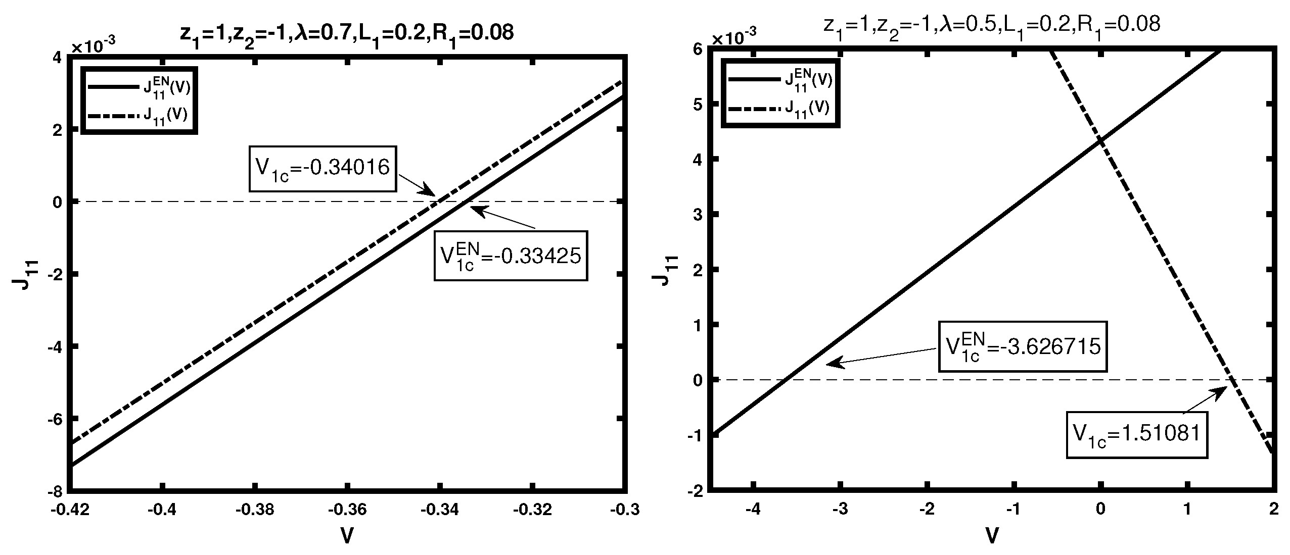
(2)

Identify the critical potentials $V_{1c}$ and $V_{1c}^{EN}$ defined in Definition 1 for different setups in boundary conditions, and observe the monotonicity of $J_1$ and $J_1^{EN}$, respectively, viewed as functions of the potential V, which also indicates the effects on the individual flux $J_1$ from the boundary layers (see Figure 2);

(3)

Identify the critical potentials $V_c$ and $V_c^{EN}$ defined in Definition 1 for different setups in boundary conditions, and observe the monotonicity of $I_1$ and $I_1^{EN}$, respectively, viewed as functions of the potential V, which also indicates the effects on the I–V relations from the boundary layers (see Figure 3).

3.3.2. Direct Description of Boundary Layer Effects on Ionic Flows

To better understand the boundary layer effects on ionic flows, we consider the difference between $J_{k1}^{EN}$ and $J_{k1}$, and the difference between $I_1^{EN}$ and $I_1$. More precisely, we define

$$\begin{array}{cc}\hfill {\mathcal{J}}_{k1}^D=& {\mathcal{J}}_{k1}^D(V;\lambda ,\sigma ,\rho )=J_{k1}(V;\lambda ,\sigma ,\rho )-J_{k1}^{EN}(V,\lambda ,1,1),k=1,2,\hfill \\ \hfill {\mathcal{I}}_1^D=& {\mathcal{I}}_1(V;\lambda ,\sigma ,\rho )=I_1(V;\lambda ,\sigma ,\rho )-I_1^{EN}(V;\lambda ,1,1).\hfill \end{array}$$

From (14), together with ${\beta }_{11}=-{\alpha }_{11}$, one has

$$\begin{array}{cc}\hfill {\mathcal{J}}_{11}^D=& {\alpha }_{10}(\lambda ,\sigma ,\rho )-{\alpha }_{10}(\lambda ,1,1)+({\alpha }_{11}(\lambda ,\sigma ,\rho )-{\alpha }_{11}(\lambda ,1,1))\frac{e}{k_{B}T}V,\hfill \\ \hfill {\mathcal{J}}_{21}^D=& {\beta }_{10}(\lambda ,\sigma ,\rho )-{\beta }_{10}(\lambda ,1,1)-({\alpha }_{11}(\lambda ,\sigma ,\rho )-{\alpha }_{11}(\lambda ,1,1))\frac{e}{k_{B}T}V,\hfill \\ \hfill {\mathcal{I}}_1^D=& z_1{D}_1\left({\alpha }_{10}(\lambda ,\sigma ,\rho )-{\alpha }_{10}(\lambda ,1,1)\right)+z_2{D}_2\left({\beta }_{10}(\lambda ,\sigma ,\rho )-{\beta }_{10}(\lambda ,1,1)\right)\hfill \\ & +(z_1{D}_1-z_2{D}_2)\left({\alpha }_{11}(\lambda ,\sigma ,\rho )-{\alpha }_{11}(\lambda ,1,1)\right)\frac{e}{k_{B}T}V.\hfill \end{array}$$

It follows that (up to the first order in $\sigma$ and $\rho$)

$$\begin{array}{c}\hfill \begin{array}{cc}\hfill \frac{\partial {\mathcal{J}}_{11}^D(V;\lambda ,\sigma ,\rho )}{\partial V}=& -\frac{\partial {\mathcal{J}}_{21}^D(V;\lambda ,\sigma ,\rho )}{\partial V}=\frac{e{R}_1^2}{2k_{B}T{\ln }^{2}x}{\mathcal{A}}_2(x,\sigma ,\rho ),\hfill \\ \hfill \frac{\partial {\mathcal{I}}_1^D(V;\lambda ,\sigma ,\rho )}{\partial V}=& \frac{e{R}_1^2(z_1{D}_1-z_2{D}_2)}{2k_{B}T{\ln }^{2}x}{\mathcal{A}}_2(x,\sigma ,\rho ),\hfill \end{array}\end{array}$$

(25)

where ${\mathcal{A}}_2(x;\sigma ,\rho )$ is given in (18).

Obviously, with ${\mathcal{A}}_2(x;\sigma ,\rho )\ne 0$, the equation ${\mathcal{J}}_{11}^D(V;\lambda ,\sigma ,\rho )=0$ has a unique zero, say $V^{1\ast }$, the equation ${\mathcal{J}}_{21}^D(V;\lambda ,\sigma ,\rho )=0$ has a unique zero, say $V^{2\ast }$, and the equation ${\mathcal{I}}_1^D(V;\lambda ,\sigma ,\rho )=0$ has a unique zero, say $V^{\ast }$. Furthermore, one has

$$\begin{array}{cc}\hfill V^{1\ast }=& -\frac{{\alpha }_{10}(\lambda ,\sigma ,\rho )-{\alpha }_{10}(\lambda ,1,1)}{{\alpha }_{11}(\lambda ,\sigma ,\rho )-{\alpha }_{11}(\lambda ,1,1)}·\frac{k_{B}T}{e},\hfill \\ \hfill V^{2\ast }=& -\frac{{\beta }_{10}(\lambda ,\sigma ,\rho )-{\beta }_{10}(\lambda ,1,1)}{{\beta }_{11}(\lambda ,\sigma ,\rho )-{\beta }_{11}(\lambda ,1,1)}·\frac{k_{B}T}{e},\hfill \\ \hfill V^{\ast }=& -\frac{z_1{D}_1\left({\alpha }_{10}(\lambda ,\sigma ,\rho )-{\alpha }_{10}(\lambda ,1,1)\right)+z_2{D}_2\left({\beta }_{10}(\lambda ,\sigma ,\rho )-{\beta }_{10}(\lambda ,1,1)\right)}{(z_1{D}_1-z_2{D}_2)\left({\alpha }_{11}(\lambda ,\sigma ,\rho )-{\alpha }_{11}(\lambda ,1,1)\right)}.\hfill \end{array}$$

It is not difficult to see that the critical potentials $V^{1\ast }$ (resp. $V^{2\ast }$ and $V^{\ast }$) balance the effects from the boundary layers on the leading term $J_{11}$ (resp. $J_{21}$ and $I_1$) that contains finite ion size effects.

Note that, from (25), the monotonicity of ${\mathcal{J}}_{11}^D(V;\lambda ,\sigma ,\rho ),{\mathcal{J}}_{21}^D(V;\lambda ,\sigma ,\rho )$, and ${\mathcal{I}}_1^D(V;\lambda ,\sigma ,\rho )$ is determined by the sign of ${\mathcal{A}}_2(x;\sigma ,\rho )$, which is discussed in Lemma 4 in detail. For simplicity, here, we assume ${\mathcal{A}}_2\left(x\right)>0$, and establish the following result.

Theorem 6. 

Assuming $L_1>R_1$ and $(\sigma ,\rho )\to (1,1)$. For $\nu >0$ small, one has $\frac{\partial {\mathcal{J}}_{11}^D(V;\lambda ,\sigma ,\rho )}{\partial V}>0$, $\frac{\partial {\mathcal{J}}_{21}^D(V;\lambda ,\sigma ,\rho )}{\partial V}<0$, and $\frac{\partial {\mathcal{I}}_1(V;\lambda ,\sigma ,\rho )}{\partial V}>0$. Moreover,

(i)

$J_1(V;\lambda ,\sigma ,\rho )<J_1^{EN}(V,\lambda ,1,1)$ (resp. $J_1(V;\lambda ,\sigma ,\rho )>J_1^{EN}(V,\lambda ,1,1)$) for $V<V^{1\ast }$ (resp. $V>V^{1\ast }$). In other words, the boundary layers reduce (resp. enhance) the effect on the individual flux $J_1$ from the finite ion size for $V<V^{1\ast }$ (resp. $V>V^{1\ast }$).

(ii)

$J_{21}(V;\lambda ,\sigma ,\rho )>J_{21}^{EN}(V,\lambda ,1,1)$ (resp. $J_2(V;\lambda ,\sigma ,\rho )<J_2^{EN}(V,\lambda ,1,1)$) for $V<V^{2\ast }$ (resp. $V>V^{2\ast }$). In other words, the boundary layers enhance (resp. reduce) the effect on the individual flux $J_2$ from the finite ion size for $V<V^{2\ast }$ (resp. $V>V^{2\ast }$).

(iii)

$I_1(V;\lambda ,\sigma ,\rho )<I_1^{EN}(V,\lambda ,1,1)$ (resp. $I_1(V;\lambda ,\sigma ,\rho )>I_1^{EN}(V,\lambda ,1,1)$) for $V<V^{\ast }$ (resp. $V>V^{\ast }$). In other words, the boundary layers reduce (resp. enhance) the effect on the current I from the finite ion size for $V<V^{\ast }$ (resp. $V>V^{\ast }$).

To end this section, we demonstrate that the boundary layers play crucial roles in the study of ionic flow properties (see Theorems 5 and 6). Particularly, the characterization of the nonlinear interactions between the boundary layer parameters $\sigma$ and $\rho$ and other system parameters (Lemma 4 provides an example) should be considered carefully in the future studies of ion channel problems.

4. Conclusions

In this work, we analyze a quasi-one-dimensional PNP system with finite ion sizes modeled through Bikerman’s local hard-sphere potential. We mainly focus on the effects from boundary layers on ionic flows due to the relaxation of electroneutrality boundary conditions. The detailed analysis provides better understanding of the mechanism of ionic flows through membrane channels. The study is critical because boundary layers of charge are particularly likely to produce artifacts over long distance, which could dramatically affect the behavior of ionic flows. Of particular interest are the leading terms $J_{k1}$ of the individual fluxes and $I_1$ of the I–V relations that contain finite ion size effects. To be specific,

• We study the signs of $J_{k1}$ and $I_1$ with boundary layers, from which one can tell whether the finite ion size enhances or reduces the individual fluxes, $J_k$, and the I–V relation, I.
• We characterize the monotonicity of $J_{k1}$ and $I_1$ with boundary layers about the potential V, from which one can efficiently adjust/control the boundary conditions to enhance or reduce the finite ion size effects.
• We examine the boundary layer effects on ionic flows by considering

  –

  the difference $J_{k1}(V;\sigma ,\rho )-J_{k1}^{EN}(V;1,1)$ and $I_1(V;\sigma ,\rho )-I_1^{EN}(V;1,1)$, where $J_{k1}$ and $I_1$ are with boundary layers, and $J_{k1}^{EN}$ and $I_1^{EN}$ are under electroneutrality boundary conditions;

  –

  the partial orders of the critical potentials $V_{kc},V_c,V_{kc}^{EN}$, and $V_c^{EN}$ described in (22) and (23).

With boundary layers, many nonintuitive phenomena of ionic flows are observed. Among others, we find

• As linear functions of the potential V (fixing other system parameters)

  –

  ${\partial }_V{J}_{11}$ and ${\partial }_V{I}_1$ (resp. ${\partial }_V{J}_{21}$) can be negative (resp. positive), while they are always positive (resp. negative) under the electroneutrality boundary conditions (see Theorems 1 and 3);

  –

  ${\partial }_{V\lambda }{J}_{11}$ and ${\partial }_{V\lambda }{I}_1$ (resp. ${\partial }_{V\lambda }{J}_{21}$) can be negative (resp. positive), while they are always positive (negative) under the electroneutrality boundary conditions (see Theorems 2 and 4).

• Critical potentials that either balance the ion size effects (such as $V_{1c},V_{2c}$, and $V_c$) or separate the relative ion size effects (such as $V^{1c},V^{2c}$, and $V^c$) on individual fluxes, I–V relations, and the total flow rate of matter, respectively, are identified (Definition 1), which play critical roles in studying ionic flow properties of interest and characterizing the effects from boundary layers (discussed in Section 3).

Finally, we demonstrate that the setting of the PNP problem in this work is relatively simple, but our analysis is rigorous. It is an extension of the work performed in [48], and the study provides additional information of the dynamics of ionic flows. This work, together with the work performed in [43,62], could provide some deep insights for future studies of ion channel problems.

References

1. Gillespie, D. A Singular Perturbation Analysis of the Poisson-Nernst-Planck System: Applications to Ionic Channels. Ph.D. Thesis, College of Nursing, Rush University, Chicago, IL, USA, 1999. [Google Scholar]
2. Barcilon, V. Ion flow through narrow membrane channels: Part I. SIAM J. Appl. Math. 1992, 52, 1391–1404. [Google Scholar] [CrossRef]
3. Barcilon, V.; Chen, D.-P.; Eisenberg, R.S. Ion flow through narrow membrane channels: Part II. SIAM J. Appl. Math. 1992, 52, 1405–1425. [Google Scholar] [CrossRef]
4. Eisenberg, R.S. Channels as enzymes. J. Memb. Biol. 1990, 115, 1–12. [Google Scholar] [CrossRef] [PubMed]
5. Eisenberg, R.S. Atomic biology, electrostatics and ionic channels. Adv. Ser. Phys. Chem. Recent Dev. Theor. Stud. Proteins 1996, 7, 269–357. [Google Scholar]
6. Abaid, N.; Eisenberg, R.S.; Liu, W. Asymptotic expansions of I-V relations via a Poisson-Nernst-Planck system. SIAM J. Appl. Dyn. Syst. 2008, 7, 1507–1526. [Google Scholar] [CrossRef]
7. Barcilon, V.; Chen, D.-P.; Eisenberg, R.S.; Jerome, J.W. Qualitative properties of steady-state Poisson-Nernst-Planck systems: Perturbation and simulation study. SIAM J. Appl. Math. 1997, 57, 631–648. [Google Scholar]
8. Chen, D.P.; Eisenberg, R.S. Charges, currents and potentials in ionic channels of one conformation. Biophys. J. 1993, 64, 1405–1421. [Google Scholar] [CrossRef] [PubMed]
9. Eisenberg, B. Proteins, channels, and crowded ions. Biophys. Chem. 2003, 100, 507–517. [Google Scholar] [CrossRef] [PubMed]
10. Gillespie, D.; Eisenberg, R.S. Physical descriptions of experimental selectivity measurements in ion channels. Eur. Biophys. J. 2002, 31, 454–466. [Google Scholar] [CrossRef]
11. Gillespie, D.; Nonner, W.; Eisenberg, R.S. Coupling Poisson-Nernst-Planck and density functional theory to calculate ion flux. J. Phys. Condens. Matter 2002, 14, 12129–12145. [Google Scholar] [CrossRef]
12. Gillespie, D.; Nonner, W.; Eisenberg, R.S. Density functional theory of charged, hard-sphere fluids. Phys. Rev. E 2003, 68, 0313503. [Google Scholar] [CrossRef] [PubMed]
13. Im, W.; Roux, B. Ion permeation and selectivity of OmpF porin: A theoretical study based on molecular dynamics, Brownian dynamics, and continuum electrodiffusion theory. J. Mol. Biol. 2002, 322, 851–869. [Google Scholar] [CrossRef] [PubMed]
14. Roux, B.; Allen, T.W.; Berneche, S.; Im, W. Theoretical and computational models of biological ion channels. Quat. Rev. Biophys. 2004, 37, 15–103. [Google Scholar] [CrossRef]
15. Liu, W.; Wang, B. Poisson-Nernst-Planck systems for narrow tubular-like membrane channels. J. Dyn. Diff. Equ. 2010, 22, 413–437. [Google Scholar] [CrossRef]
16. Nonner, W.; Eisenberg, R.S. Ion permeation and glutamate residues linked by Poisson-Nernst-Planck theory in L-type Calcium channels. Biophys. J. 1998, 75, 1287–1305. [Google Scholar] [CrossRef] [PubMed]
17. Eisenberg, B.; Liu, W. Poisson-Nernst-Planck systems for ion channels with permanent charges. SIAM J. Math. Anal. 2007, 38, 1932–1966. [Google Scholar] [CrossRef]
18. Bates, P.W.; Wen, Z.; Zhang, M. Small permanent charge effects on individual fluxes via Poisson-Nernst-Planck models with multiple cations. J. Nonlinear Sci. 2021, 31, 62. [Google Scholar] [CrossRef]
19. Burger, M.; Eisenberg, R.S.; Engl, H.W. Inverse problems related to ion channel selectivity. SIAM J. Appl. Math. 2007, 67, 960–989. [Google Scholar] [CrossRef]
20. Cardenas, A.E.; Coalson, R.D.; Kurnikova, M.G. Three-Dimensional Poisson-Nernst-Planck Theory Studies: Influence of Membrane Electrostatics on Gramicidin A Channel Conductance. Biophys. J. 2000, 79, 80–93. [Google Scholar] [CrossRef]
21. Chen, J.; Zhang, M. Geometric singular perturbation approach to Poisson-Nernst-Planck systems with local hard-sphere potential: Studies on zero-current ionic flows with boundary layers. Qual. Theory Dyn. Syst. 2022, 21, 139. [Google Scholar] [CrossRef]
22. Coalson, R.; Kurnikova, M. Poisson-Nernst-Planck theory approach to the calculation of current through biological ion channels. IEEE Trans. Nanobiosci. 2005, 4, 81–93. [Google Scholar] [CrossRef]
23. Graf, P.; Kurnikova, M.G.; Coalson, R.D.; Nitzan, A. Comparison of Dynamic Lattice Monte-Carlo Simulations and Dielectric Self Energy Poisson-Nernst-Planck Continuum Theory for Model Ion Channels. J. Phys. Chem. B 2004, 108, 2006–2015. [Google Scholar] [CrossRef]
24. Hollerbach, U.; Chen, D.-P.; Eisenberg, R.S. Two- and Three-Dimensional Poisson-Nernst-Planck Simulations of Current Flow through Gramicidin-A. J. Comp. Sci. 2002, 16, 373–409. [Google Scholar] [CrossRef]
25. Hollerbach, U.; Chen, D.; Nonner, W.; Eisenberg, B. Three-dimensional Poisson-Nernst-Planck Theory of Open Channels. Biophys. J. 1999, 76, A205. [Google Scholar]
26. Hyon, Y.; Fonseca, J.; Eisenberg, B.; Liu, C. A new Poisson-Nernst-Planck equation (PNP-FS-IF) for charge inversion near walls. Biophys. J. 2011, 100, 578a. [Google Scholar] [CrossRef]
27. Jerome, J.W. Mathematical Theory and Approximation of Semiconductor Models; Springer: New York, NY, USA, 1995. [Google Scholar]
28. Jerome, J.W.; Kerkhoven, T. A finite element approximation theory for the drift-diffusion semiconductor model. SIAM J. Numer. Anal. 1991, 28, 403–422. [Google Scholar] [CrossRef]
29. Ji, S.; Eisenberg, B.; Liu, W. Flux ratios and channel structures. J. Dyn. Diff. Equ. 2019, 31, 1141–1183. [Google Scholar] [CrossRef]
30. Kurnikova, M.G.; Coalson, R.D.; Graf, P.; Nitzan, A. A Lattice Relaxation Algorithm for 3D Poisson-Nernst-Planck Theory with Application to Ion Transport Through the Gramicidin A Channel. Biophys. J. 1999, 76, 642–656. [Google Scholar] [CrossRef]
31. Liu, W.; Sun, N. Flux ratios for effects of permanent charges on ionic flows with three ion species: New phenomena from a case study. J. Dyn. Diff. Equ. 2004, 26, 27–62. [Google Scholar] [CrossRef]
32. Liu, W.; Xu, H. A complete analysis of a classical Poisson-Nernst-Planck model for ionic flow. J. Diff. Equ. 2015, 258, 1192–1228. [Google Scholar] [CrossRef]
33. Liu, C.; Wang, C.; Wise, S.; Yue, X.; Zhou, S. A positivity preserving, energy stable and convergent numerical scheme for the Poisson-Nernst-Planck system. Math. Comput. 2021, 90, 2071–2106. [Google Scholar] [CrossRef]
34. Park, J.-K.; Jerome, J.W. Qualitative properties of steady-state Poisson-Nernst-Planck systems: Mathematical study. SIAM J. Appl. Math. 1997, 57, 609–630. [Google Scholar] [CrossRef]
35. Rubinstein, I. Multiple steady states in one-dimensional electrodiffusion with local electroneutrality. SIAM J. Appl. Math. 1987, 47, 1076–1093. [Google Scholar] [CrossRef]
36. Rubinstein, I. Electro-Diffusion of Ions. In SIAM Studies in Applied Mathematics; SIAM: Philadelphia, PA, USA, 1990. [Google Scholar]
37. Singer, A.; Norbury, J. A Poisson-Nernst-Planck model for biological ion channels–an asymptotic analysis in a three-dimensional narrow funnel. SIAM J. Appl. Math. 2009, 70, 949–968. [Google Scholar] [CrossRef]
38. Singer, A.; Gillespie, D.; Norbury, J.; Eisenberg, R.S. Singular perturbation analysis of the steady-state Poisson-Nernst-Planck system: Applications to ion channels. Eur. J. Appl. Math. 2008, 19, 541–560. [Google Scholar] [CrossRef] [PubMed]
39. Steinrück, H. Asymptotic analysis of the current-voltage curve of a pnpn semiconductor device. IMA J. Appl. Math. 1989, 43, 243–259. [Google Scholar] [CrossRef]
40. Steinrück, H. A bifurcation analysis of the one-dimensional steady-state semiconductor device equations. SIAM J. Appl. Math. 1989, 49, 1102–1121. [Google Scholar] [CrossRef]
41. Wang, X.-S.; He, D.; Wylie, J.; Huang, H. Singular perturbation solutions of steady-state Poisson-Nernst-Planck systems. Phys. Rev. E 2014, 89, 022722. [Google Scholar] [CrossRef] [PubMed]
42. Wen, Z.; Bates, P.W.; Zhang, M. Effects on I-V relations from small permanent charge and channel geometry via classical Poisson-Nernst-Planck equations with multiple cations. Nonlinearity 2021, 34, 4464–4502. [Google Scholar] [CrossRef]
43. Wen, Z.; Zhang, L.; Zhang, M. Dynamics of classical Poisson-Nernst-Planck systems with multiple cations and boundary layers. J. Dyn. Diff. Equ. 2021, 33, 211–234. [Google Scholar] [CrossRef]
44. Zhang, M. Boundary layer effects on ionic flows via classical Poisson-Nernst-Planck systems. Comput. Math. Biophys. 2018, 6, 14–27. [Google Scholar] [CrossRef]
45. Zheng, Q.; Chen, D.; Wei, W. Second-order Poisson-Nernst-Planck solver for ion transport. J. Comput. Phys. 2011, 230, 5239–5262. [Google Scholar] [CrossRef] [PubMed]
46. Zheng, Q.; Wei, G.W. Poisson-Boltzmann-Nernst-Planck model. J. Chem. Phys. 2011, 134, 1–17. [Google Scholar] [CrossRef] [PubMed]
47. Zhang, L.; Liu, W. Effects of large permanent charges on ionic flows via Poisson-Nernst-Planck models. SIAM J. Appl. Dyn. Syst. 2020, 19, 1993–2029. [Google Scholar] [CrossRef]
48. Jia, Y.; Liu, W.; Zhang, M. Qualitative properties of ionic flows via Poisson-Nernst-Planck systems with Bikerman’s local hard-sphere potential: Ion size effects. Discret. Contin. Dyn. Syst. Ser. B 2016, 21, 1775–1802. [Google Scholar] [CrossRef]
49. Ding, J.; Wang, Z.; Zhou, S. Positivity preserving finite difference methods for Poisson-Nernst-Planck equations with steric interactions: Application to slit-shaped nanopore conductance. J. Comput. Phys. 2019, 397, 108864. [Google Scholar] [CrossRef]
50. Eisenberg, B.; Hyon, Y.; Liu, C. Energy variational analysis of ions in water and channels: Field theory for primitive models of complex ionic fluids. J. Chem. Phys. 2010, 133, 104104. [Google Scholar] [CrossRef] [PubMed]
51. Hyon, Y.; Eisenberg, B.; Liu, C. A mathematical model for the hard sphere repulsion in ionic solutions. Commun. Math. Sci. 2011, 9, 459–475. [Google Scholar]
52. Hyon, Y.; Liu, C.; Eisenberg, B. PNP equations with steric effects: A model of ion flow through channels. J. Phys. Chem. B 2012, 116, 11422–11441. [Google Scholar]
53. Kilic, M.S.; Bazant, M.Z.; Ajdari, A. Steric effects in the dynamics of electrolytes at large applied voltages. II. Modified Poisson-Nernst-Planck equations. Phys. Rev. E 2007, 75, 021503. [Google Scholar] [CrossRef]
54. Sun, L.; Liu, W. Non-localness of excess potentials and boundary value problems of Poisson-Nernst-Planck systems for ionic flow: A case study. J. Dyn. Diff. Equ. 2018, 30, 779–797. [Google Scholar] [CrossRef]
55. Zhou, S.; Wang, Z.; Li, B. Mean-field description of ionic size effects with nonuniform ionic sizes: A numerical approach. Phy. Rev. E 2011, 84, 1–13. [Google Scholar] [CrossRef] [PubMed]
56. Bikerman, J.J. Structure and capacity of the electrical double layer. Philos. Mag. 1942, 33, 384. [Google Scholar] [CrossRef]
57. Eisenberg, B.; Liu, W.; Xu, H. Reversal charge and reversal potential: Case studies via classical Poisson-Nernst-Planck models. Nonlinearity 2015, 28, 103–127. [Google Scholar] [CrossRef]
58. Ji, S.; Liu, W. Poisson-Nernst-Planck systems for ion flow with density functional theory for hard-sphere potential: I–V relations and critical potentials. Part I: Analysis. J. Dyn. Diff. Equ. 2012, 24, 955–983. [Google Scholar] [CrossRef]
59. Liu, W. Geometric singular perturbation approach to steady-state Poisson-Nernst-Planck systems. SIAM J. Appl. Math. 2005, 65, 754–766. [Google Scholar] [CrossRef]
60. Liu, W. One-dimensional steady-state Poisson-Nernst-Planck systems for ion channels with multiple ion species. J. Diff. Equ. 2009, 246, 428–451. [Google Scholar] [CrossRef]
61. Aitbayev, R.; Bates, P.W.; Lu, H.; Zhang, L.; Zhang, M. Mathematical studies of Poisson-Nernst-Planck systems: Dynamics of ionic flows without electroneutrality conditions. J. Comput. Appl. Math. 2019, 362, 510–527. [Google Scholar] [CrossRef]
62. Chen, J.; Wang, Y.; Zhang, L.; Zhang, M. Mathematical analysis of Poisson-Nernst-Planck models with permanent charges and boundary layers: Studies on individual fluxes. Nonlinearity 2021, 34, 3879–3906. [Google Scholar] [CrossRef]
63. Lu, H.; Li, J.; Shackelford, J.; Vorenberg, J.; Zhang, M. Ion size effects on individual fluxes via Poisson-Nernst-Planck systems with Bikerman’s local hard-sphere potential: Analysis without electroneutrality boundary conditions. Discret. Contin. Dyn. Syst. Ser. B 2018, 23, 1623–1643. [Google Scholar] [CrossRef]
64. Wang, Y.; Zhang, L.; Zhang, M. Studies on individual fluxes via Poisson-Nernst-Planck models with small permanent charges and partial electroneutrality conditions. J. Appl. Anal. Comput. 2022, 12, 87–105. [Google Scholar] [CrossRef] [PubMed]
Figure 1. Graph of function F ( x ) . The left graph corresponds to statement (ii1) of Lemma 5, while the right one corresponds to statement (ii2).
Mathematics 12 01182 g001
Figure 2. The left figure is a graph of J 11 ( V ) with σ = 1.001 and ρ = 1.002 (dashed line), and J 11 E N ( V ) with σ = ρ = 1 (solid line) for x > x , while the right one is 1 < x < x . The left figure shows that both J 11 and J 11 E N have the same monotonicity, while the right one shows opposite monotonicity.
Mathematics 12 01182 g002
Figure 3. The left figure is a graph of I 11 ( V ) with σ = 1.001 and ρ = 1.002 (dashed line), and I 11 E N ( V ) with σ = ρ = 1 (solid line) for x > x , while the right one is 1 < x < x . The left figure shows that both I 1 and I 1 E N have the same monotonicity, while the right one shows opposite monotonicity.
Mathematics 12 01182 g003
Disclaimer/Publisher’s Note: The statements, opinions and data contained in all publications are solely those of the individual author(s) and contributor(s) and not of MDPI and/or the editor(s). MDPI and/or the editor(s) disclaim responsibility for any injury to people or property resulting from any ideas, methods, instructions or products referred to in the content.