Abstract
Recently, a mixed redundancy was introduced among the redundant design strategies to achieve a more reliable system within the equivalent resources. This study deals with a lifetime distribution for a mixed redundant system with an imperfect fault detector/switch. The lifetime distribution model was formulated using a structured continuous Markov chain (CTMC) and considers the time-to-failure (TTF) distribution of a component as a phase-type distribution (PHD). The model’s versatility and practicality are enhanced because the PHD can represent diverse degradation patterns of the components exposed to varied operating environments. The model provides accurate reliability for a mixed redundant system by advancing the approximate reliability function suggested in previous studies. Furthermore, the model would be useful in system design and management because it provides information such as the nth moment of the system’s lifetime distribution. In numerical experiments on some examples, the mixed redundancy was confirmed to devise a more reliable system than the existing active and standby redundancies, and the improvement effect increased as the number of redundant components decreased. The optimal structure for maximizing the expected lifetime of the system changes depends on the reliability of the components and fault detector/switch.
Keywords:
system lifetime; reliability design; mixed redundancy; structured Markov chain; phase–type distribution MSC:
90B25
1. Introduction
Traditionally, redundant designs, such as active and standby structures, have been considered to enhance system reliability. In an active redundant system, all the components start operating simultaneously and are exposed to the same operating stress. In addition, the longevity of the system depends on the longest lifetime of the component. A system with standby redundancy consists of both primary components and spares. The primary components start functioning when the system is turned on, and the reserves are activated sequentially when the functional part fails. Thus, the system requires a supplementary apparatus, called a fault detector/switch (abbreviated as a switch), to detect the failure of the operating component and transfer its function to one of the spare components on standby. Assuming that the switch is a fault-free device, a standby redundancy strategy is preferred over an active redundancy for system reliability [1,2]. However, considering that the switch is imperfect, that is, switch reliability is less than 1.0, Coit [3] showed that the optimal redundancy strategy should be employed depending on the condition of the redundant design, such as the reliability and redundancy level of the switch and components. Since then, many studies, such as [3,4,5,6,7,8,9,10,11,12,13], have presented the reliability optimization problem of employing either an active or cold standby (hereafter referred to as standby) redundancy strategy for each subsystem. Moreover, the reliability optimization problem has been applied in various real-world industrial fields such as spaceflight [14], manufacturing systems [15], and sliding window systems [16].
New versions of the optimization problems for system reliability design, such as a redundancy allocation problem (RAP) and a reliability–redundancy allocation problem (RRAP), have been proposed using the reliability function for the mixed redundant system suggested in [17]. When several alternative components for each subsystem perform the identical function but have different features, a RAP simultaneously determines components, redundancy levels, and strategies for the subsystems to maximize system reliability. Thus, the RAP would be generally applied to create a system with components already developed for each subsystem. An RRAP is an integrated form of the reliability allocation problem and the RAP, and it determines the components’ reliability, redundancy levels, and strategies for individual subsystems. Determining the component’s reliability means the component should be newly researched and developed for a subsystem. Ardakan and Hamadani [17] have also proposed a RAP with either an active, standby or mixed redundancy strategy for each subsystem and showed that the mixed redundancy strategy could achieve higher system reliability than other strategies based on the numerical experiments on well-known benchmarks. The best system structures presented in [17,18] have been searched by a genetic algorithm (GA) [19,20] that does not guarantee the optimal solution. Thus, to intactly review the reliability improvement effect of the mixed redundancy strategy, Sadeghi and Roghanian [21] have exploited the optimal solutions obtained by a general algebraic modeling system (GAMS) for the same RAP. Some studies, such as [22,23,24,25,26,27], have extended RAP to allow for subsystems composed of heterogeneous components. In refs. [24,28,29,30,31], new RRAP formulations have been suggested for a system consisting of subsystems that apply a mixed redundancy strategy with heterogeneous components. However, because most of the abovementioned studies are based on the lower bound of mixed redundant system reliability, the effect of improving system reliability by mixed redundancy analyzed in previous studies includes some errors. Although the error may be numerically small, it would be sufficiently meaningful in systems requiring high reliability, such as satellites, aircraft, medical and safety equipment.
To measure the exact reliability of a system using a mixed redundancy strategy, Guilani et al. [31,32] and Peiravi et al. [33] suggested a continuous-time Markov chain (CTMC) model that describes the operating mechanism of the system. In addition, Peiravi et al. [33] reported that the CTMC model significantly improves system reliability and computational time in numerical experimentations based on the same benchmark RAP compared with the approximated reliability function. However, the models are applicable only if the components have a constant hazard function because the proposed CTMC models [31,32,33] assume that a component’s time-to-failure (TTF) is exponentially distributed. To create a new reliability model, the researchers have attempted to obtain a more generalized TTF distribution to represent diverse degradation patterns of components exposed to varied operating environments, such as loading, friction, thermal fatigue, vibration, and chemical and electrical stresses [34]. Therefore, to formulate the lifetime distribution of a mixed redundant system with an imperfect switch, this study suggests a new CTMC model and the TTFs of the system components are distributed according to the generalized phase–type distribution (PHD). The PHD can describe any random distribution well and can represent all the distributions with finite support on non-negative integers [35]. The lifetime distribution model provides accurate system reliability and contains valuable information on the system lifetime, such as the expectation and variance. Based on the optimal reliability of a system in the well-known benchmark for the RAP that has been used in the existing studies, the reliability improvement effect of the mixed redundancy strategy compared to other strategies, such as active and standby redundancies, and the approximation error of the previous reliability function for a mixed redundant system were analyzed. The benchmark considers that the TTFs of the components are distributed according to , which is a specific form of the PHD, and has upper bounds on the cost () and weight () of the system.
The remainder of this paper is organized as follows. Section 2 reviews the reliability model for a system with mixed redundancy proposed by Ardakan and Hamadani [17]. Section 3 proposes a new reliability model for a mixed redundant system with imperfect switching and components with phase–type TTF distributions. Based on the numerical experiments and the optimal solutions of the well-known benchmark problems for the RAP, Section 4 reviews the characteristics of the mixed redundancy strategy, the approximation error of the previous reliability model [17], and the effectiveness of improving the system reliability by considering the mixed redundancy strategy. Finally, Section 5 presents the conclusions and topics for future research.
2. Review on Previous Reliability Model
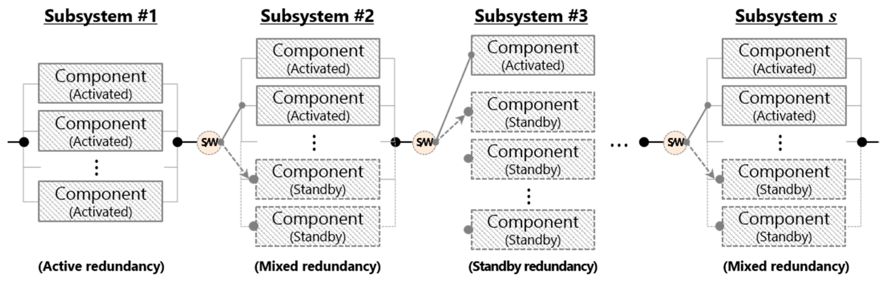
Ardakan and Hamadani [17] first proposed a mixed redundancy strategy in which some components could be applied by active redundancy, whereas others are employed by standby redundancy when the system starts up, as shown in Figure 1. In other words, when a failure is detected in all the activating components, redundant standby components are sequentially hired to maintain the system’s functionality. Table 1 is adapted from [17] and describes the strategies for the redundant design based on the number of active () and standby () redundant components.
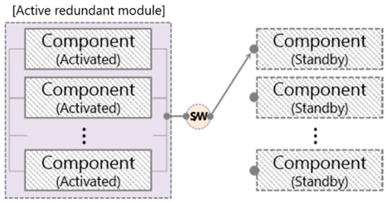
Figure 1.
A system with mixed redundancy.

Table 1.
Strategies for the redundant design.
Ardakan and Hamadani [17] presented Equation (1) as a reliability function for a mixed redundancy system. As mentioned by Coit [36], it is complicated to implement in a closed form using Equation (1); therefore, they proposed Equation (2) to handily compute the lower bound, , of the system reliability. In Equation (2), the reliability of a switch at mission time , always has a smaller value than because . Thus, it could be instinctively discovered that the approximation error, , grows when mission times are long over, or the switch’s reliability decreases. Moreover, Sadeghi and Roghanian [21] and Kim and Kim [34] analyzed the error caused by the above approximation method through numerical experiments as follows:
where is the reliability of the module with active redundancy with components; thus, . is the probability density function (PDF) for the maximum TTF () of the active redundant module. Symbolically, and . Let be the PDF for the component TTF; then, is the PDF for the sum of components’ TTF, that is, it is the -fold convolution of .
3. Proposed Reliability Model
3.1. TTF Distribution of a Component
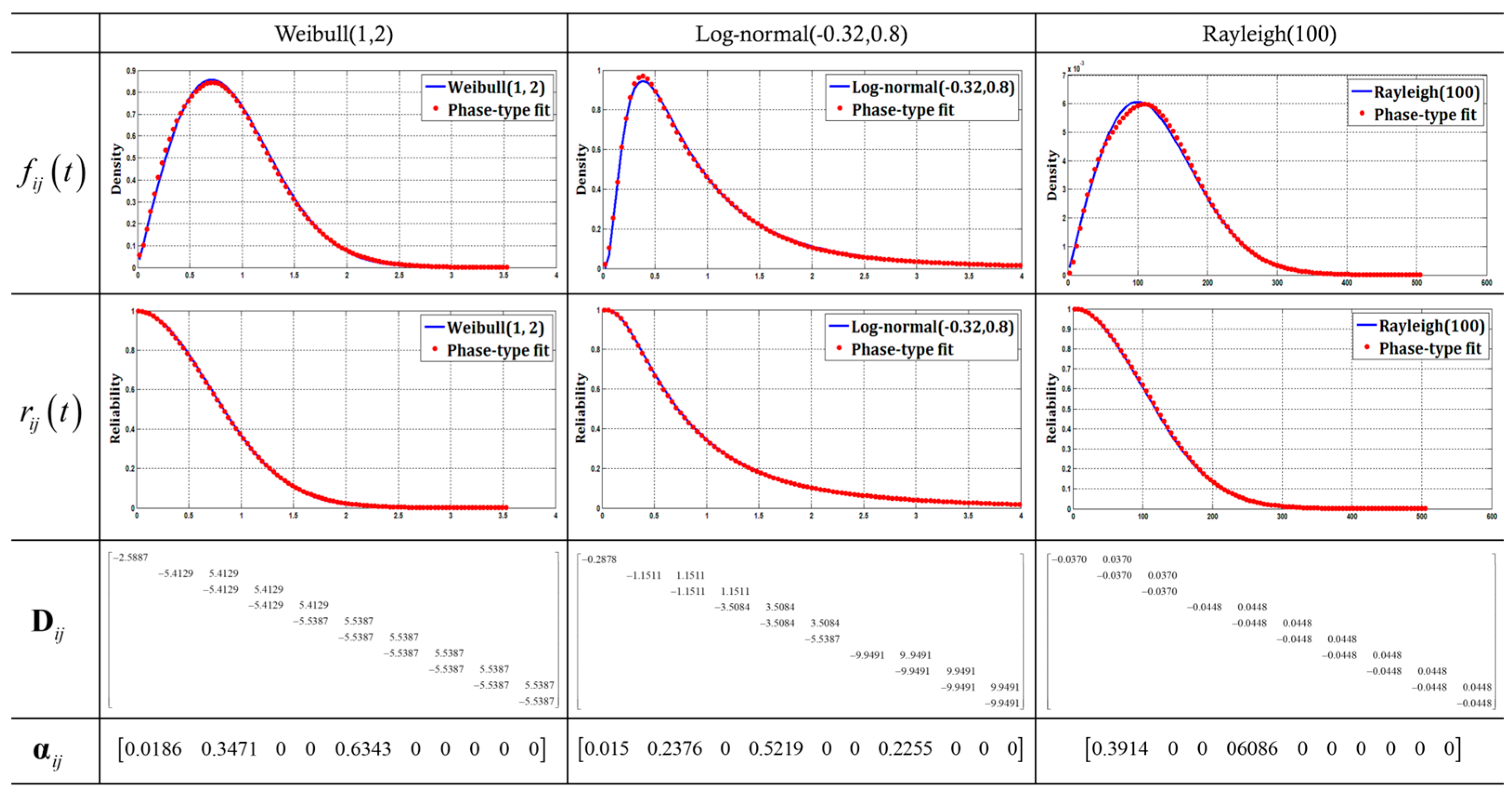
Kim and Kim [34] proposed a PHD to model the generalized component TTF. As shown in Figure 2, the PHD is a probability distribution constructed by a convolution or a mixture of exponential distributions and involves all exponential family distributions, such as exponential, hyper-/hypo-exponential, Erlang, Gamma, and hyper-Erlang distributions. Furthermore, it has considerable flexibility and practicality in system lifetime analysis, such as system reliability, expectation, and the variance of the system lifetime because it can describe any random distribution well and can represent all the distributions with finite support on non-negative integers [35]. Figure 3 is adapted from [34] and shows instances of approximations to the general distribution of the PHD. It includes the initial probability vector and transition rate matrix (TRM) between the transient states.
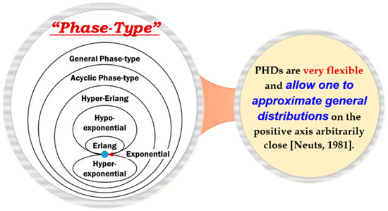
Figure 2.
The flexibility and practicality of PHDs [35].
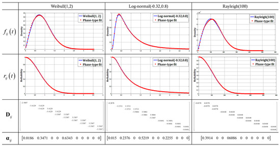
Figure 3.
Instances of the PHDs describing general distributions.
3.2. Reliability of a Component
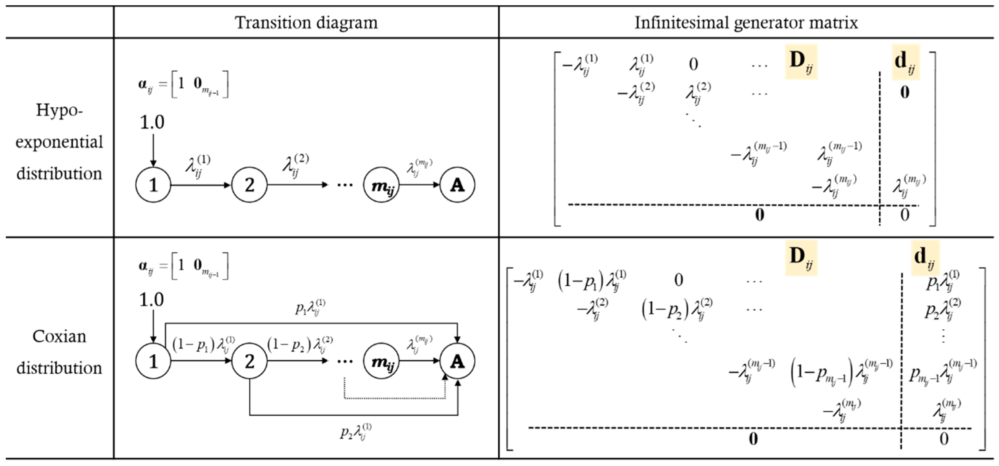
This study considers that the TTFs of the components are distributed according to the generalized PHDs. The PHD consists of transient states () and an absorbing state (), and it is defined as the time required to reach an absorbing state. The transient states describe the degradation of the component during operation, and the absorbing state indicates the failure of the component. Thus, a component normally operates while it remains in the transient state and is broken at the moment of transition to the absorbing state. The PHD for the component of system is represented as , where is a row vector of size denoting the initial probabilities of a CTMC and is a TRM of size to describe the transitions among the transient states in the CTMC. The infinitesimal generator for , which includes the absorbing state, is given by Equation (3) as follows:
where, is the intensity vector of size describing the transitions from the transient states to the absorption, and denotes a row vector of zeros of length . Thus, the dimension of is equal to . For example, Figure 4 shows the infinitesimal generators and the transition mechanism in the components with hypo-exponential (or generalized Erlang) and Coxian TTF distributions, which are specific forms of generalized PHDs.

Figure 4.
Examples of state transition mechanism.
Finally, the reliability function for a component with an infinitesimal generator, as in Equation (3), is presented in Equation (4) as follows:
where denotes the matrix exponential; denotes a column vector of ones of length , which is used for summing the probabilities of the transient states.
3.3. Reliability of Active Redundant Module
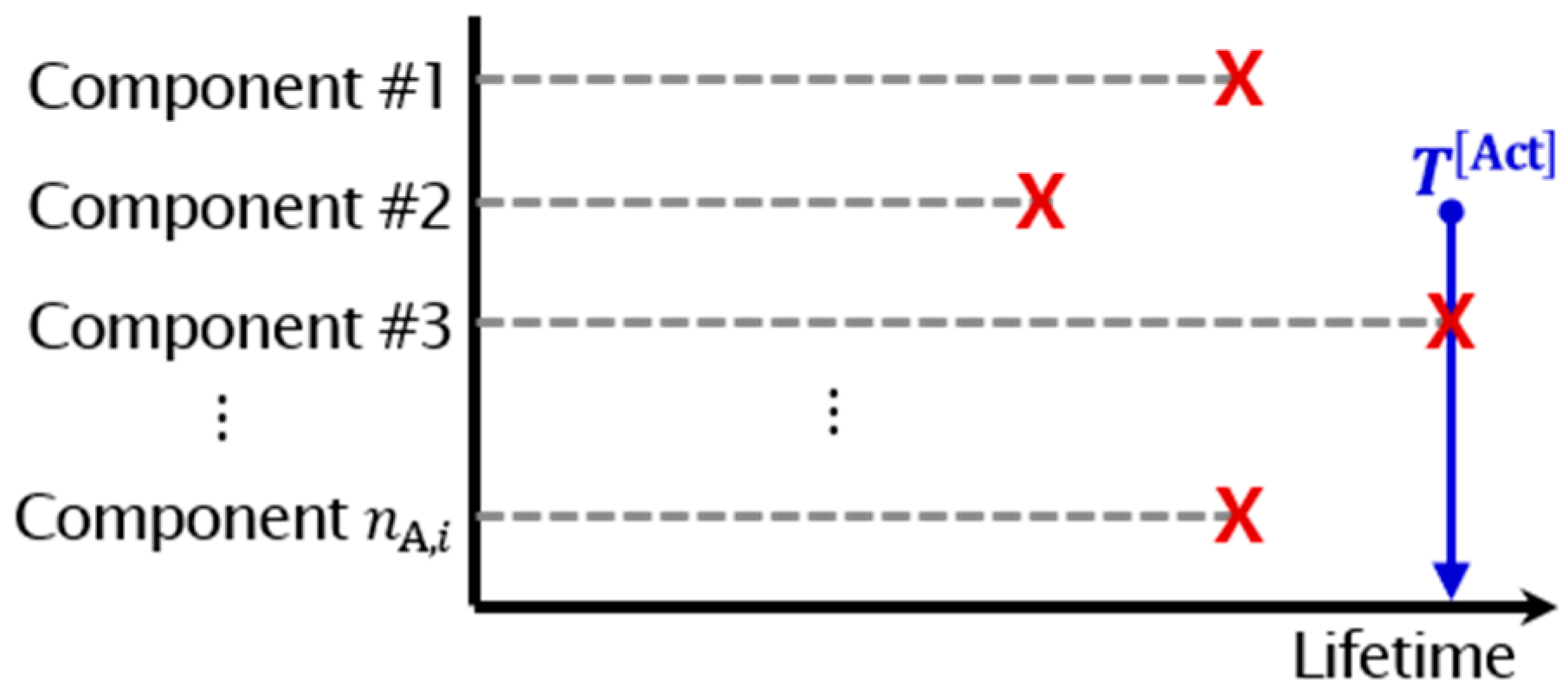
In an active redundant module, all the components are concurrently activated when the system starts operating. The reliability function for the module with components can be presented as . However, in this study, the module is considered as one of the components of a mixed redundant system. To integrate the TTFs of the standby redundant components of the system, a TRM expressing its TTF is required. As shown in Figure 5, the lifetime, , of the module is determined by the longest lifetime of components, symbolically, .

Figure 5.
Lifetime of an active redundant module.
It implies that the active redundant module malfunctions when the states of all the components reach their individual absorption. Thus, the infinitesimal generator, , for the lifetime, , of the module should cover all the combinations of the transient states and the absorbing state for the infinitesimal generators of the components. According to Buchholz [37], for of the active redundant module, the infinitesimal generator, , and the initial probability vector, , are generated as presented in Equation (5):
where, is a dummy variable; thus, and mean that the Kronecker product and sum operations are repeated n times, respectively. Considering for components’ TTF as a square matrix of size , is a row vector of length , and is a square matrix of size . , a submatrix of , is a square matrix of size and describes transient states for the module. is the column vector of size and expresses the global absorbing state in which all the components have reached the absorbing state.
3.4. Reliability of a Mixed Redundant System
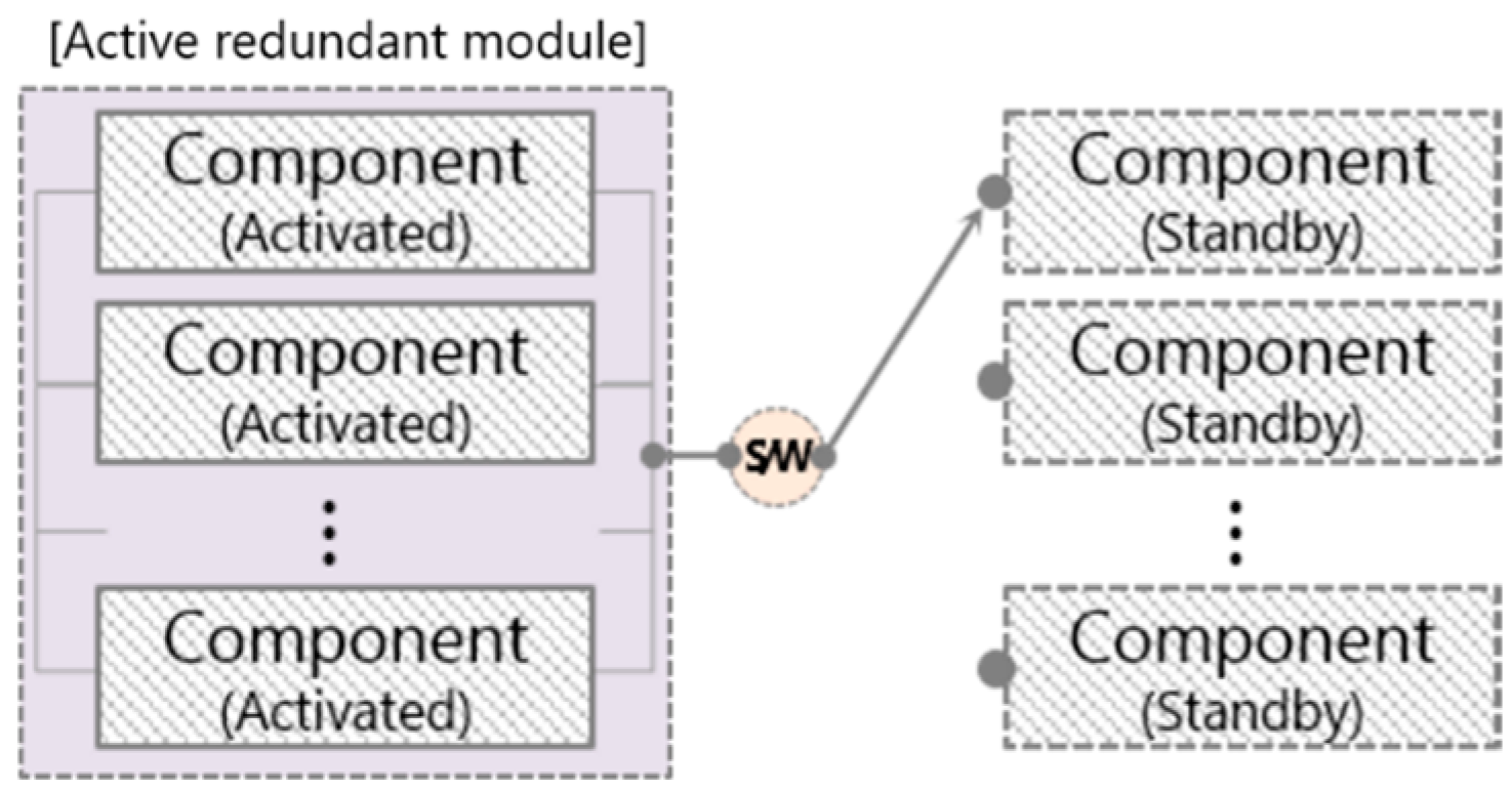
Mixed redundant system consists of an active redundant module (), standby components (), and a fault detector/switch (hereafter referred to as switch) to detect the failure in the activating components and transfer the function to another component. The system assumes that the components on standby do not deteriorate because they are completely protected against the operational stresses, and the failure of a switch implies that the function of activating components cannot be switched over to a standby state. For an imperfect switch, the initial probability vector is denoted as , and the infinitesimal generator, , is represented by Equation (6) as follows:
The integration process between the TRM, , of the active redundant module and TRMs, , of the standby redundant components follows the procedure presented by Kim and Kim [34]. Based on whether the switch operates, they are divided into two situations, and TRMs describing the operating mechanism of the system in each situation have been developed and adequately integrated.
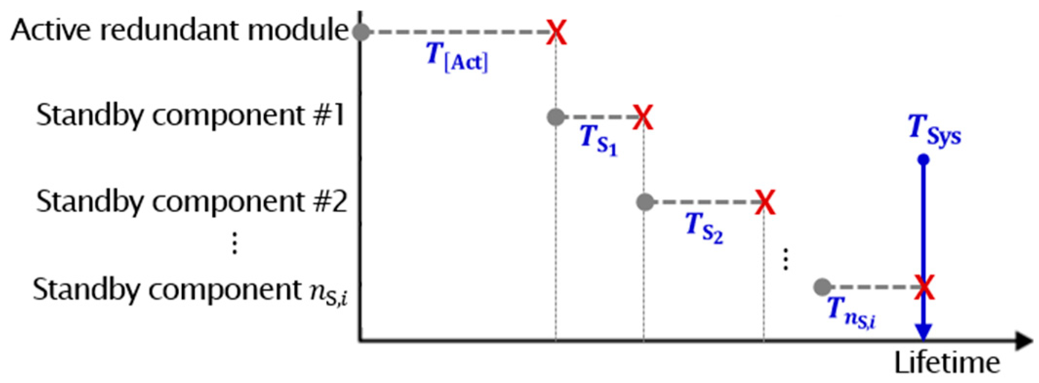
[Situation#1(S1)] In the switch-on condition, the system operates until the last standby component fails because the switchover of an assigned function between the components can be performed in sequence. In other words, if all components of the active redundant module fail, the first standby redundancy component is activated. Also, if the activated component fails, the mission is transferred to the next standby component. Thus, as shown in Figure 6, the system lifetime, , is defined as the sum of the lifetime of the active redundant module and the lifetimes of the standby redundant components; symbolically, . The initial probability vector () and infinitesimal generator () for are expressed by Equations (7) and (8), respectively:
where and denote the initial probabilities that the operation of the active redundant module and standby components start from the absorbing state , i.e., failure, respectively. In general, they could be assumed to be zero; thus, and are row vectors of zeros of size as follows:
where is the sub-TRM for entering the initial state of the first standby component when the active redundant module fails. Similarly, is the sub-TRM activating the standby component when the standby component fails.
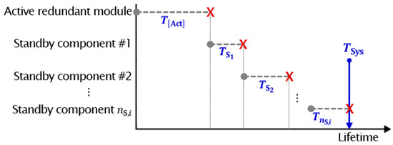
Figure 6.
System lifetime when fault detector/switch operates.
[Situation#2(S2)] In switch-off condition, the failure of an activating component causes system failure because the switch cannot detect the failure and switch the function to another standby, as shown in Figure 7. Thus, the initial probability vector and infinitesimal generator for the are expressed by Equations (9) and (10), respectively:
where depicts the degradation of the standby component, while indicates that the failure of the standby component causes system failure.
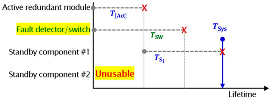
Figure 7.
System lifetime when fault detector/switch fails.
To integrate the above TRMs, and , according to the operating mechanism of a mixed redundant system, the transition probability matrices (TPMs), as in Equation (11), are employed. For Situation#1(S1), conserves the components’ states when the state transition of a switch transpires. For Situation#2(S2), indicates that the state transition turns up in only an activated component when the switch has already broken. The relationship between two TPMs is expressed as .
The initial probability vector, , for the mixed redundant system is presented in Equation (12). When the system remains functional, the sub-TRM , which describes the state transitions of the active redundant module and standby components, is formulated as in Equation (13) [34]:
where is the probability that the switch fails when the system starts; thus, it could be assumed to be zero, generally. Finally, is the row vector of the zeros of length :
where, describes the transitions between the combinatorial states of components’ transient states in the system when the switch is normally operating [Situation#1(S1)]. depicts the state transition of components when the switch has failed [Situation#2(S2)].
Finally, for the lifetime distribution of a mixed redundant system , the reliability, , and hazard function, , at time and the moment, , are presented as Equations (14)–(16), respectively. When in Equation (16), the expected lifetime, , of the system, i.e., mean time-to-failure (MTTF), is suggested as Equation (17). Moreover, Equation (16) provides various information on the system lifetime, such as variance, skewness, and kurtosis. The information would be utilized for system design and management.
4. Numerical Experiments
In this section, the characteristics of the mixed redundancy strategy are reviewed through general numerical experiments considering system design factors such as the reliabilities of components and a switch, the number of redundant components, and the mission time. In addition, based on the well-known benchmark for an RAP, the approximation error of the previous reliability model [17] for a mixed redundant system and the effectiveness of improving the system reliability by considering the mixed redundancy strategy are examined.
4.1. Characteristics of the Mixed Redundancy Strategy
Numerical experiments for reviewing the characteristics of the mixed redundancy strategy assume that the TTFs of components and a switch are distributed according to , that is, an exponential distribution. Since, the active redundancy strategy is always preferred over standby and mixed redundancies when the switch reliability, , is less than the reliability, , of the components; this study reviews the characteristics in a condition where for all [3,36].
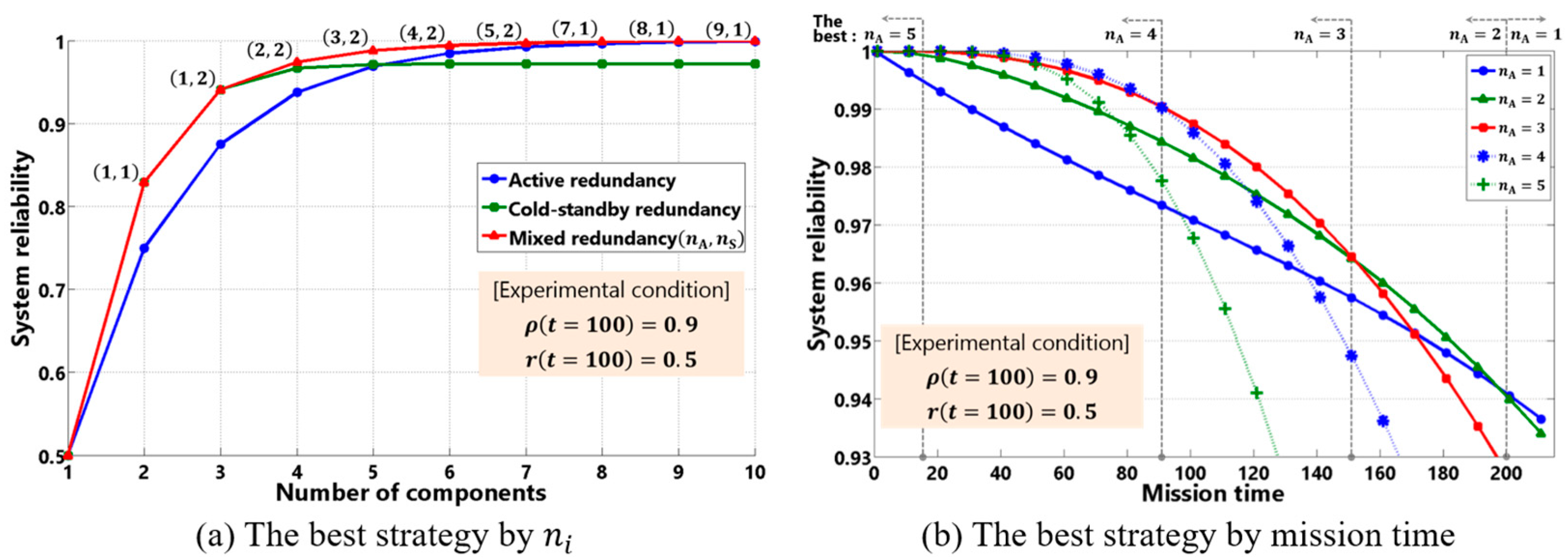
Figure 8a is created assuming that and , when the mission time is given as 100 h. As the number of components () increases, the reliabilities of the active redundant system () and mixed redundant system (, ) are observed to approach 1.0; however, the reliability of the standby redundant system () converges to about 0.9717 from when . Moreover, although the gap between the reliabilities of the active and mixed redundant systems decreases with the increasing number of components, the mixed redundant system always has the highest reliability. In particular, in the practical situation of installing fewer redundant components, there is a significant difference between the reliability of the active and mixed redundancy strategies. In conclusion, the benefit of a mixed redundancy strategy over an active redundancy increases as the number of redundant components decreases.

Figure 8.
Review the best redundancy strategy based on system reliability.
In the design process of reliability, the general aim is to search for the optimal configuration to maximize the system’s reliability at a predetermined mission time. Based on a system with an imperfect switch and five components , Figure 8b observes the change in the reliability of the five configurations over the system’s operating time. The best configuration achieving the highest reliability by the time interval is the following: (5, 0) on the time interval , (4, 1) on the time interval , (3, 2) the time interval , (2, 3) on the time interval , and (1, 4) after 197 h. Therefore, when attempting to maximize system reliability at a predetermined mission time by installing the same number of components, increasing the number of standby redundant components may be recommended as the mission time expands.
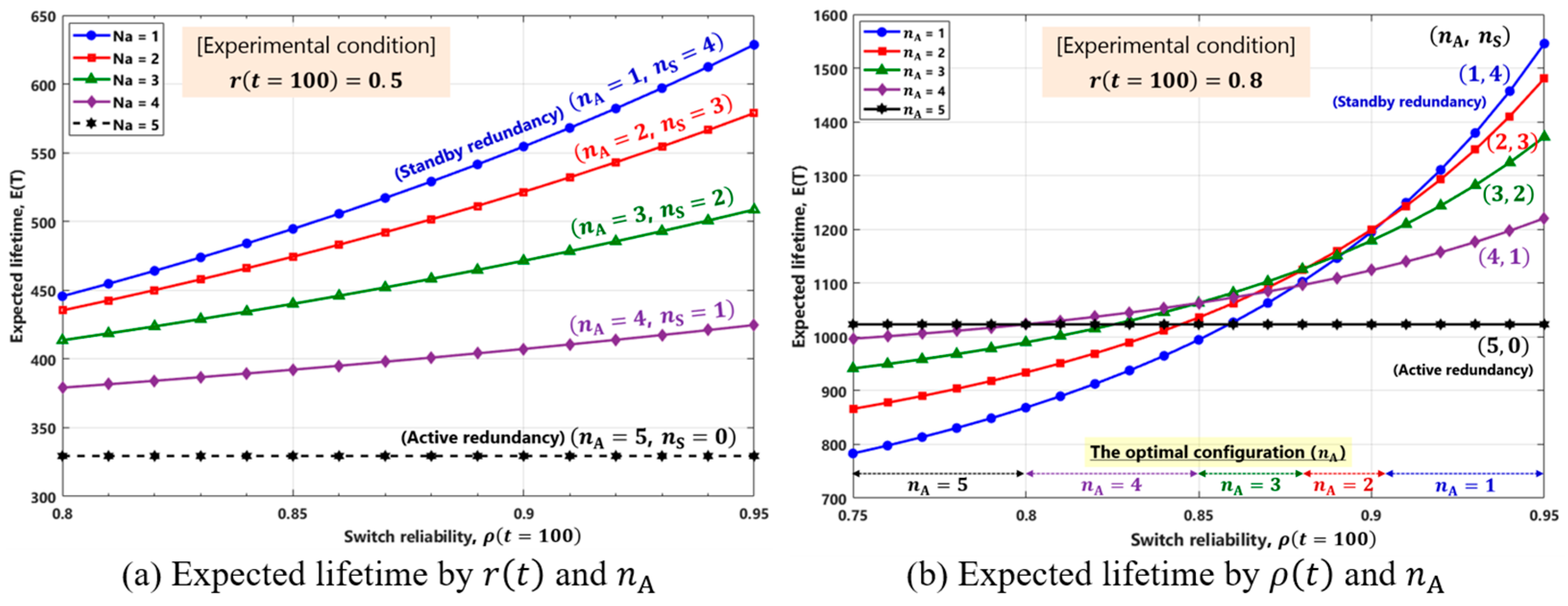
Figure 9 shows the observed expected lifetime, , of the mixed redundant system with five components as a function of the reliability of the components and switch. When the switch’s reliability, , is sufficiently more elevated than the reliability, , of the components, Figure 9a shows that the standby redundant system, , is the optimal configuration for the expected system lifetime (i.e., MTTF). Furthermore, as the number of standby redundant components increases, the growth rate, , of the expected system lifetime increases as increases. As shown in Figure 9b, when , the active redundancy strategy, , is recommended; however, the case of is not general. As increases, it is beneficial to increase the number of standby redundant components.

Figure 9.
Review the expected lifetime of a mixed redundant system.
4.2. Redundancy Allocation Problem (RAP)
This section presents the numerical experimental results on a well-known RAP benchmark. The experiments were conducted for two purposes: (i) to review the approximation error of the existing reliability function in Equation (2) for a mixed redundancy system; (ii) to observe the improvement in the system reliability through a mixed redundancy strategy, compared with other redundancy strategies, which are, ‘only active’ and ‘either active or standby’. The above two purposes are measured using the maximum possible improvement (MPI) index defined by Equation (18).
To maximize the system reliability at a designated mission time () within the upper bounds, and , of the system’s cost and weight, the RAP determines (1) the component type, (2) the number of redundancies, and (3) the number of active redundancies for each subsystem. Figure 10 shows the system configuration for the RAP benchmark. The benchmark system has 14 subsystems with 3 or 4 alternative components, as listed in Table 2. In Table 2, the TTF of the alternative component for subsystem is considered to be , and the cost and weight of the component are denoted as and , respectively. For all the subsystems, the TTF distribution of the switch for standby redundancy is supposed to be and , that is, . In addition, the upper limit on the number of components that can be installed in each subsystem is set to six, that is, for all .
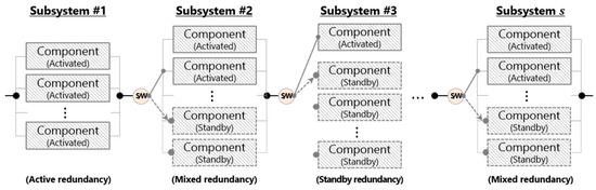
Figure 10.
Example (series–parallel) system for a RAP.
Table 2.
Component data for RAP example.
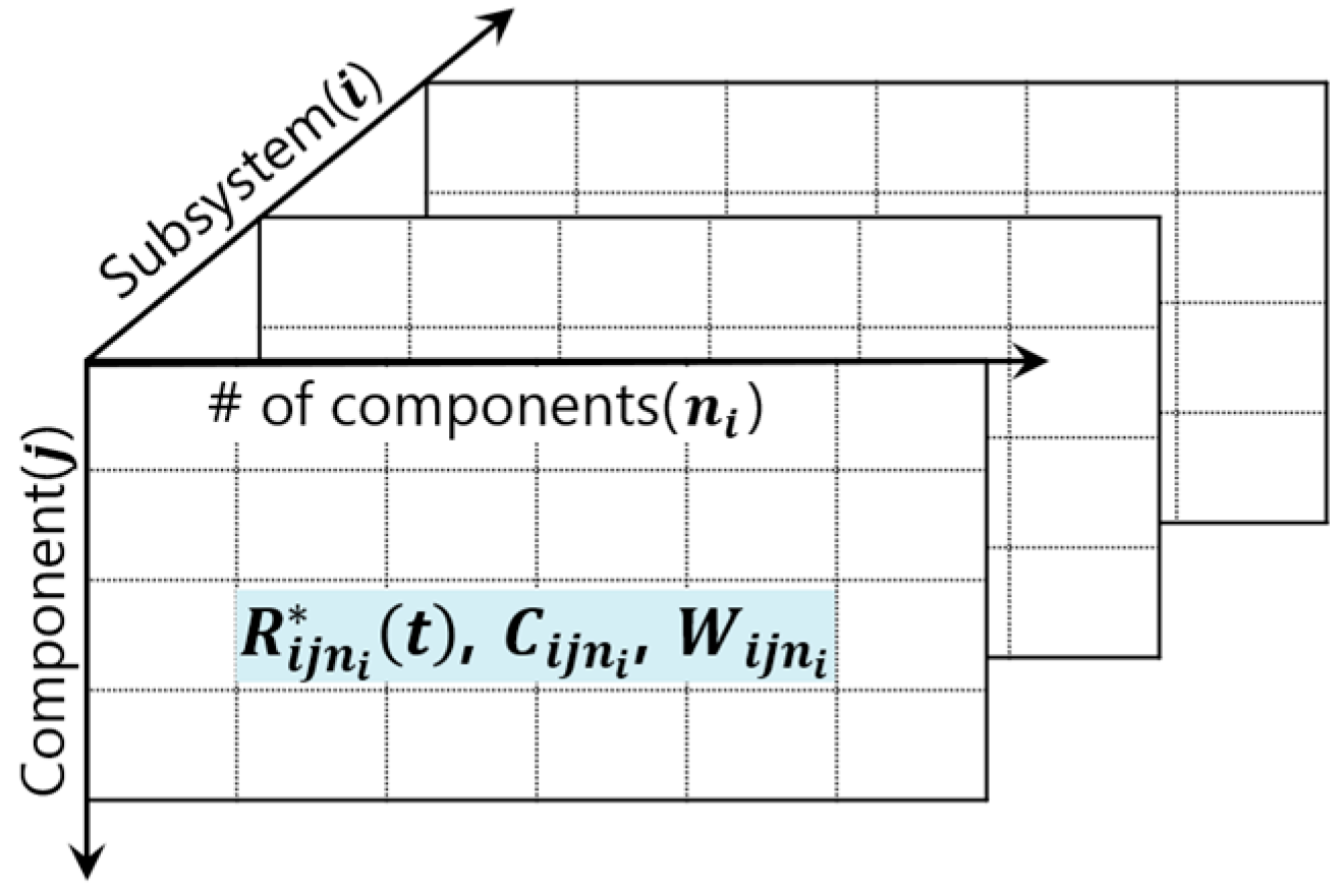
The RAP is presented as a nonlinear optimization problem with a nonlinear objective function for evaluating system reliability. However, to obtain optimal solutions for the RAP, it is necessary to convert this problem to a linear programming problem. Thus, in this study, the RAP is transformed into a simple binary integer linear programming problem, such as Equations (19)–(23), by constructing the three-dimensional matrices shown in Figure 11 through pre-calculation using MATLAB R2022a. In Figure 11, denotes the maximum reliability of subsystem when the component of the alternatives is selected and components are installed; namely, it is equal to . and represent the cost and weight of subsystem , respectively, with of the component, that is, and .
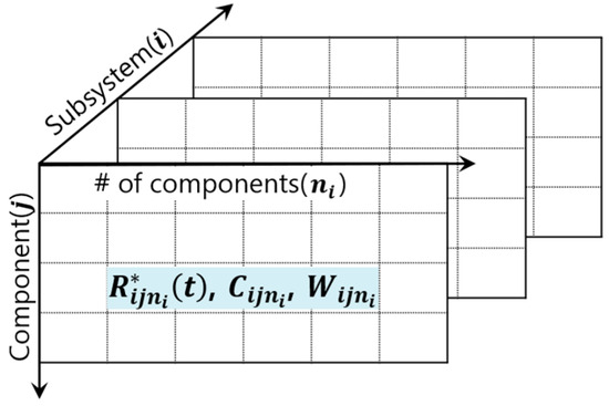
Figure 11.
Form of pre-computed data.
The objective function, Equation (19), maximizes the system reliability, and a logarithmic transformation is applied for linearization. Equations (20) and (21) constrain the upper limits of the cost and the weight of the system. Equation (22) indicates that the set for the type and number of components should be uniquely determined in the subsystem . Equation (23) indicates that the decision variable is a binary integer.
Table 3 shows the best solution of the RAP when , which was searched by Ardakan and Hamadani [17] using a genetic algorithm. Moreover, for each subsystem, Table 3 lists the approximated reliability by Equation (2), and the true reliability using Equation (14). A review of the approximation error of Equation (2) based on the MPI index showed that the average error is 15.0%, with a maximum and minimum of 24.5% and 3.4% at the 13th and 12th subsystems, respectively. When the subsystems are designed according to the best solution, the approximated and true values, and , of the system reliability are evaluated as 0.992329 and 0.993449, respectively, and the MPI index is 14.6%.
Table 3.
Approximation error of Equation (2) [17,23].
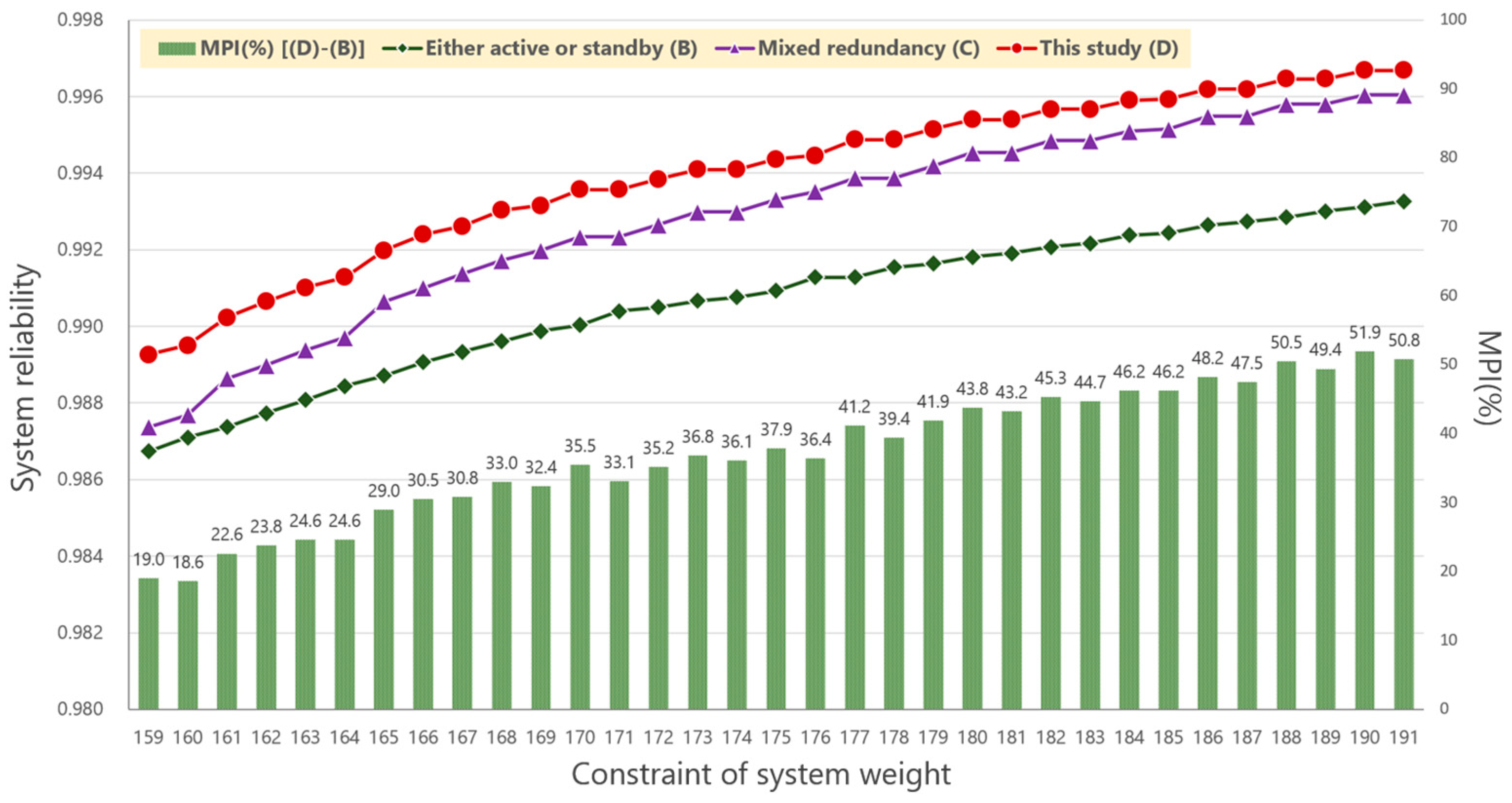
Moreover, numerical experiments for the above mathematical programming model, Equations (19)–(23), were conducted with 33 problems, while fixing the system cost () 130 and changed the system weight () from 159 to 191. The optimal solution for each system weight constraint was determined using ILOG CPLEX 20.1. The optimal reliability and structure of the system are presented in Table 4 and Table 5, respectively. Figure 12 visualizes Table 4, and the bar graph represents the MPIs for (D)–(B). In Table 4, the MPIs of (D)–(A) and (D)–(B) represent the system reliability improvement effect by considering the mixed redundancy strategy compared to ‘Only active (A)’ and ‘Either active or standby (B)’ strategies in the RAP. In the MPIs of (D)–(A), the average was 77.4%, with a maximum of 79.2% at and a minimum of 75.6% at . In the MPIs of (D)–(B), the average was 37.3%, with a maximum of 51.9% at and a minimum of 18.6% at . In conclusion, the mixed redundancy strategy is confirmed to implement a more reliable system than traditional strategies within equivalent resources.
Table 4.
Comparison of the optimal system reliability by the redundancy strategies considered.
Table 5.
The optimal system structure (, , ) by .

Figure 12.
The optimal system reliability by the redundancy strategies considered.
Furthermore, (C) in Table 4 shows the optimal system reliability of the RAP suggested by Sadeghi and Roghanian [21], based on Equation (2). The optimal system structures presented in Table 5 are identical to the configurations suggested in (C) [21], except for a slight difference when . At , the (C) recommended optimal configurations for the 1st and 12th subsystems as (3, 2, 1) and (4, 1, 1), respectively. Thus, the MPIs of (D)–(C) indicate the system reliability errors caused by Equation (2). The average MPIs was 15.6%, with a maximum of 16.5% at and a minimum of 14.0% at .
5. Conclusions and Future Study
This study suggests a lifetime distribution model for a mixed redundant system with an imperfect fault detector/switch. The proposed model is formulated by a structured CTMC that considers components’ TTF distribution as a generalized PHD. The PHD enhances the versatility and practicality of the model because it can represent diverse degradation patterns of the components exposed to varied operating environments. Also, the PHD can describe any random distribution well and represent all the distributions with finite support on non-negative integers [35]. Furthermore, the model provides accurate reliability by advancing the approximate reliability function suggested in the previous studies. It would be helpful in system design and management because it provides valuable information such as system reliability, hazard function, MTTF (i.e., expected lifetime), lifetime variance, skewness, and kurtosis based on the moment of the system’s lifetime distribution. Also, several insights for system reliability design are discovered in numerical experiments: (1) the mixed redundancy strategy implements a more reliable system than active and standby redundancies, and the effect of reliability improvement is more significant when the number of redundant components is reduced; (2) as the mission time required for the system expands, the mixed redundancy strategy is preferred over an active redundancy.
Based on this study, the following subjects could be recommended for future research. First, a structured CTMC model for a mixed redundant system with heterogeneous components needs to be developed, and component sequencing is also considered in the model [23,32,33]. Second, an optimization problem considering the system lifetime would be proposed, such as the expected lifetime, percentile lifetime, and expected residual lifetime [38,39,40]. Third, for a -mixed redundancy, a generalized form of mixed redundancy, it would be interesting to research a system lifetime model considering a PHD as the TTF distribution of components. Finally, developing a CTMC-based simulation methodology for a phased-mission system with a mixed redundancy strategy is recommended [41].
Author Contributions
Conceptualization, H.K.; methodology, H.K.; software, M.-K.B. and H.K.; validation, H.K. and M.-K.B.; formal analysis, H.K. and M.-K.B.; investigation, H.K. and M.-K.B.; resources, H.K. and M.-K.B.; data curation, H.K. and M.-K.B.; writing—original draft preparation, M.-K.B.; writing—review and editing, H.K.; visualization, H.K. and M.-K.B.; supervision, H.K.; project administration, H.K. and M.-K.B.; funding acquisition, M.-K.B. All authors have read and agreed to the published version of the manuscript.
Funding
This article was supported by “Regional Innovation Strategy (RIS)” through the National Research Foundation of Korea (NRF) funded by the Ministry of Education (MOE) (2021RIS-003).
Data Availability Statement
Data are contained within the article.
Conflicts of Interest
The funders had no role in the design of the study; in the collection, analyses, or interpretation of data; in the writing of the manuscript; or in the decision to publish the results.
References
- Coit, D.W.; Liu, J.C. System reliability optimization with k-out-of-n subsystems. Int. J. Reliab. Qual. Saf. Eng. 2000, 7, 129–142. [Google Scholar] [CrossRef]
- Jia, X.; Guo, B. Analysis of non-repairable cold-standby systems in Bayes theory. J. Stat. Comput. Simul. 2016, 86, 2089–2112. [Google Scholar] [CrossRef]
- Coit, D.W. Maximization of system reliability with a choice of redundancy strategies. IIE Trans. 2003, 35, 535–543. [Google Scholar] [CrossRef]
- Chen, T.C.; You, P.S. Immune algorithms-based approach for redundant reliability problems with multiple component choices. Comput. Ind. 2005, 56, 195–205. [Google Scholar] [CrossRef]
- Bhandari, A.S.; Kumar, A.; Ram, M. Grey wolf optimizer and hybrid PSO-GWO for reliability optimization and redundancy allocation problem. Qual. Reliab. Eng. Int. 2023, 39, 905–921. [Google Scholar] [CrossRef]
- Bhandari, A.S.; Kumar, A.; Ram, M. Hybrid PSO-GWO algorithm for reliability redundancy allocation problem with Cold Standby Strategy. Qual. Reliab. Eng. Int. 2024, 40, 115–130. [Google Scholar] [CrossRef]
- Jiang, Y.; Liu, Z.; Chen, J.H.; Yeh, W.C.; Huang, C.L. A novel binary-addition simplified swarm optimization for generalized reliability redundancy allocation problem. J. Comput. Des. Eng. 2023, 10, 758–772. [Google Scholar] [CrossRef]
- Mellal, M.A.; Zio, E. System reliability-redundancy optimization with cold-standby strategy by an enhanced nest cuckoo optimization algorithm. Reliab. Eng. Syst. Saf. 2020, 201, 106973. [Google Scholar] [CrossRef]
- Mellal, M.A.; Zio, E.; Al-Dahidi, S.; Masuyama, N.; Nojima, Y. System design optimization with mixed subsystems failure dependencies. Reliab. Eng. Syst. Saf. 2023, 231, 109005. [Google Scholar] [CrossRef]
- Zhang, J.; Lv, H.; Hou, J. A novel general model for RAP and RRAP optimization of k-out-of-n: G systems with mixed redundancy strategy. Reliab. Eng. Syst. Saf. 2023, 229, 108843. [Google Scholar] [CrossRef]
- Li, X.Y.; Li, X.; Feng, J.; Li, C.; Xiong, X.; Huang, H.Z. Reliability analysis and optimization of multi-phased spaceflight with backup missions and mixed redundancy strategy. Reliab. Eng. Syst. Saf. 2023, 237, 109373. [Google Scholar] [CrossRef]
- Hsieh, T.J. Performance indicator-based multi-objective reliability optimization for multi-type production systems with heterogeneous machines. Reliab. Eng. Syst. Saf. 2023, 230, 108970. [Google Scholar] [CrossRef]
- Mahdavi-Nasab, N.; Ardakan, M.A. Reliability optimization of multi-state consecutive sliding window systems under different activation strategies. Comput. Ind. Eng. 2023, 181, 109292. [Google Scholar] [CrossRef]
- Liang, Y.C.; Smith, A.E. An ant colony optimization algorithm for the redundancy allocation problem (RAP). IEEE Trans. Reliab. 2004, 53, 417–423. [Google Scholar] [CrossRef]
- Onishi, J.; Kimura, S.; James, R.J.; Nakagawa, Y. Solving the redundancy allocation problem with a mix of components using the improved surrogate constraint method. IEEE Trans. Reliab. 2007, 56, 94–101. [Google Scholar] [CrossRef]
- Tavakkoli-Moghaddam, R.; Safari, J.; Sassani, F. Reliability optimization of series-parallel systems with a choice of redundancy strategies using a genetic algorithm. Reliab. Eng. Syst. Saf. 2008, 93, 550–556. [Google Scholar] [CrossRef]
- Ardakan, M.A.; Hamadani, A.Z. Reliability optimization of series–parallel systems with mixed redundancy strategy in subsystems. Reliab. Eng. Syst. Saf. 2014, 130, 132–139. [Google Scholar] [CrossRef]
- Zio, E.; Gholinezhad, H. Redundancy Allocation of Components with Time-Dependent Failure Rates. Mathematics 2023, 11, 3534. [Google Scholar] [CrossRef]
- Talebitooti, R.; Gohari, H.D.; Zarastvand, M.R. Multi objective optimization of sound transmission across laminated composite cylindrical shell lined with porous core investigating Non-dominated Sorting Genetic Algorithm. Aerosp. Sci. Technol. 2017, 69, 269–280. [Google Scholar] [CrossRef]
- Katoch, S.; Chauhan, S.S.; Kumar, V. A review on genetic algorithm: Past, present, and future. Multimed. Tools Appl. 2021, 80, 8091–8126. [Google Scholar] [CrossRef]
- Sadeghi, M.; Roghanian, E. Reliability optimization for non-repairable series-parallel systems with a choice of redundancy strategies: Erlang time-to-failure distribution. Proc. Inst. Mech. Eng. Part O J. Risk Reliab. 2017, 231, 587–604. [Google Scholar] [CrossRef]
- Feizabadi, M.; Jahromi, A.E. A new model for reliability optimization of series-parallel systems with non-homogeneous components. Reliab. Eng. Syst. Saf. 2017, 157, 101–112. [Google Scholar] [CrossRef]
- Gholinezhad, H.; Hamadani, A.Z. A new model for the redundancy allocation problem with component mixing and mixed redundancy strategy. Reliab. Eng. Syst. Saf. 2017, 164, 66–73. [Google Scholar] [CrossRef]
- Dobani, E.R.; Ardakan, M.A.; Davari-Ardakani, H.; Juybari, M.N. RRAP-CM: A new reliability-redundancy allocation problem with heterogeneous components. Reliab. Eng. Syst. Saf. 2019, 191, 106563. [Google Scholar] [CrossRef]
- Sadeghi, M.; Roghanian, E.; Shahriari, H.; Sadeghi, H. Reliability optimization for non-repairable series-parallel systems with a choice of redundancy strategies and heterogeneous components: Erlang time-to-failure distribution. Proc. Inst. Mech. Eng. Part O J. Risk Reliab. 2021, 235, 509–528. [Google Scholar] [CrossRef]
- Reihaneh, M.; Ardakan, M.A.; Eskandarpour, M. An exact algorithm for the redundancy allocation problem with heterogeneous components under the mixed redundancy strategy. Eur. J. Oper. Res. 2022, 297, 1112–1125. [Google Scholar] [CrossRef]
- Ardakan, M.A.; Talkhabi, S.; Juybari, M.N. Optimal activation order vs. redundancy strategies in reliability optimization problems. Reliab. Eng. Syst. Saf. 2022, 217, 108096. [Google Scholar] [CrossRef]
- Abouei Ardakan, M.; Sima, M.; Zeinal Hamadani, A.; Coit, D.W. A novel strategy for redundant components in reliability-redundancy allocation problems. IIE Trans. 2016, 48, 1043–1057. [Google Scholar] [CrossRef]
- Ouyang, Z.; Liu, Y.; Ruan, S.J.; Jiang, T. An improved particle swarm optimization algorithm for reliability-redundancy allocation problem with mixed redundancy strategy and heterogeneous components. Reliab. Eng. Syst. Saf. 2019, 181, 62–74. [Google Scholar] [CrossRef]
- Hsieh, T.J. Component mixing with a cold standby strategy for the redundancy allocation problem. Reliab. Eng. Syst. Saf. 2021, 206, 107290. [Google Scholar] [CrossRef]
- Guilani, P.P.; Ardakan, M.A.; Dobani, E.R. Optimal component sequence in heterogeneous 1-out-of-N mixed RRAPs. Reliab. Eng. Syst. Saf. 2022, 217, 108095. [Google Scholar] [CrossRef]
- Guilani, P.P.; Juybari, M.N.; Ardakan, M.A.; Kim, H. Sequence optimization in reliability problems with a mixed strategy and heterogeneous backup scheme. Reliab. Eng. Syst. Saf. 2020, 193, 106660. [Google Scholar] [CrossRef]
- Peiravi, A.; Ardakan, M.A.; Zio, E. A new Markov-based model for reliability optimization problems with mixed redundancy strategy. Reliab. Eng. Syst. Saf. 2020, 201, 106987. [Google Scholar] [CrossRef]
- Kim, H.; Kim, P. Reliability models for a nonrepairable system with heterogeneous components having a phase-type time-to-failure distribution. Reliab. Eng. Syst. Saf. 2017, 159, 37–46. [Google Scholar] [CrossRef]
- Neuts, M.F. Matrix-Geometric Solutions in Stochastic Models: An Algorithmic Approach; Johns Hopkins University Press: Baltimore, MD, USA, 1981. [Google Scholar]
- Coit, D.W. Cold-standby redundancy optimization for nonrepairable systems. IIE Trans. 2001, 33, 471–478. [Google Scholar] [CrossRef]
- Buchholz, P. Structured analysis approaches for large Markov chains. Appl. Numer. Math. 1999, 31, 375–404. [Google Scholar] [CrossRef]
- Rykov, V.; Ivanova, N.; Kozyrev, D.; Milovanova, T. On Reliability Function of a k-out-of-n System with Decreasing Residual Lifetime of Surviving Components after Their Failures. Mathematics 2022, 10, 4243. [Google Scholar] [CrossRef]
- Azizi, S.; Mohammadi, M. Strategy selection for multi-objective redundancy allocation problem in a k-out-of-n system considering the mean time to failure. Opsearch 2023, 60, 1021–1044. [Google Scholar] [CrossRef]
- Devi, S.; Garg, H.; Garg, D. A review of redundancy allocation problem for two decades: Bibliometrics and future directions. Artif. Intell. Rev. 2023, 56, 7457–7548. [Google Scholar] [CrossRef]
- Li, X.Y.; Li, Y.F.; Huang, H.Z. Redundancy allocation problem of phased-mission system with non-exponential components and mixed redundancy strategy. Reliab. Eng. Syst. Saf. 2020, 199, 106903. [Google Scholar] [CrossRef]


Disclaimer/Publisher’s Note: The statements, opinions and data contained in all publications are solely those of the individual author(s) and contributor(s) and not of MDPI and/or the editor(s). MDPI and/or the editor(s) disclaim responsibility for any injury to people or property resulting from any ideas, methods, instructions or products referred to in the content. |
© 2024 by the authors. Licensee MDPI, Basel, Switzerland. This article is an open access article distributed under the terms and conditions of the Creative Commons Attribution (CC BY) license (https://creativecommons.org/licenses/by/4.0/).