Abstract
In the present study, we consider continuous-time modeling of dynamics using observed data and formulate the modeling error caused by the discretization method used in the process. In the formulation, a class of linearized dynamics called Dahlquist’s test equations is used as representative of the target dynamics, and the characteristics of each discretization method for various dynamics are taken into account. The family of explicit Runge–Kutta methods is analyzed as a specific discretization method using the proposed framework. As a result, equations for predicting the modeling error are derived, and it is found that there can be multiple possible models obtained when using these methods. Several learning experiments using a simple neural network exhibited consistent results with theoretical predictions, including the nonuniqueness of the resulting model.
Keywords:
Runge–Kutta method; ODE modeling; dynamics learning; modeling error analysis; stability analysis; Dahlquist’s test equation MSC:
68T07; 65L06; 65L09
1. Introduction
In the present study, we propose an analytical framework for modeling errors in modeling dynamics using discretization methods based on a linearization of the target dynamics. We also analyze the explicit Runge–Kutta methods in particular as the discretization method and show that the modeling results may not be uniquely determined when using these methods. (This paper is a revision of the preprint titled “An Error Analysis Framework for Neural Network Modeling of Dynamical Systems”, first available on 8 December 2021 at arXiv).
Assuming that the dynamics to be modeled are represented by a system of unknown ordinary differential equations (ODEs) of the form
we consider the modeling errors that arise in the modeling. In fact, dynamics in various fields are represented in this form, such as equations of motion in mechanics, state variable models in control, and models of chemical reactions of materials [1,2]. An important problem in modeling such dynamics is to obtain a continuous-time model:
where is constructed by some function approximation method such as neural network, Gaussian process, etc., from a sequence of observed data for a variable vector x of the system [3,4]. (The class to which belongs varies depending on each specific target dynamics and approximation method, but here, we assume that the method has the universal approximation property [5] for the class of ). If the time derivative of the variables of the system at each time in addition to x can be observed, then the determination of can be attributed to a regression problem [6], but there are situations in which such data are not available.
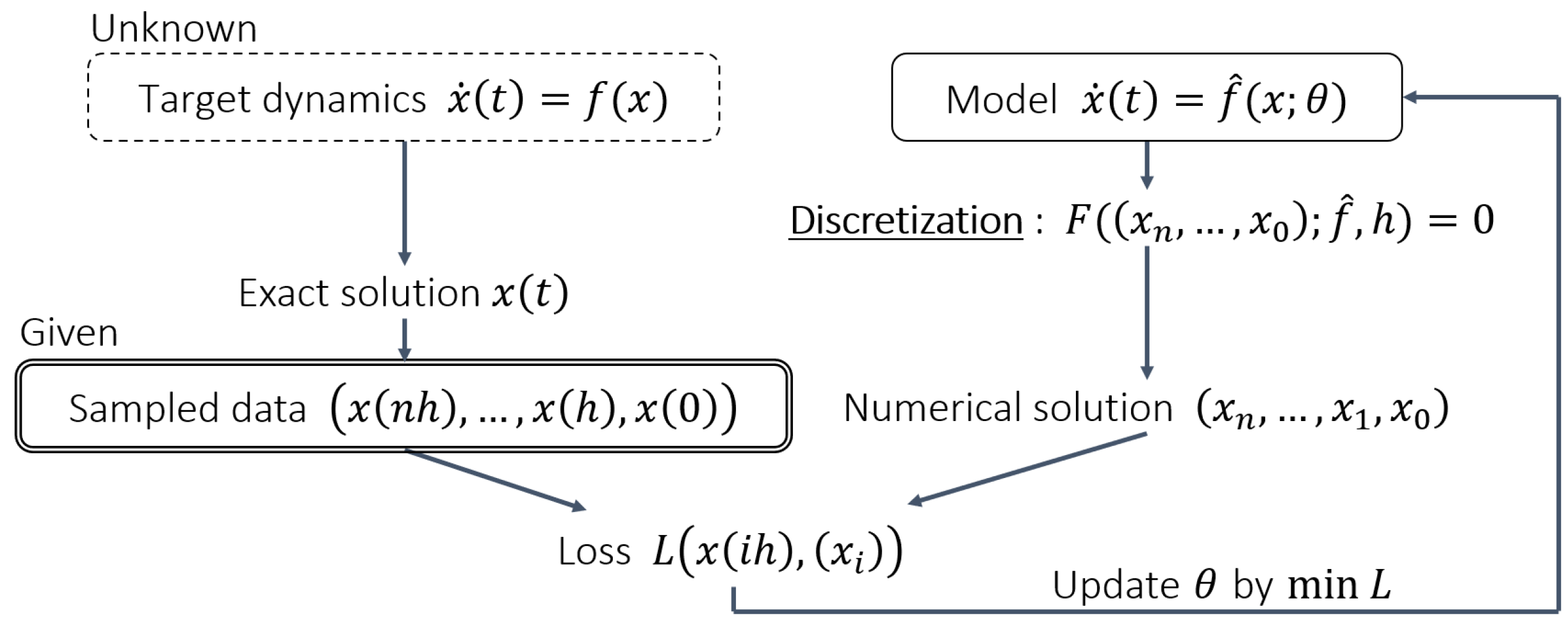
Therefore, as a method to construct the continuous model shown in Equation (2) without using the derivative values of the system variable, the numerical solution of the continuous model is computed, and then the model is indirectly optimized so that the numerical solution is as close as possible to the observed data [3,7,8,9,10,11,12,13,14,15,16,17,18,19,20,21,22,23,24]. The modeling procedure is briefly shown in Figure 1.
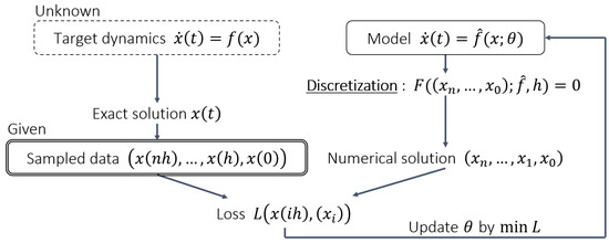
Figure 1.
An overview diagram of the modeling procedure. Model parameters are denoted by . The inputs of the loss function L are simplified for illustration.
Such a modeling approach can be said to use the discretization method in the opposite direction from the way it is normally used. Usually, when using and evaluating discretization methods, we consider the problem of finding an unknown discrete solution from a given ODE (we call this forward computation). On the other hand, when the discretization method is used in the modeling approach where the numerical solutions are compared with the observed data, the relationship between the ODE and the solution is reversed because the solution of the target system is given as observed data, and the ODE that defines the original unknown system is then approximated. Such an inverse relationship has not been considered in the usual numerical analysis [25,26,27]. In the present study, we propose a new evaluation framework of discretization methods for such inverse applications.
One of the early studies that proposed this type of continuous-time modeling approach was that of Rico-Martinez et al. in 1993 [12]. The possibility of combining the learning model with known continuous models is mentioned in some studies [16,20], which is difficult when using discrete-time models. An application for PDE is also studied [10]. In recent years, modeling methods focusing on the Hamiltonian structure of dynamics, which is characterized in continuous time, have been proposed [3,9,21]. (The loss function of Hamiltonian Neural Networks using finite difference can be considered the same as using the explicit Euler method.) In the existing studies on dynamics modeling, the key contribution to the performance of dynamics modeling is sought in the structure of the neural network [3,22] or the optimization method [15,16,19], and little attention is paid to the effect of the discretization method [9].
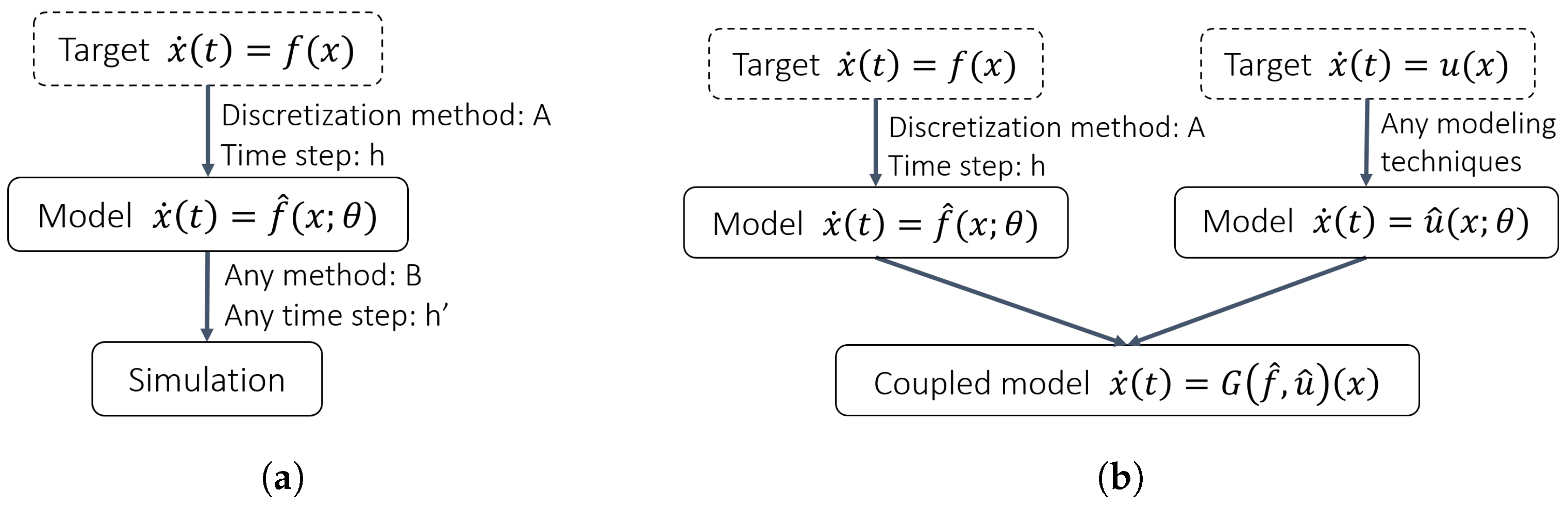
As shown in Figure 2, one of the advantages of the continuous models is that one can use a different discretization method and time step for the forward calculation to make predictions, and even couple the resulting model to other models modeled with different modeling methods, regardless of the methods used in the modeling process [12,15,19]. It is therefore desirable that the discretization process not be considered to be part of the resulting model and should affect the results as little as possible. In practice, however, there will be a modeling error that arises from the discretization process, i.e., the error between the original unknown dynamics f and in the continuous model shown in Equation (2).

Figure 2.
How continuous-time models are utilized. The model is used independently of the modeling method and can be integrated with different discretization methods and time steps, or coupled with other continuous models: (a) The independence of the methods used in modeling and simulation. (b) Coupling with other continuous-time models.
Several studies focus on the different discretization methods used for modeling. It is known that certain types of methods, such as implicit or linearly implicit methods, are suitable for the forward integration of stiff systems [26]. Rico-Martinez and Kevrekidis [12] and Oussar and Dreyfus [23] focused on the effectiveness of implicit methods for the integration of a stiff system [26], and they proposed to use implicit methods for the modeling of stiff target systems. Raissi et al. [17] and Chen et al. [24] compared the effectiveness of multiple discretization methods in the modeling task. However, these studies evaluate the difference in discretization methods mainly in terms of the prediction error (i.e., how close the model’s trajectory is to the target dynamics) or noise robustness.
An important study that directly addresses the error between the target and the model is presented by Zhu et al. [9] In the study, the error between the two is distinguished as the “target error” from the other errors introduced in the optimization, generalization, and approximation processes. The concept is extended to more general target dynamics and discretization methods in later studies [7,8], allowing an order evaluation of the target error using the formally defined equation named inverse modified differential equations (IMDE), which is identified with the modeled dynamics.
The IMDE-based analysis method by Zhu et al. is general and rigid. However, if one can directly know how the nature of the specific target dynamics (i.e., oscillatory, dissipative, divergent) affects the error, it becomes easier to appropriately choose or design the discretization method to be used for the modeling of the target dynamics. A successful example of analyzing discretization methods with a focus on the nature of dynamics is the stability analysis of discretization methods [26,27,28]. In this study, we propose an error analysis framework of discretization methods used in the modeling purpose following the concept of the stability analysis.
A more detailed description of the problem setup and the definition of the modeling error in the present study is given below. To represent the nature of the target dynamics, we formulate the modeling error using Dahlquist’s test equation, referring to the stability analysis of the discretization method [26,27,28]. Dahlquist’s test equation is an approximation of the target dynamics for estimating the result of the modeling process, in the sense that it is obtained by linearizing the equation of dynamics and considering the Jordan canonical form. If a rough distribution of modes of the target dynamics is known, e.g., using DMD [29], the results for the test equations corresponding to such modes can be used to estimate the modeling error for the target dynamics. In addition, Dahlquist’s test equation is characterized by a single complex parameter, allowing the properties of the discretization method to be examined graphically in the complex plane, as is carried out in the stability analysis.
As a main result, we derived an equation that is satisfied by the learned model when the model perfectly reproduces the sampled solution of the test equation using an explicit Runge–Kutta method. The solution of the equation predicts the resulting model, and we used it to define the modeling error.
One important result is that the above equations for more than two-stage explicit Runge–Kutta methods have multiple solutions. (A similar result is addressed in an analysis example for a composite method of the explicit Euler method in the work by Zhu et al. [7].) This means that the modeling results may not be uniquely determined. This is not only a potential problem in practical modeling, but it also makes the design of explicit Runge–Kutta methods for modeling purposes difficult.
In order to confirm the validity of the theoretical considerations, learning experiments are conducted using the explicit midpoint method, a two-stage Runge–Kutta method, for test equations with various parameters. A multilayer perceptron, a simple neural network, is used as the learning model. The results confirm that any of the expected results are reproduced and that the nonuniqueness described above occurs in some cases.
Remark 1.
The family of Runge–Kutta methods, especially the four-stage, fourth-order explicit Runge–Kutta method (the classic Runge–Kutta method; RK4), is a very widely used discretization method in forward computation and is also implemented in various ODE solvers. With this background, the Runge–Kutta method is considered a natural candidate for modeling. In fact, a learning model composed of neural networks is discretized and trained using the classic Runge–Kutta method in many studies [12,15,18,19], and related research explicitly uses Runge–Kutta in the name of modeling architectures, e.g., Runge–Kutta Neural Networks (RKNNs) [13,15,22]. However, when a Runge–Kutta method is used for modeling as described above, it is shown in the present study that there are multiple possible models that reproduce the same observed data. Among such models, some may approximate the dynamics of the target well, while others may not. This may not be a problem when the model is used as a discretized model that assumes the same time step as the observed data, but this can lead to undesirable results when used as a continuous model.
2. Modeling Error Analysis
2.1. The Test Equation
Dynamics expressed in the form of Equation (2) range so widely that it is not easy to define the modeling error for all of them. Therefore, as a representative of these various dynamics, we use one-dimensional dynamics called Dahlquist’s test equation [26,28]:
The test equation can be thought of as a linearized and diagonalized form of general dynamics.
The test equation is characterized by a complex parameter . The dynamics expressed by the test equation are more damped the more is negative, and the oscillation becomes more intense for larger values of .
Instead of examining modeling errors for various f, we examine modeling errors for the test equations at various . That is, we define the modeling error parameterized by the complex number . By examining the modeling errors for various , we can see what dynamics the method is suitable for modeling. Conversely, by studying the modeling errors for various for various discretization methods in advance, it is possible to determine which discretization method is suitable for modeling based on prior knowledge of the rough mode distribution of the dynamics to be modeled. Moreover, it can be applied not only to evaluate existing discretization methods but also to design discretization methods that minimize modeling error for within a specified region [30].
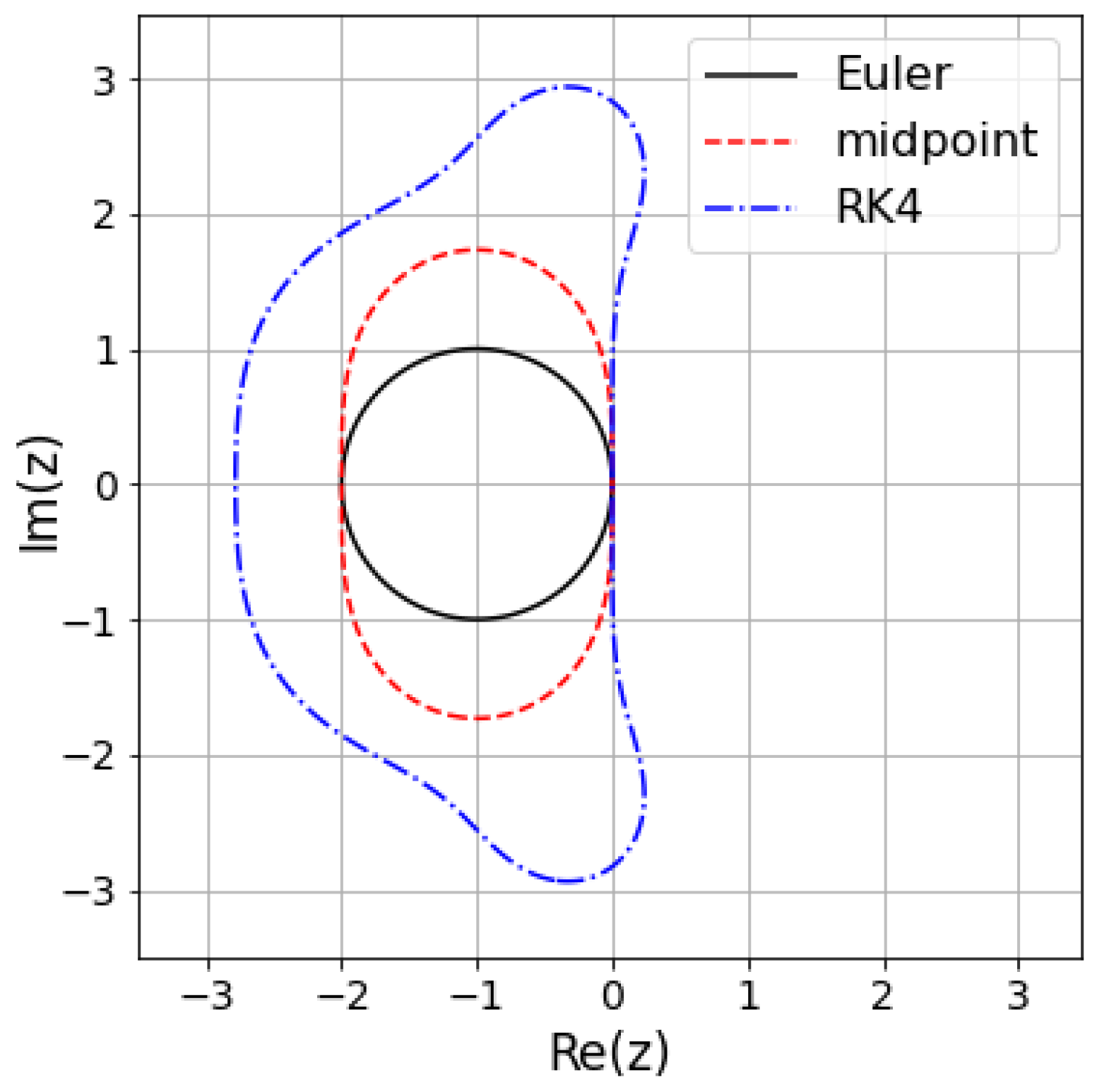
The test equation has been used to analyze the stability of discretization methods. Figure 3 shows the results of the stability analysis for some methods. It shows that the dynamics by s in the region inside the plotted line can be integrated stably by the method and the time step h. The idea of the present study is analogous to the stability analysis in that the test equation is used as a sort of benchmark for the analysis, and the properties of the discretization method are represented on the complex plane.
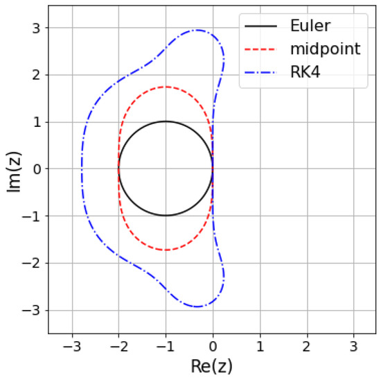
Figure 3.
An example of the stability analysis. The stability regions for the explicit Euler method (Euler), the explicit midpoint method (midpoint), and the classic fourth-order Runge–Kutta method (RK4) are shown. The parameter of the test equation is normalized by the time step h as .
2.2. Continuous Modeling of Dynamics with Observed Data
In the present study, we investigate modeling errors when modeling the target dynamics with ordinary differential equation models. Modeling here refers to the assuming that the dynamics to be modeled is an ordinary differential equation:
and approximating the function f on the right-hand side using observed data of the dynamics. That is, we consider the problem of optimizing the model so that the solution of the ordinary differential equation model:
reproduces the observed data considering the data to be a sampling of trajectories of Equation (4).
Since it is generally difficult to directly observe the derivative of a variable in a system, we assume that is not included in the observed data. Under such an assumption, we cannot directly optimize as a regression problem in the space of maps mapping x to . Therefore, we discretize using a discretization method (in particular, an explicit Runge–Kutta method) and introduce a map from the space X of variables x to X that depends on , thereby optimizing using only observed data on X.
Let the set of observed data consisting of m trajectories be denoted as follows:
where is the exact solution of (4) for the initial value and each of those trajectories is denoted by . The observed data are assumed to be sampled at equally spaced intervals with step size h, and the effect of noise is ignored. Here, n is the number of sample points in a trajectory, which is equal to the number of steps in the discretization method used for modeling.
Remark 2.
If the observed data consist of trajectories with more steps than the discretization method, they can be split into smaller subtrajectories to apply this modeling method. Since this study considers the ideal case where n-step trajectories from any initial value can be completely modeled, considering n-step trajectories for n-step methods by patching n-step results taking the points in the middle of the trajectory as initial values is sufficient.
Using such observed data, we optimize the model shown in Equation (5). Optimization is performed so that the observed data in each trajectory match the numerical solution of the model. Let
denote an equation that defines a discretization method (n-step method) for an ODE . g in the definition of the method is a vector field, which is given and integrated into the traditional forward application of the method. In the modeling process, substitute g with , the model to be optimized, and consider the following optimization problem:
Note that is an appropriate norm on X. We call
the objective function or loss function.
Example 1.
Since F for the explicit midpoint method (see Section 3.1)
can be written as
the optimization problem (8) becomes
Example 2.
For the implicit Euler method, F is represented as
2.3. Modeling Error
Suppose that the modeling process described in the previous section yields that perfectly reproduces the observed data. Even in such an ideal case, f and do not necessarily coincide due to the effect of discretization, and the error depends on both the discretization method and the nature of the target dynamics f. In this section, we formulate such an error as a modeling error and propose a new evaluation criterion for discretization methods.
In defining the modeling error, as is performed in the stability analysis of numerical methods, we consider the results of modeling when using the test Equation (3) as a representative of target dynamics f. We also make two idealized assumptions to investigate certain limits of the optimization problem (8). First, assume that a sufficient amount of data are available and that can be learned such that the objective function (9) is zero for any , a sampling of the exact solution with a step size h. That is, for any initial value of , the following holds:
Furthermore, we assume the universal approximation property [5] for the construction of . Thus, there exists an that reduces the objective function to as close to 0 as desired. Among such s, when there exists a linear in particular, the modeling error is defined as follows:
Although there may be other models that reduce the loss function to 0, we assume in particular a result of the form (16) because this is an ideal case in the sense that it belongs to the same class as the test equations, i.e., the modeling target.
Remark 3.
As discussed in Theorem 1, if using explicit Runge–Kutta methods, there exists a linear such that the objective function becomes 0.
Definition 1
(Modeling Error). For such that the objective function (9) reduces to 0, define the learnability coefficient ℓ as follows:
Errors for the real and imaginary parts are also defined in the same way as the modeling error.
Definition 2.
For such that the objective function (9) reduces to 0, define the modeling error with respect to the real part and the modeling error with respect to the imaginary part as follows:
Remark 4.
These two types of modeling errors (ℓ and, or ) are intended for different uses. The overall error ℓ is useful for designing discretization methods, whereas the component errors are useful for analyzing the effectiveness of existing discretization methods for given dynamics.
The characteristics of various discretization methods can be compared by illustrating on the complex plane the dynamics that result in a small modeling error for each given discretization method.
Definition 3.
If the modeling error ℓ can be written as a function of , define the learnability region for a given discretization method with an acceptable error by the following:
In addition, the learnable region for the modeling error of real and imaginary parts is defined in the same way.
Remark 5.
Note that although the constant 1 that appears in the inequality in the definition of the stability region in the stability analysis has meaning as a limit with respect to divergence, the tolerance in the learnable region has no special meaning. Basically, a smaller modeling error is better, and it is important to investigate the learnability regions by changing ϵ to 0.1, 0.01 (10%, 1% error allowed), and so on, depending on the error allowed for each application.
3. Analysis of Explicit Runge–Kutta Methods
3.1. Explicit Runge–Kutta Methods
The explicit s-stage Runge–Kutta methods for an initial value problem
are given by
where and are real coefficients that determine the method.
Lemma 1.
The explicit Runge–Kutta methods for the test equation can be expressed as
where
Proof.
By definition, the following holds for k:
This can be transformed as . Since the Runge–Kutta method is explicit, the matrix becomes a lower triangular matrix with nonzero diagonal elements. Therefore, exists for any h and , and k and can be expressed as
□
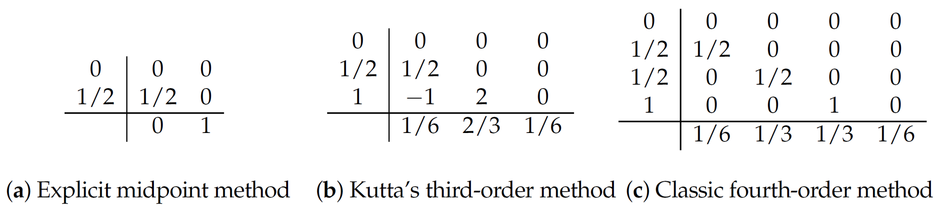
Example 3.
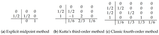
The explicit midpoint method, Kutta’s third-order method, and the classic fourth-order method are expressed as in Figure 4 using the table-like notation of A, b, and c (the Butcher Tableau [25,31]):
Since we assume the target dynamics to be time-independent, the c vector in the standard Butcher tableau can be ignored.
Figure 4.
Examples of explicit Runge–Kutta methods.
3.2. Idealized Prediction Equation
For a given explicit Runge–Kutta method (21), an equation satisfied by the linear model that makes the objective function 0 is derived, leading to the existence of such a model.
Theorem 1.
Let a discretization method for Dahlquist’s test equation ( be an explicit s-stage Runge–Kutta method . Let D a set of 1-step trajectories of the test equation starting from initial points as:
where m is a positive integer. Denote the learning model as
When learning the test equation by considering an optimization problem
where the loss is
and
is the equation of the Runge–Kutta method for the model, there exists a model
such that for any trajectories D, satisfying the following:
Proof.
Assume that we have a model . With Lemma 1, the equation of the method is as follows:
Therefore, the optimization problem becomes
Factoring out , we obtain
If there exists satisfying (32), then Equation (35) is zero for any sampled trajectories D of the test equation with a step size h. Since (32) is a polynomial of , such a exists by the fundamental theorem of algebra. □
Definition 4.
We call Equation (32) the learnability equation of the Runge–Kutta method and the left-hand side of the equation is referred to as the learnability polynomial.
The learnability equation describes the ideal result of modeling for the target and the Runge–Kutta method used, in the sense of the optimization problem (8).
Remark 6.
The parameter λ, which represents the target dynamics, appears as the term in the learnability equation. Note that the solution of the learnability equation is periodic with respect to λ in the direction of the imaginary axis by .
Corollary 1.
In general, the learnability polynomial of an s-stage Runge–Kutta method is an s-order polynomial of , and thus the learnability equation has s solutions. Therefore, the resulting model may not be uniquely determined by the optimization problem (8). See Section 3.3 for details.
Example 4.
The learnability equation for the explicit midpoint method is
and it has two solutions
For the modeling error ℓ of the explicit Runge–Kutta methods, the scaling law with respect to step size h holds, as in the stability analysis. This is an important property for the modeling error to serve as an evaluation metric for discretization methods.
Theorem 2.
The modeling error of the explicit Runge–Kutta methods
is a function of .
Proof.
From the learnability equation, we have
and substituting yields
This shows that the solution , and also , is a function of z. □
The same holds for the component-wise modeling error.
Theorem 3.
The component-wise modeling errors for the explicit Runge–Kutta methods are functions of and .
Proof.
We prove this for . The same goes for .
If is a solution of the learnability equation for , then is also a solution of the equation for . Thus, as in the proof of Theorem 2, is a function of . Since in the definition of can be transformed as
it follows that is a function of z and . □
3.3. Nonuniqueness of Modeling Results
As mentioned in Theorem 1, the learnability polynomial for the explicit s-stage Runge–Kutta methods is a polynomial in and thus has s roots. Each of these roots is a parameter that characterizes the linear model obtained as a result of modeling, meaning that there can be more than one candidate among the linear models. In modeling in the sense of the optimization problem (8), even if a model can be learned such that the loss is zero, the result is not expected to be uniquely determined. On the other hand, this is not considered to be a critical issue in learning a discrete model, since the same result can be obtained as a one-step flow map regardless of which solution is chosen.
This nonuniqueness is caused by the fact that in modeling with the Runge–Kutta method, multiple compositions of the unknown function are optimized with only one step of the discrete solution. The point is that, whereas the performance of forward calculation is improved by applying a known function multiple times, in modeling, the composition of an unknown function increases a certain degree of freedom, making it impossible to determine with only one step of observation data.
Remark 7.
In actual learning, some selectivity may occur in the learning results depending on the structure of the specific learning model and the optimization method used in the learning process. The selectivity here refers to the difference in learnability among multiple λ for a target λ. For example, the following are possible criteria for selectivity, but it is not clear that selectivity necessarily arises based on such easily interpretable criteria:
- Degree of approximation (some distance to the target λ).
- Closeness to the origin.
It is necessary to examine and analyze the models and algorithms used for each individual case.
3.4. Minimum Modeling Error
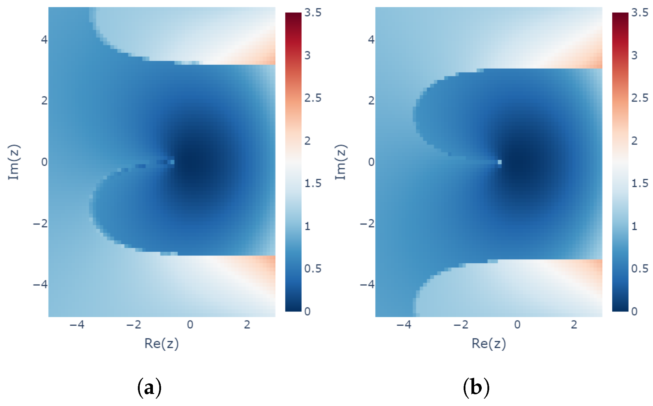
In this section, we consider the most desirable result to be that which is closest to among the candidate s. Specifically, we examine the modeling error for the solution of the learnability equation that has the smallest value of . This is the with the smallest modeling error, and, in this sense, it is the most desirable result. At the same time, it also provides a lower bound on the modeling error as a limitation of optimization in the sense of (8).
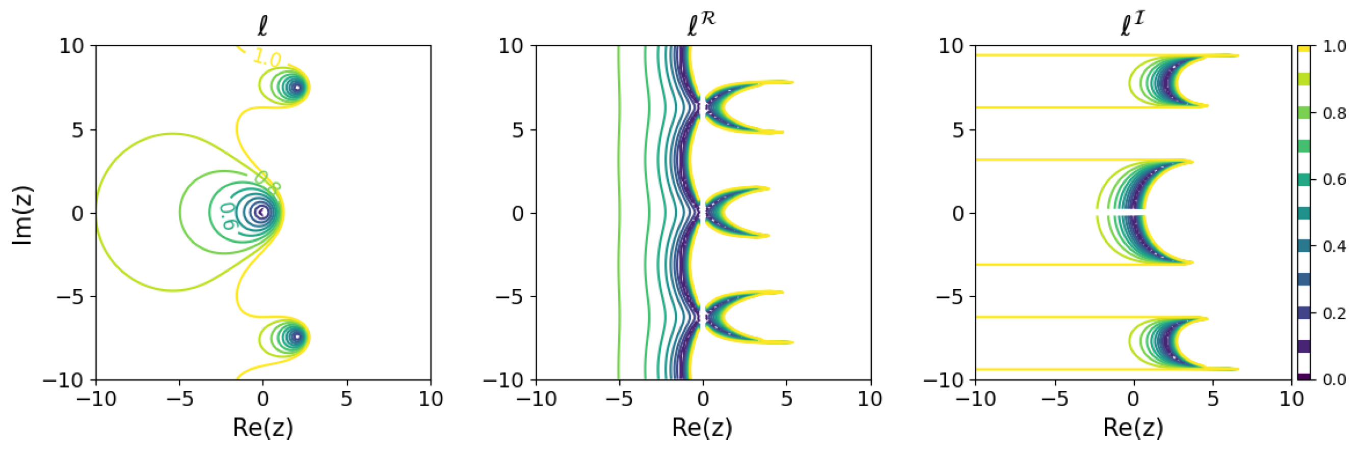
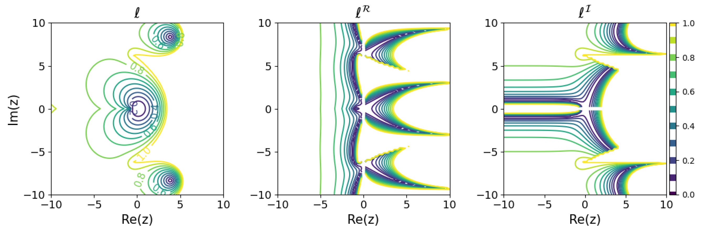
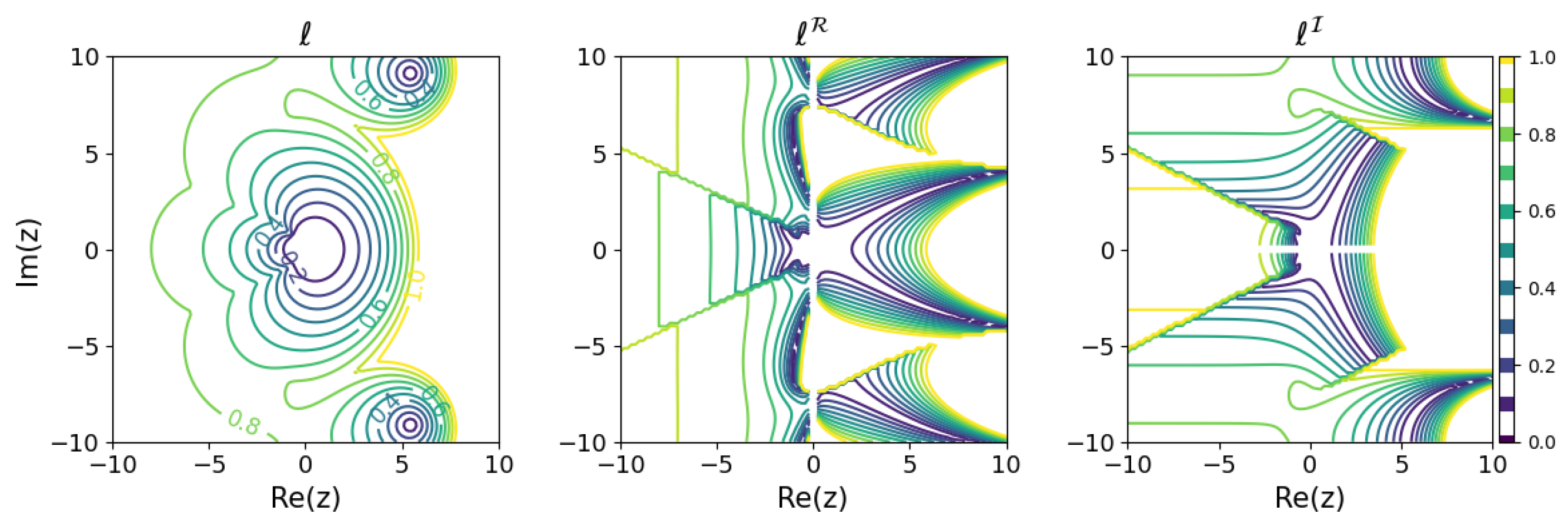
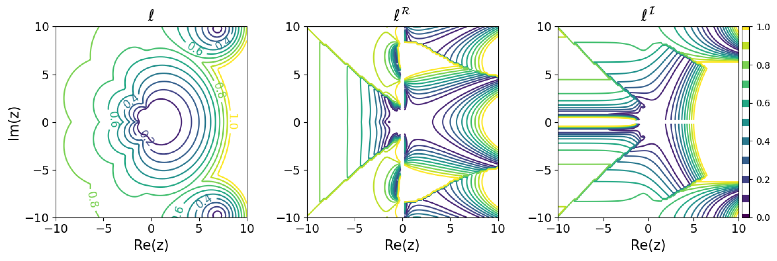
The results for several Runge–Kutta methods are shown in Figure 5, Figure 6, Figure 7 and Figure 8. The and modeling error based on the above criterion were calculated for on a grid with 0.2 ticks in a rectangular region on the complex plane and are plotted in contour plots. For visibility, only portions with a modeling error of 1 or less are colored. In order to find such s, all solutions of the learnability equation were calculated numerically for each , and then the smallest of was chosen.
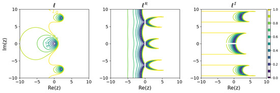
Figure 5.
Minimum learnability coefficients for the explicit Euler method.
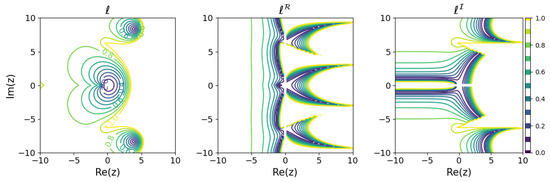
Figure 6.
Minimum learnability coefficients for the explicit midpoint method.

Figure 7.
Minimum learnability coefficients for Kutta’s third-order method.
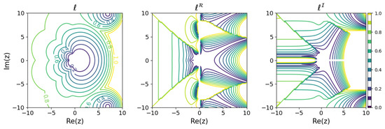
Figure 8.
Minimum learnability coefficients for the classical fourth-order method.
These results show that the higher the order of the Runge–Kutta method, the wider the region of small modeling error near the origin. On the other hand, looking locally, there are regions where the relationship between the order of the Runge–Kutta method and the modeling error is inverted. For example, comparing the explicit Euler method with the explicit midpoint method, for purely decaying dynamics in the negative region on the real axis, even if a is obtained that minimizes the modeling error, the explicit Euler method could yield a model with less error than the explicit midpoint method. Although, intuitively, it would seem that a higher-order method would be more appropriate for modeling, it turns out that there are cases in which a lower-order method should be used, depending on the dynamics of the modeling target.
4. Learning Experiment
4.1. Targets
In Section 2 and Section 3, we proposed a modeling error analysis for discretization methods and predicted the results when using the explicit Runge–Kutta methods. In this section, we verify whether any of the predicted results can actually be obtained, and whether nonuniqueness appears, by conducting learning experiments using simple neural networks. Specifically, the explicit midpoint method, which is a two-stage explicit Runge–Kutta method, is used as one of the simplest of the Runge–Kutta methods that could yield multiple modeling results, and the test equations by in a specific region of the complex plane are learned. The resulting model is then approximated as linear and is compared with the original . The dynamics to be trained was on grid points satisfying . The time step size h was set to 1. For each of these , was learned independently.
4.2. Model and Method
In this learning experiment, a neural-network-based learning model, , the multilayer perceptron (MLP), was used. This is a simple and basic neural network, and there is no elaboration on learning the test equations.
The learning model consists of three layers: an input layer, a hidden layer, and an output layer. In order to learn a mapping from complex to complex, the input and output layers both have two real elements corresponding to the real and imaginary parts, respectively. The hidden layer is a fully connected layer with a width of 200 nodes. ReLU is used as the activation function inserted between each layer. The overall structure can be summarized as follows: a linear layer with 200 outputs from two inputs, ReLU, a linear layer with 200 outputs from 200 inputs, ReLU, and a linear layer with two outputs from 200 inputs.
The training data consist of pairs of initial points and one-step solution . The real and imaginary parts of the initial point are independently produced by uniform random numbers with values in , and is regarded as sampled from a rectangular region in the complex plane. The training data set D is a set of 5000 pairs of and with . The test data are generated in the same way, using 5000 pairs of data.
The seed of the random numbers is increased by 1 each time the is changed. Random numbers are used to initialize the parameters of the learning model. Therefore, when a common phenomenon is obtained for each as a result of the experiment by fixing the seed, it is difficult to distinguish whether the results are similar because of the same initial values or whether the results are really independent of (such as selectivity of caused by the structure of the neural network).
For an optimizer, we used the Adam method with a learning rate of 0.001. We trained a total of 10,000 epochs, with one epoch being a batch training using all of the training data at once. The loss is saved every 100 epochs.
4.3. Estimation of
The definition of the modeling error assumed that a linear model is obtained as a result of learning. However, general learning models, including the MLP described in the previous section, are nonlinear, and the quantity corresponding to may not be obtained directly.
Therefore, in this experiment, the input–output ratio of the training model is averaged over the range of the initial point used for training, and the subsequent analysis is performed by considering it as . That is, the average , defined as
is used as an estimation of , where E is the set of for evaluating the input–output ratio, and M is the number of its elements (evaluation points). As E, we used on a grid of 20 points each in the real- and imaginary-axis directions from the range , for a total of points.
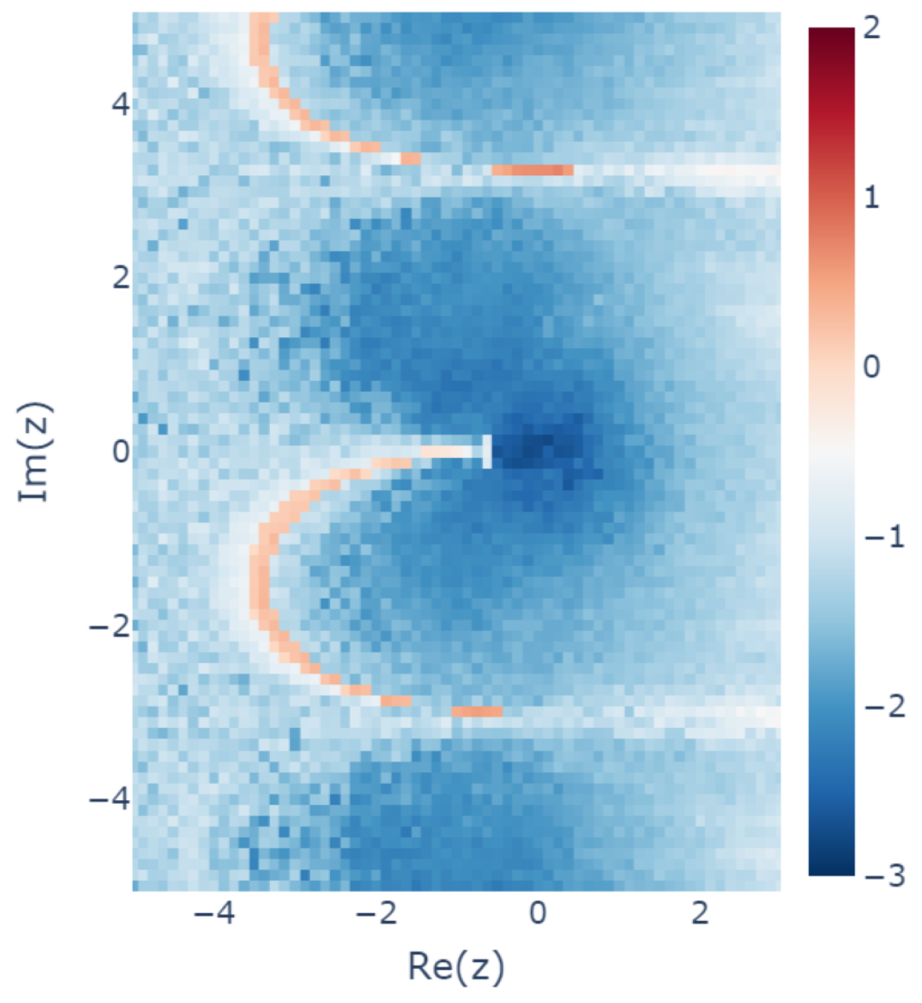
The experimental results confirm that the learned model was close to linear functions for most of the . For each , the standard deviation of the input-output ratio with respect to was calculated, and its common logarithm plotted in the z plane is shown in Figure 9 (the first case in Section 4.4.1, where the seed is incremented from 0). The smaller the standard deviation, the closer the input–output ratio is to a constant independent of , indicating that the model is almost linear. However, the standard deviation is relatively large for on the semicircle in the third quadrant. This is located at the boundary of the nonuniqueness region (see Section 4.4.2) and is considered to be a difficult region to learn for some reason.

Figure 9.
Heatmap of the standard deviations of the input-output ratios for for each z plotted with the common logarithm scale, using the results for the case of “Seed from 0”, as described in Section 4.4.1. Smaller values indicate that the model can be considered to be linear.
4.4. Results
4.4.1. Comparison with Theoretical Prediction
Figure 10 shows the modeling errors computed from the learning results for the two cases with different seeds. The modeling error calculated with estimated by the learned for each is plotted on the z-plane. In both cases, the seeds are incremented by 1 for each different . In the first case, the seed is set to 0 for and for , and, in the second case, the seed is set from 1 to .

Figure 10.
Learnability coefficients of the learned MLP model using the explicit midpoint method. Different random seeds are used for the two experiments: (a) Random seed incremented from 0 (for lower-left z) to (for upper-right z). (b) Random seed incremented from 1 (for lower-left z) to (for upper-right z).
This plot shows that the learning results near the origin are in good agreement with the minimum modeling error expected in Figure 6. A discontinuous surface appears around , which is considered to be a result of the periodicity of due to the learnability equation having z in the form . Note that there are regions in which different are learned when the seed of the random number is changed. This nonuniqueness is considered to correspond to the existence of two solutions to the learnability equation for the explicit midpoint method (see Section 3.3).
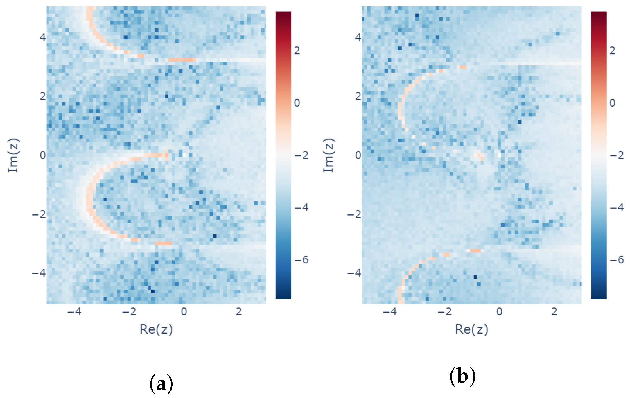
Next, we verified that the results were those predicted by either of the two solutions of the learnability equation. For this purpose, the minimum absolute value of the difference between the modeling error of the training result and the modeling error expected from the two solutions (see Equation (36)) was calculated for the training results of both cases as
Figure 11 shows the error , which was confirmed to be small.
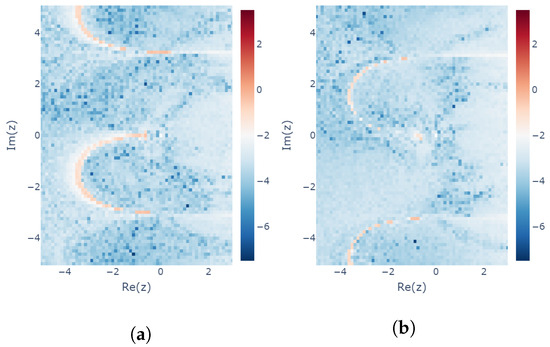
Figure 11.
Heatmap of the prediction error of the modeling error for the explicit midpoint method. The logarithms of the error (see Equation (41)) are plotted: (a) Seed incremented from 0 (for lower-left z) to (for upper-right z). (b) Seed incremented from 1 (for lower-left z) to (for upper-right z).
4.4.2. Variation in Nonunique Results
In order to further examine the variation of the results, we conducted the same experiment with 28 different sets of seeds following the previous two cases (30 in total) as 2 to , 3 to , …, and 29 to . Then, for each case, we examined which of the two solutions of the learnability equation was learned. The distance between the expected results and and the actual result was calculated for each in each case and was labeled if was close to and if was close to . Figure 12 shows the results of calculating the standard deviation of the 30 labels for each . If the standard deviation is 0, then the result is unique, and if the standard deviation is large, then different results are trained for different seeds.
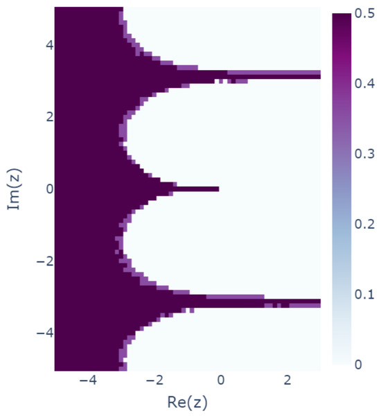
Figure 12.
Variation in the results with different seeds. Results for which is closer to are labeled 1, and results for which is closer to are labeled . Then, the standard deviations of the labels are plotted.
This analysis reveals that the learning results are nonunique with a large standard deviation, especially in the boundary region of the periodicity and in the region in which the real part of z is negative to some extent. This shows that the actual learning outcome may not be uniquely determined, as theoretically expected. The standard deviation was close to 0.5, indicating that and were learned randomly without bias. The cause of this phenomenon could be the structure of the model used for training or the optimization method used, but further discussion is left for future study.
5. Conclusions
In the present study, a framework for investigating modeling errors caused by the discretization method used for the continuous-time modeling of dynamics is proposed. As a specific result of the analysis using the proposed framework, an equation that predicts the results when an explicit Runge–Kutta method is used for modeling is obtained. It was shown that even if a model that perfectly reproduces the observed data is obtained, then there is a nonzero lower bound on the modeling error and that more than one model can be obtained. Furthermore, training experiments using a multilayer perceptron confirmed that nonuniqueness of results does in fact occur. Future study will include clarification of the cause of the nonuniqueness observed in the learning experiments and analysis of the modeling error for a system with inputs.
Author Contributions
Conceptualization, T.Y.; methodology, S.T.; software, S.T.; validation, S.T.; formal analysis, S.T.; investigation, S.T.; writing—original draft preparation, S.T.; writing—review and editing, S.T. and T.Y.; visualization, S.T.; supervision, T.Y.; project administration, T.Y.; funding acquisition, T.Y. All authors have read and agreed to the published version of the manuscript.
Funding
This research is supported by JST CREST Grant Number JP-MJCR1914 and JSPS KAKENHI Grant Number 20K11693.
Data Availability Statement
The data are included within the study for finding the results.
Conflicts of Interest
The authors declare no conflict of interest. The funders had no role in the design of the study; in the collection, analyses, or interpretation of data; in the writing of the manuscript; or in the decision to publish the results.
References
- Keesman, K.J. System Identification: An Introduction; Advanced Textbooks in Control and Signal Processing; Springer: Berlin/Heidelberg, Germany, 2011. [Google Scholar] [CrossRef]
- Ljung, L. System Identification: Theory for the User, 2nd ed.; Prentice Hall PTR: Upper Saddle River, NJ, USA, 1999. [Google Scholar]
- Greydanus, S.; Dzamba, M.; Yosinski, J. Hamiltonian Neural Networks. In Proceedings of the Conference on Neural Information Processing Systems, Vancouver, BC, Canada, 8–14 December 2019; Volume 32. [Google Scholar]
- Heinonen, M.; Yildiz, C.; Mannerström, H.; Intosalmi, J.; Lähdesmäki, H. Learning unknown ODE models with Gaussian processes. In Proceedings of the 35th International Conference on Machine Learning, Stockholm, Sweden, 10–15 July 2018; pp. 1959–1968, ISSN 2640-3498. [Google Scholar]
- Hornik, K.; Stinchcombe, M.; White, H. Multilayer feedforward networks are universal approximators. Neural Netw. 1989, 2, 359–366. [Google Scholar] [CrossRef]
- Brunton, S.L.; Proctor, J.L.; Kutz, J.N. Discovering governing equations from data by sparse identification of nonlinear dynamical systems. Proc. Natl. Acad. Sci. USA 2016, 113, 3932–3937. [Google Scholar] [CrossRef] [PubMed]
- Zhu, A.; Jin, P.; Zhu, B.; Tang, Y. On Numerical Integration in Neural Ordinary Differential Equations. In Proceedings of the 39th International Conference on Machine Learning, Baltimore, MD, USA, 17–23 July 2022; pp. 27527–27547, ISSN 2640-3498. [Google Scholar]
- Zhu, A.; Wu, S.; Tang, Y. Error analysis based on inverse modified differential equations for discovery of dynamics using linear multistep methods and deep learning. arXiv 2022, arXiv:2209.12123. [Google Scholar]
- Zhu, A.; Jin, P.; Tang, Y. Deep Hamiltonian networks based on symplectic integrators. arXiv 2020, arXiv:2004.13830. [Google Scholar]
- González-García, R.; Rico-Martínez, R.; Kevrekidis, I.G. Identification of distributed parameter systems: A neural net based approach. Comput. Chem. Eng. 1998, 22, S965–S968. [Google Scholar] [CrossRef]
- Anderson, J.S.; Kevrekidis, I.G.; Rico-Martinez, R. A comparison of recurrent training algorithms for time series analysis and system identification. Comput. Chem. Eng. 1996, 20, S751–S756. [Google Scholar] [CrossRef]
- Rico-Martinez, R.; Kevrekidis, I. Continuous time modeling of nonlinear systems: A neural network-based approach. In Proceedings of the IEEE International Conference on Neural Networks, San Francisco, CA, USA, 28 March–1 April 1993; Volume 3, pp. 1522–1525. [Google Scholar] [CrossRef]
- Nanayakkara, T.; Watanabe, K.; Izumi, K. Evolving Runge-Kutta-Gill RBF networks to estimate the dynamics of a multi-link manipulator. In Proceedings of the 1999 IEEE International Conference on Systems, Man, and Cybernetics (Cat. No.99CH37028), Tokyo, Japan, 12–15 October 1999; Volume 2, pp. 770–775. [Google Scholar] [CrossRef]
- Stankovic, A.; Saric, A.; Milosevic, M. Identification of nonparametric dynamic power system equivalents with artificial neural networks. IEEE Trans. Power Syst. 2003, 18, 1478–1486. [Google Scholar] [CrossRef]
- Wang, Y.-J.; Lin, C.-T. Runge-Kutta neural network for identification of dynamical systems in high accuracy. IEEE Trans. Neural Netw. 1998, 9, 294–307. [Google Scholar] [CrossRef]
- Oliveira, R. Combining first principles modelling and artificial neural networks: A general framework. Comput. Chem. Eng. 2004, 28, 755–766. [Google Scholar] [CrossRef]
- Raissi, M.; Perdikaris, P.; Karniadakis, G.E. Multistep Neural Networks for Data-driven Discovery of Nonlinear Dynamical Systems. arXiv 2018, arXiv:1801.01236. [Google Scholar]
- Rudy, S.H.; Nathan Kutz, J.; Brunton, S.L. Deep learning of dynamics and signal-noise decomposition with time-stepping constraints. J. Comput. Phys. 2019, 396, 483–506. [Google Scholar] [CrossRef]
- Forgione, M.; Piga, D. Continuous-time system identification with neural networks: Model structures and fitting criteria. Eur. J. Control 2021, 59, 69–81. [Google Scholar] [CrossRef]
- Rico-Martinez, R.; Anderson, J.; Kevrekidis, I. Continuous-time nonlinear signal processing: A neural network based approach for gray box identification. In Proceedings of the IEEE Workshop on Neural Networks for Signal Processing, Ermioni, Greece, 6–8 September 1994; pp. 596–605. [Google Scholar] [CrossRef]
- Zhong, Y.D.; Dey, B.; Chakraborty, A. Symplectic ODE-Net: Learning Hamiltonian Dynamics with Control. In Proceedings of the International Conference on Learning Representations, Addis Ababa, Ethiopia, 26–30 April 2020. [Google Scholar]
- Deflorian, M. On Runge-Kutta neural networks: Training in series-parallel and parallel configuration. In Proceedings of the 49th IEEE Conference on Decision and Control (CDC), Atlanta, GA, USA, 15–17 December 2010; pp. 4480–4485, ISSN 0191-2216. [Google Scholar] [CrossRef]
- Oussar, Y.; Dreyfus, G. How to be a gray box: Dynamic semi-physical modeling. Neural Netw. 2001, 14, 1161–1172. [Google Scholar] [CrossRef] [PubMed]
- Chen, Z.; Zhang, J.; Arjovsky, M.; Bottou, L. Symplectic Recurrent Neural Networks. In Proceedings of the International Conference on Learning Representations, Virtual, 25–29 April 2022. [Google Scholar]
- Hairer, E.; Wanner, G.; Nørsett, S.P. Solving Ordinary Differential Equations I; Springer Series in Computational Mathematics; Springer: Berlin/Heidelberg, Germany, 1993. [Google Scholar] [CrossRef]
- Hairer, E.; Wanner, G. Solving Ordinary Differential Equations II; Springer Series in Computational Mathematics; Springer: Berlin/Heidelberg, Germany, 1996. [Google Scholar] [CrossRef]
- Butcher, J.C. Numerical Methods for Ordinary Differential Equations; John Wiley & Sons: Hoboken, NJ, USA, 2008. [Google Scholar]
- Dahlquist, G.G. A special stability problem for linear multistep methods. BIT Numer. Math. 1963, 3, 27–43. [Google Scholar] [CrossRef]
- Schmid, P.J. Dynamic mode decomposition of numerical and experimental data. J. Fluid Mech. 2010, 656, 5–28. [Google Scholar] [CrossRef]
- Verwer, J.G. Explicit Runge-Kutta methods for parabolic partial differential equations. Appl. Numer. Math. 1996, 22, 359–379. [Google Scholar] [CrossRef]
- Butcher, J.C. On Runge-Kutta processes of high order. J. Aust. Math. Soc. 2009, 4, 179–194. [Google Scholar] [CrossRef]

Disclaimer/Publisher’s Note: The statements, opinions and data contained in all publications are solely those of the individual author(s) and contributor(s) and not of MDPI and/or the editor(s). MDPI and/or the editor(s) disclaim responsibility for any injury to people or property resulting from any ideas, methods, instructions or products referred to in the content. |
© 2024 by the authors. Licensee MDPI, Basel, Switzerland. This article is an open access article distributed under the terms and conditions of the Creative Commons Attribution (CC BY) license (https://creativecommons.org/licenses/by/4.0/).