Multi-Objective Portfolio Optimization Using a Quantum Annealer

Abstract

In this study, the portfolio optimization problem is explored, using a combination of classical and quantum computing techniques. The portfolio optimization problem with specific objectives or constraints is often a quadratic optimization problem, due to the quadratic nature of, for example, risk measures. Quantum computing is a promising solution for quadratic optimization problems, as it can leverage quantum annealing and quantum approximate optimization algorithms, which are expected to tackle these problems more efficiently. Quantum computing takes advantage of quantum phenomena like superposition and entanglement. In this paper, a specific problem is introduced, where a portfolio of loans need to be optimized for 2030, considering ‘Return on Capital’ and ‘Concentration Risk’ objectives, as well as a carbon footprint constraint. This paper introduces the formulation of the problem and how it can be optimized using quantum computing, using a reformulation of the problem as a quadratic unconstrained binary optimization (QUBO) problem. Two QUBO formulations are presented, each addressing different aspects of the problem. The QUBO formulation succeeded in finding solutions that met the emission constraint, although classical simulated annealing still outperformed quantum annealing in solving this QUBO, in terms of solutions close to the Pareto frontier. Overall, this paper provides insights into how quantum computing can address complex optimization problems in the financial sector. It also highlights the potential of quantum computing for providing more efficient and robust solutions for portfolio management.

1. Introduction

Portfolio management is the classical problem of selecting assets, such as stocks, bonds, commodities, and loans, in an optimal way. Classical portfolio management was introduced by Markowitz [1]. He focused on efficient (expected) mean-variance combinations. His work has led to a broad spectrum of optimization problems, with variations of the problems, such as single and multi-objective [2,3], single and multi-period [4,5], with and without [5,6] transaction costs and deterministic or stochastic variables [7,8], in all possible combinations and also called portfolio optimization.

The fundamental challenge in portfolio optimization revolves around a single objective: maximizing the expected return, while adhering to budget constraints and managing risk. In this context, risk is often quantified using the covariance matrix of all assets, introducing a quadratic element into the model. Solving such problems with binary or integer variables is far from straightforward. Integer quadratic programming (IQP) problems are known to be NP-hard, with the decision variant of IQP being NP-complete [9]. Binary quadratic programming problems are also generally NP-hard [10], although specific instances can be solved in polynomial time [11]. Conventional solvers like IBM-CPLEX, Gurobi, and Localsolver are continually improving their ability to handle larger instances of these problems. In addition to these traditional solvers, heuristic methods have been developed, leveraging meta-heuristics such as particle swarms [12], genetic algorithms [13], ant colony optimization [14], and simulated annealing [15]. For a comprehensive overview of these approaches in the context of portfolio optimization, the reader is referred to [16].

Quadratic optimization problems involving binary decision variables are poised to become an ideal application area for upcoming quantum computing technologies [17]. These problems can be efficiently tackled through techniques like quantum annealing [18] or with the quantum approximate optimization algorithm (QAOA), when employing gate-model-based quantum computers [19]. Quantum computing harnesses the power of quantum mechanical phenomena, including superposition, entanglement, and interference, to perform complex computational tasks. Quantum computers, which are still in active development, are specialized devices capable of leveraging these quantum operations. There are two primary paradigms in quantum computing devices: digital (gate-model-based) and analogue (e.g., quantum annealers). The development of a practical and usable quantum computer is anticipated within the next few years. It is expected that in less than a decade, quantum computers will surpass the capabilities of conventional computers, leading to significant advancements in fields like artificial intelligence [20], pharmaceutical discovery, and beyond [21,22].

At present, multiple entities, including Google, IBM, Intel, Rigetti, QuTech, D-Wave, and IonQ, are actively involved in the development of quantum chips, which will serve as the fundamental building blocks of quantum computers [23]. These quantum computers are still limited in size, with the state of the art featuring approximately 433 qubits for gate-based quantum computers and 5000 qubits for quantum annealers. In the meantime, progress is being made on the development of algorithms suitable for execution on these quantum computers, as well as the software stack necessary to enable the implementation of quantum algorithms on quantum hardware [24,25,26].

Portfolio optimization, having quadratic objectives or constraints, is seen as a promising application of quantum computing in finance [27]. The study conducted by [28] entailed the implementation of Markowitz’s portfolio selection on a D-Wave quantum computer. The primary goal was to maximize the expected return, while simultaneously minimizing the covariance (risk) of the portfolio, all while adhering to a budget constraint. This problem was formulated as an Ising problem and solved on the D-Wave One, which boasts 128 qubits. Remarkably, they managed to handle 63 potential investment options within a mere 20 ms on the quantum processor. It is important to note that the solution obtained was contingent upon the specific weights assigned to each of the objectives and constraints. Similarly, ref. [29] adopted a reverse quantum annealing approach to optimize risk-adjusted returns using metrics like the Sharpe ratio. In another study by [30], the modeling of stock returns, variances, and covariances was carried out within the framework of graph-theoretic maximum independent set and weighted maximum independent set structures in the realm of combinatorial optimization. These structures were subsequently mapped to an Ising physics model representation compatible with the D-Wave One system. The effectiveness of this approach was benchmarked against the MATLAB standard function quadprog. In [31], a more recent iteration of D-Wave hardware was employed. The researchers focused on stock selection from a set of U.S.-listed, highly liquid equities, utilizing both the Markowitz formulation and the Sharpe ratio. Initially, they adopted a classical approach, followed by an approach that leveraged the D-Wave 2000Q. The findings of the study demonstrated that practitioners can utilize a D-Wave system to identify attractive portfolios from a pool of 40 U.S. liquid equities. Moreover, the research was extended to encompass 60 U.S. liquid equities in a subsequent study [32]. In addition, [33] looked at a portfolio that maximized the Sharpe ratio. They used the quantum approximate optimization algorithm (QAOA) on a gate-based quantum computer. Additionally, there have been multiple works on the fundamental problem with a single objective: minimizing risk while adhering to return and budget constraints [34,35] on the latest D-Wave hardware.

In this paper, multi objective portfolio optimization is studied. Real-world investment decisions involve multiple conflicting objectives that need to be balanced. In the context of classic portfolio management, the main objectives are usually to maximize returns, while minimizing risks. These two objectives are often in conflict. Higher returns are typically associated with higher risks, and lower risks may lead to lower potential returns. However, in the current financial industry the objectives are becoming much broader. Besides return and risk, there is environmental, social, and governance (ESG) performance, which can be measured by multiple indicators, where, e.g., sustainability, regulatory compliance issues, and stakeholder management are key objectives, see for example [36,37]. This increase in the number of objectives requires multi-objective and multi-disciplinary optimization. The method considered in this paper has the following properties.

• Balancing Risk and Return: Multi-objective optimization allows investors to find a balance between risk and return that suits their risk appetite and investment goals. This is not just about maximizing returns; it is about achieving the best trade-off between risk and return that aligns with an investor’s preferences.
• Diversification: Effective portfolio management involves diversifying investments across different assets to reduce risk. Multi-objective optimization helps identify diverse combinations of assets that can potentially provide higher returns, while managing risk through diversification.
• Handling Trade-offs: Multi-objective optimization helps investors explicitly address trade-offs between conflicting objectives. For instance, an investor might be willing to accept slightly lower returns in exchange for significantly lower risk. Multi-objective optimization can quantify these trade-offs and help in making informed decisions.
• Tailored Solutions: Different investors have different preferences and constraints. Multi-objective optimization allows for the creation of personalized portfolios that align with an individual investor’s specific goals and constraints.
• Market Uncertainty: Financial markets are inherently uncertain and subject to volatility. By considering multiple objectives, investors can design portfolios that are robust and adaptable to changing market conditions.
• Flexible Decision-Making: Multi-objective optimization provides a range of possible solutions, known as the Pareto frontier or Pareto front. This set of solutions represents different combinations of risk and return that an investor can choose from based on their preferences.
• Stress Testing: Multi-objective optimization enables investors to stress test their portfolios by examining how different market scenarios impact the trade-off between risk and return. This helps in assessing the resilience of a portfolio under adverse conditions.
• Long-Term Planning: Portfolio optimization is not a one-time task; it requires continuous monitoring and adjustment. Multi-objective optimization aids in making informed decisions when rebalancing portfolios over time, considering changing market dynamics and investor preferences.

The goal of this paper was, for a specific real-world case, to deduct a problem formulation that fits the quantum annealer and to analyze the (expected) performance of this formulation compared to the current solution approach. This formulation is tested using simulated annealing, which gives an indication of the performance on a quantum annealer, and where possible, given the current restricted size, on a real quantum annealer. For this, a specific variant of multi-objective optimization is used that aims to find the efficient (Pareto) frontier of a combination of return, diversification, and carbon equivalent emissions (CO2e). A Pareto frontier is a set of Pareto-efficient solutions. In multi-objective optimization, a feasible solution that optimizes all objective functions simultaneously does not typically exist. A Pareto-efficient solution is a solution to a problem with multiple objectives where no individual objective can be improved without making at least one other objective worse off. In portfolio optimization, the efficient frontier or portfolio frontier is the set of portfolios that have the highest return given the risk of the portfolio. The problem under consideration in this work consists in finding this efficient frontier. We also add an extra constraint on the carbon (CO2e) footprint of the portfolio. In our case, the portfolio diversification adds a quadratic term, similar to the risk term in classical portfolio optimization formulations.

The expected advantages of using quantum computing techniques compared to classical methods for solving multi-objective optimization problems are multiple. Quantum computers can process multiple possibilities simultaneously through superposition and entanglement, enabling them to efficiently explore a vast solution space in parallel. This inherent parallelism can lead to faster convergence by evaluating multiple candidate solutions concurrently, potentially accelerating the optimization process. Quantum annealing, a specific quantum computing technique, can be particularly effective for optimization tasks. By leveraging quantum fluctuations to escape local minima and explore a broader solution space, quantum annealers offer the potential for finding globally optimal or near-optimal solutions to multi-objective optimization problems. Lastly, quantum computers can perform probabilistic sampling efficiently, enabling them to estimate objective function values and gradients more accurately and rapidly compared to classical methods. This capability is advantageous for handling complex objective functions with non-linearities, discontinuities, or noise, as it allows for more robust and adaptive optimization strategies.

The remainder of this paper is structured as follows: In Section 2, we introduce quantum annealing and the QUBO formulation. The specific problem of this study is described in Section 3. Next, our portfolio optimization problem is solved through a classical convex optimization approach in Section 4. Possible reformulations of the objective function as a QUBO are given in Section 5. The results are discussed in Section 6 and, finally, conclusions are drawn in Section 7.

2. Quantum Annealing and QUBO Formulation

Quantum computing leverages the principles of quantum mechanics, which govern the behavior of subatomic particles. One key concept is superposition, where quantum bits (qubits) can exist in multiple states simultaneously, and entanglement, where the state of one qubit can be correlated with the state of another, even when separated by great distances.

We can currently distinguish two paradigms in quantum computing: digital or gate-based computers/computing (GBC) and analog quantum computing, of which quantum annealers (QA) are an important example. GBC is most similar in operation to the current generation of computers. They are capable of performing operations (gate operations, such as AND, OR) on specific qubits or on multiple qubits at the same time. This allows for actual programming, which is often visualized via circuit diagrams. QAs, on the other hand, are single-purpose machines. This is a specialized quantum computing technique designed to solve optimization problems. Many real-world problems involve finding the best solution from a vast number of possibilities. These optimization problems can be found in various fields, such as finance but also logistics, materials science, and artificial intelligence. Quantum annealing aims to efficiently tackle these problems.

The goal of quantum annealing is to find the lowest-energy state of a system of qubits. The problem is formulated in such a way that the energy of a state corresponds to the quantity to minimize. The optimization problem is thus encoded in the Hamiltonian, which describes the energy of all the quantum states. The lowest-energy state is the optimal solution. Qubits are manipulated to minimize the energy of the system following a predefined schedule or annealing process. This process explores the solution space to attempt to find the global minimum. D-Wave Systems is a well-known company in the field of quantum annealing. They have developed quantum annealers and made them available to researchers and organizations interested in exploring the potential of quantum computing for optimization problems.

Inputs for quantum annealing are the QUBO and the equivalent Ising formulations. Modeling optimization problems as a quadratic unconstrained binary optimization (QUBO) problem is a common approach in the field of optimization. QUBO is a mathematical framework that represents optimization problems as quadratic functions of binary variables. The steps to take here are the following: The first step is to define a set of binary variables. Binary variables can take on only two values: 0 or 1. These variables represent the decisions or choices in the optimization problem. For example, in a portfolio optimization problem, each binary variable might represent whether a particular stock is in the portfolio (1) or not (0). In addition, integer and real valued variables can be modeled as a specific sum of binary variables.

Next, the objective function has to be defined, which is the mathematical expression that needs to be optimized. This is typically a function of the binary variables. The goal is to find the combination of binary variable values that minimizes (or maximizes) this objective function. Constraints in the original optimization problem can also be incorporated into the QUBO model via penalty terms within the objective function. When the constraints are met, these terms should be equal to zero. When a constraint is not met, this term gives a value that works in the opposite direction of the optimization. This ensures that most solutions satisfy the problem constraints.

In mathematical terms, the QUBO is expressed as the problem

$$\begin{array}{c}\hfill \underset{x\in {\{0,1\}}^n}{min}{x}^{T}Qx,\end{array}$$

(1)

where x is a n-dimensional binary vector and Q the objective function is translated to an $n\times n$-matrix.

For many problems the QUBO or Ising formulation is known [38,39]. Outside financial applications, QUBO-based quantum annealing use cases can be found in logistics [40,41,42], smart city planning [43], telecommunications [44], healthcare [45,46], and many more.

3. Problem Description

In this section, we provide a comprehensive overview of the problem at hand, focusing on portfolio optimization within the financial domain. Portfolio optimization involves the strategic management of a collection of assets with the aim of maximizing returns, while minimizing risks. We begin by outlining the fundamental aspects of the problem, including asset characteristics such as expected returns, risks, and correlations. Subsequently, we introduce the optimization framework and highlight the key objectives and constraints involved. Furthermore, we present a specific real-world financial case study that serves as the basis for our analysis. This case study involves the optimization of a portfolio of outstanding loans, taking into account various financial and environmental considerations, such as return on capital, concentration risk, and carbon footprint reduction targets in alignment with the Paris Agreement. Finally, we define the input variables and decision-making parameters essential for formulating and solving the optimization problem.

3.1. Basic Problem

The basic problem in portfolio Optimization involves managing a collection of N assets available for investment, denoted as $P_1,P_2,\dots ,P_N$. Each asset has an expected return ${\mu }_i$ and a corresponding risk ${\sigma }_i$, which is the standard deviation of the returns. The returns of these assets are interrelated and depend on their correlation, denoted as ${\rho }_{ij}$, where ${\rho }_{ij}$ signifies the correlation between assets i and j. The vector of returns is denoted as $\mu ={\mu }_i$, and the risk matrix as $\Sigma =\left({\sigma }_{ij}\right)$, where

$${\sigma }_{ij}=\left\{\begin{array}{cc}{\sigma }_i^2,\hfill & \mathrm{if} i=j,\hfill \\ {\rho }_{ij}{\sigma }_i{\sigma }_j,\hfill & \mathrm{if} i\ne j.\hfill \end{array}\right.$$

(2)

One example of the problem is to select precisely n assets from the pool of N, such that the portfolio achieves a return higher than a specified value $R^{*}$, with minimal risk. To address this, we introduce binary variables $x_i$, where $x_i$ equals 1 if asset i is chosen and 0 otherwise. This gives rise to the optimization problem

$$min\sum _{i=1}^N\sum _{j=1}^N{x}_i{x}_j{\sigma }_{ij},$$

(3)

$$\mathrm{such} \mathrm{that} \sum _{i=1}^N{x}_i=n,$$

(4)

$$\mathrm{and} {\mu }^{\prime }x\ge R^{*}.$$

(5)

This problem was studied in [34]. We will now focus on a more specific problem that is found in practice.

3.2. Our Financial Case

In this paper a specific real-world banking problem is studied. Our primary objective is to determine the optimal allocation of the bank’s finite resources, i.e., specifically focusing on the distribution of credit loans portfolios by 2030 across industry sectors, sub-sectors, and countries, while aligning with the bank’s mission, vision, and sustainability commitments, including those outlined in the Paris Agreement (i.e., pathways towards low greenhouse gas emissions and climate-resilient development). To achieve this, our goal can be reframed as solving an optimal asset allocation problem. Specifically, this involves developing the bank’s business growth strategy to effectively balance risk, reward, and CO2e emissions.

Therefore, we look at a portfolio of outstanding loans that existed in the year 2021, and we want to set a target for this portfolio, in the year 2030. This portfolio has to optimize the trade-off between ‘Return on Capital’ (ROC) and ‘Concentration Risk’. In our case, the standard portfolio optimization risk metrics, such as standard deviation, value at risk (VaR), and conditional value at risk (CVaR), are not suitable, due to the unique characteristics of our problem. Unlike traditional financial assets that may experience significant price fluctuations, credit loans and regulatory capital requirements do not exhibit substantial monthly variability. Indeed, standard portfolio risk metrics are designed to capture the volatility of financial assets, which may not accurately reflect the risk profile of our portfolio consisting primarily of relatively stable credit loans and regulatory capital requirements.

In the realm of banking in this sense, ROC stands as one of the three primary profitability metrics, alongside risk-adjusted return on capital (RAROC) and commercial return on invested capital (CROIC). ROC serves as a crucial indicator of a bank’s financial performance by measuring the net income generated relative to the amount of regulatory capital invested, where regulatory capital represents the amount of capital a bank has to have, as required by its financial regulator. The ROC metric provides valuable insights into the efficiency of capital utilization and the overall profitability of a bank’s operations. Furthermore, in our case, the traditional notion of expected return, commonly used in standard portfolio optimization may not adequately capture the returns associated with credit loans. Indeed, ROC emerges as a more appropriate metric for evaluating the performance of credit loans, which generate returns primarily through interest payments and fees over the loan term.

Next, the approach must comply with a reduction target on the total (relative) carbon footprint of the portfolio, in order to conform with the Paris Agreement (The Paris Agreement is a legally binding international treaty on climate change. It was adopted by 196 Parties at the UN Climate Change Conference (COP21) in Paris, France, on 12 December 2015). For this, a Pareto frontier has to be calculated. In turn, this will provide insights into the possible directions of the future portfolio. We first define the input of the model, as listed in

Table 1. An overview of the variables of the portfolio optimization problem.

Description	Notation
Outstanding amount in 2021 per asset (€)	$y_i$
Return (i.e., income) in 2021 per asset (€)	$r_i$
Regulatory capital in 2021 per asset (€)	$c_i$
Lower bound outstanding amount in 2030 per asset (€)	$L{B}_i$
Upper bound outstanding amount in 2030 per asset (€)	$U{B}_i$
Emission intensity total reduction in 2030 (fixed)	24%
Emission intensity in 2021 per asset (kg CO2e/€)	$e_i$

.

• The decision variables are now denoted by

$$\begin{array}{c}\hfill x_i= \mathrm{amount} \mathrm{invested} \mathrm{in} \mathrm{loan} i \mathrm{in} 2030, \mathrm{with} X=\sum _{i=1}^N{x}_i,\end{array}$$

(6)

for loans $i=1,\dots ,N$. For each asset, the current outstanding loan and the corresponding regulatory capital and income return are known. Furthermore, the loan can develop within a fixed range of a given upper and lower bound over the period 2021 to 2030. Finally, the emission intensity of the asset in 2021 and the overall required emission intensity reduction are given.

We will use three main performance indicators. These are the Herfindahl–Hirschman index (HHI) for risk, the return on capital (ROC) for return, and the relative emission intensity. For the purpose of measuring credit portfolio or market concentration risk, the HHI is defined as the sum of all squared relative portfolio shares of the exposures [47]

$$\begin{array}{c}\hfill HHI\left(x\right)=\sum _{i=1}^N{\left(\frac{x_i}{{\sum }_{j=1}^N{x}_j}\right)}^2.\end{array}$$

(7)

The lower the HHI, the more diversified the portfolio. For a portfolio of size $S={\sum }_{i=1}^N{x}_i$, the HHI is minimal when $x_i=S/N$ for all i. It follows from the symmetry of the formula that all entries should be equal and from the convexity that this is the minimum. The second performance indicator is the return on capital (ROC), defined as

$$\begin{array}{c}\hfill ROC\left(x\right)=\frac{{\sum }_{i=1}^N{x}_i{r}_i/y_i}{{\sum }_{i=1}^N{x}_i{c}_i/y_i}.\end{array}$$

(8)

Lastly, the emission intensity of the 2021 portfolio is defined as

$$\begin{array}{c}\hfill E=\frac{{\sum }_{i=1}^N{e}_i{y}_i}{{\sum }_{i=1}^N{y}_i}.\end{array}$$

(9)

This constraint tries to ensure that the emission in 2030 has an overall reduction of 30% relative to 2021. This will be partially achieved by portfolio selection and partially by more efficient production. We anticipate that a 24% reduction rate will be achieved by the bank’s clients through their transition to more sustainable practices from 2022 to 2030 (averaging a 3% reduction annually). In a formula, the constraint is given by the inequality

$$\begin{array}{c}\hfill \sum _{i=1}^{N}0.76x_i{e}_i\le 0.7E\sum _{i=1}^N{x}_i.\end{array}$$

(10)

Now, the total problem is defined by

$$\begin{array}{c}\hfill min\varphi HHI\left(x\right)-(1-\varphi )ROC\left(x\right),\end{array}$$

(11)

under the constraints

$$\begin{array}{c}\hfill L{B}_i\le x_i\le U{B}_i\forall i\in \{1,\dots ,N\},\end{array}$$

(12)

$$\begin{array}{c}\hfill \sum _{i=1}^{N}0.76x_i{e}_i\le 0.7E\sum _{i=1}^N{x}_i,\end{array}$$

(13)

for a specific value of $\varphi$, which depicts the preference between ROC and HHI. By varying the value of $\varphi$ the Pareto or efficient frontier can be created.

4. Classical Convex Optimization

Over the years various optimization methods, from traditional quadratic programming to convex optimization and heuristic algorithms, have been developed to address the complexities of portfolio optimization problems. In this paper, we first investigate a classical convex optimization approach, serving as a benchmark for comparison with the subsequent quantum-derived results. Indeed, convex portfolio optimization problems [48,49] are efficiently solved by first expressing the problems as linear matrix inequality (LMI) optimizations [50]—subsequently formulated as semi-definite programs (SDP) [51]—for which there are several powerful numerical solutions [52,53].

The algorithm to determine the Pareto frontier (or Pareto front) for our classical convex optimization approach is basically a simple iterative LMI search, structured as follows (Algorithm 1):

Algorithm 1: Classical Convex Optimization

This algorithm outputs the Pareto frontier depicted using the green diamonds in Figure 1. Note that here the problem is actually solved multiple times with a certain target ROC improvement, resulting in a solution for each target ROC improvement with a step-size of $0.5$.

5. Reformulation to QUBO

To be able to find solutions to this problem with a quantum annealer, the problem must be reformulated into a QUBO formulation. This means that only linear and quadratic terms in x are permitted. Furthermore, the constraints must become either a part of the objective function or must be eliminated in another way.

First, we make use of another formulation to remove the constraint on the bounds (12). Here, we define $x_i$ as one out of a set of discrete points between the upper- and lower bounds

$$\begin{array}{cc}\hfill x_i& =L{B}_i+\frac{w_i}{w_{max}}(U{B}_i-L{B}_i),\hfill \end{array}$$

(14)

$$\begin{array}{cc}\hfill w_i& \in \{0,‥,w_{max}\},w_i\in {\mathbb{N}}^0.\hfill \end{array}$$

(15)

In addition, the decision variables have to be binary, so we write $w_i$ as

$$\begin{array}{c}\hfill w_i=\sum _{k=0}^{K-1}{2}^k{z}_{i,k},z_{i,k}\in \{0,1\}\end{array}$$

(16)

and now $w_{max}=2^K-1$.

Second, the definition of the HHI in (7) does not meet the requirements of the QUBO formulation. We may attempt to replace the denominator ${\sum }_{j=1}^N{x}_j$, which represents the total outstanding loan in 2030, by the simple approximation $\frac{1}{2}{\sum }_{j=1}^N(L{B}_j+U{B}_j)$ of this amount. As this is a constant of the problem, it may be absorbed into the weight ${\lambda }_1$ in (18) and (26). As a consequence of this, any inaccuracy of this approximation will result in relative weight differences in the objective function. This results in the reformulation of the HHI as

$$HH{I}_1={\left(\frac{2}{{\sum }_{j=1}^{N}L{B}_j+U{B}_j}\right)}^2\sum _{i=1}^N{x}_i^2.$$

(17)

In this formulation, the $HHI$ term is minimal when all terms are equal, as is the case in (7). The reformulation of the HHI has little effect on the resulting solutions, see Figure 1.

Third, the same holds for the ROC term, which is not expressed as a quadratic function. A first option is to estimate this by replacing it with

$$RO{C}_1=\sum _{i=1}^N\frac{x_i{r}_i}{c_i{y}_i}.$$

Lastly, the constraint of (13) should be in a form that can be translated into a penalty term. Here, we assume that the optimal portfolio will be a case where an equality holds, so that

$${(0.76\sum _{i=1}^N{x}_i{e}_i-0.7E\sum _{i=1}^N{x}_i)}^2$$

can be used as as penalty term.

This leads to the first QUBO reformulation

$$\begin{array}{c}\hfill QUB{O}_1=\underset{z}{min}{\lambda }_1\sum _{i=1}^N{x}_i^2-{\lambda }_2\sum _{i=1}^N{\theta }_i{x}_i+{\lambda }_3{(0.76\sum _{i=1}^N{x}_i{e}_i-0.7E\sum _{i=1}^N{x}_i)}^2,\end{array}$$

(18)

$$\begin{array}{cc}\hfill x_i& =L{B}_i+\frac{w_i}{2^K-1}(U{B}_i-L{B}_i),\hfill \end{array}$$

(19)

$$\begin{array}{cc}\hfill {\theta }_i& =\frac{r_i}{c_i{y}_i},\hfill \end{array}$$

(20)

$$\begin{array}{cc}\hfill w_i& =\sum _{k=0}^{K-1}{2}^k{z}_{i,k},\hfill \end{array}$$

(21)

$$\begin{array}{cc}\hfill z_{i,k}& \in \{0,1\},\hfill \end{array}$$

(22)

and ${\lambda }_1$, ${\lambda }_2$ and ${\lambda }_3$ are penalty or preference parameters.

The second QUBO formulation follows from a different formulation of the ROC. For this, we assume a fixed growth in the regulatory capital. If we assume a capital growth factor $G_C$, which is the same for all assets, we can reformulate the ROC objective with the following combination through a new objective

$$\begin{array}{c}\hfill RO{C}_2\left(x\right)=\frac{1}{G_C{C}_{21}}\sum _{i=1}^N{x}_i\frac{r_i}{y_i}\end{array}$$

(23)

and a new constraint-promoting objective

$$\begin{array}{c}\hfill {\left(\sum _{i=1}^N{x}_i\frac{c_i}{y_i}-G_C\sum _{i=1}^N{c}_i\right)}^2\end{array}$$

(24)

The total amount of regulatory capital in 2021 is here denoted by $C_{21}={\sum }_{i=1}^N{c}_i$. This leads to the following QUBO formulation

$$QUB{O}_2=\underset{z}{min}{\lambda }_1\sum _{i=1}^N{x}_i^2-{\lambda }_2{G}_C^{\mathrm{inv}}\left(x\right)\sum _{i=1}^N\widehat{{\theta }_i}{x}_i$$

(25)

$$+{\lambda }_3{(0.76\sum _{i=1}^N{x}_i{e}_i-0.7E\sum _{i=1}^N{x}_i)}^2+{\lambda }_4{\left(\sum _{i=1}^N{x}_i\frac{c_i}{y_i}-G_C\left(x\right)\sum _{i=1}^N{c}_i\right)}^2,$$

(26)

where

$$x_i=L{B}_i+\frac{w_i}{2^K-1}(U{B}_i-L{B}_i),$$

(27)

$$\widehat{{\theta }_i}=\frac{r_i}{y_i},$$

(28)

$$w_i=\sum _{k=0}^{K-1}{2}^k{z}_{i,k},$$

(29)

$$z_{i,k}\in \{0,1\},$$

(30)

and ${\lambda }_1$, ${\lambda }_2$, ${\lambda }_3$ and ${\lambda }_4$ are penalty or preference parameters. The functions $G_C\left(x\right)$ and $G_C^{\mathrm{inv}}\left(x\right)$ are defined in (31) and (32), respectively.

Two ways to implement $QUB{O}_2$ have been considered. The first is to choose the growth factor $1\le G_C\le 2$ fixed for the computation. In this case, the prefactor ${\left(G_C{C}_{21}\right)}^{-1}$ in (23) can be absorbed without consequences in the weight ${\lambda }_2$. The second way is to vary $G_C$ between 1 and 2 using some additional qubits. In this case it is cleaner to implement the prefactor $G_C^{-1}$ in the computation, since absorbing it into ${\lambda }_2$ would implicitly vary the effective weight by a factor 2 during the computation. This is the approach that was used to generate Figure 2.

If the amounts invested in loans are encoded in $M=N\times K$ qubits, an additional five are reserved. The growth factor of the regulatory capital can been implemented on these five qubits $z_{M+1},\dots ,z_{M+5}$ as

$$G_C\left(x\right)=1+\sum _{n=1}^5{z}_{M+n}{2}^{-n}$$

(31)

and its approximate inverse as

$$G_C^{\mathrm{inv}}\left(x\right)=1+\sum _{n=1}^5{z}_{M+n}{2}^{-n}(2^{-n}-1).$$

(32)

The quality of the approximation can be see in Figure 3.

6. Experimental Set-Up and Results

To test the approach and the two QUBO formulations, we used a synthetically generated dataset (The code and data can be found on https://github.com/TNO-Quantum (accessed on 20 March 2024)), unrelated to Rabobank’s portfolio. The problem size for our numerical experiment was $N=52$. The experiments on this dataset and the result are further described in this section.

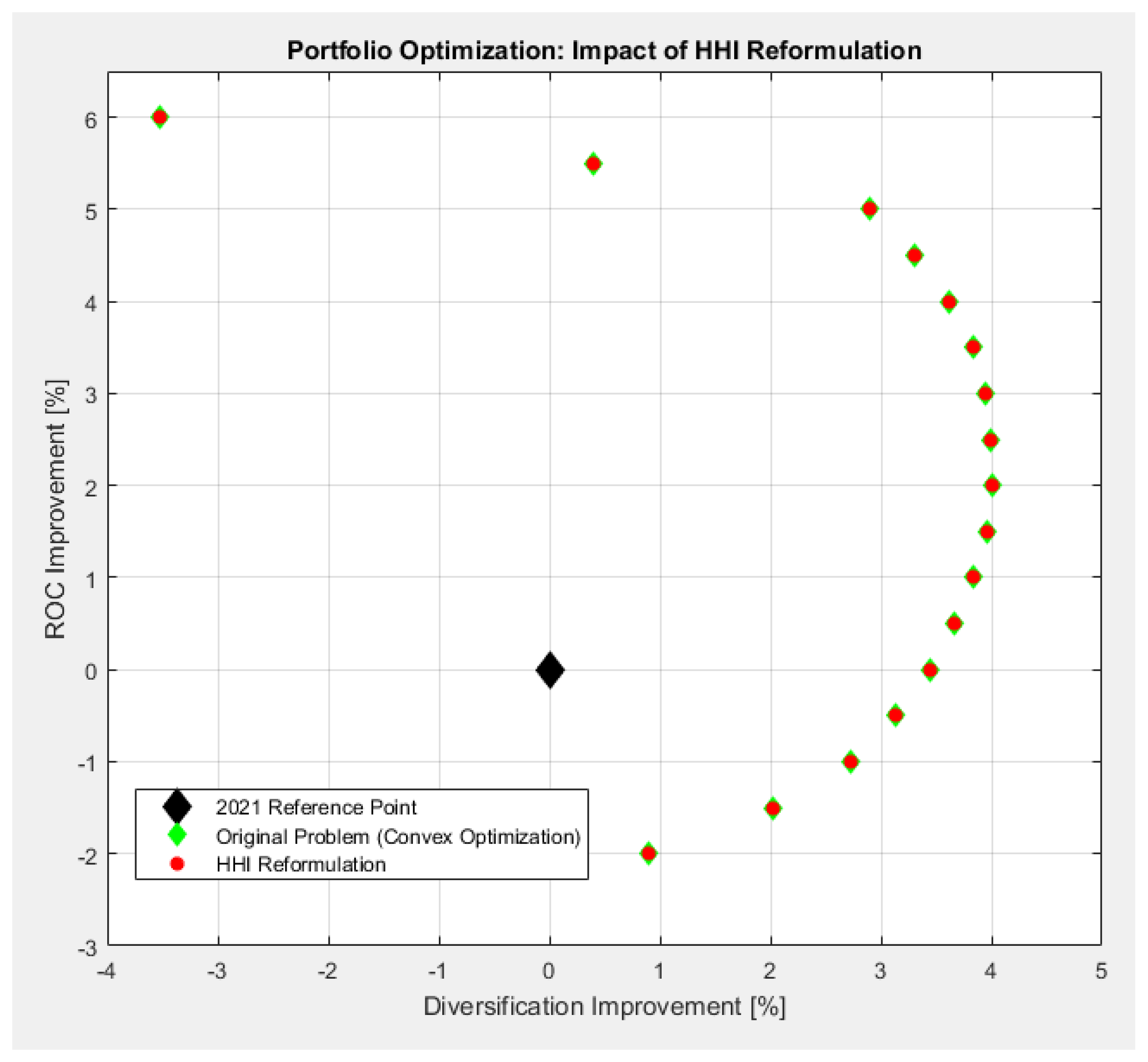
6.1. Classical Approach: Convex Optimization

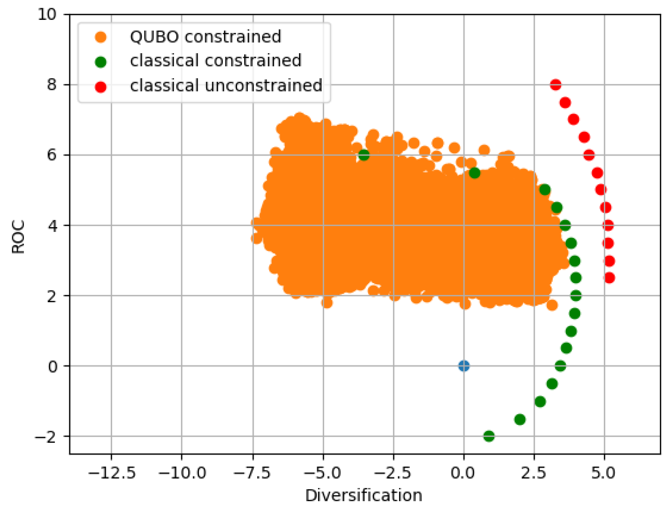
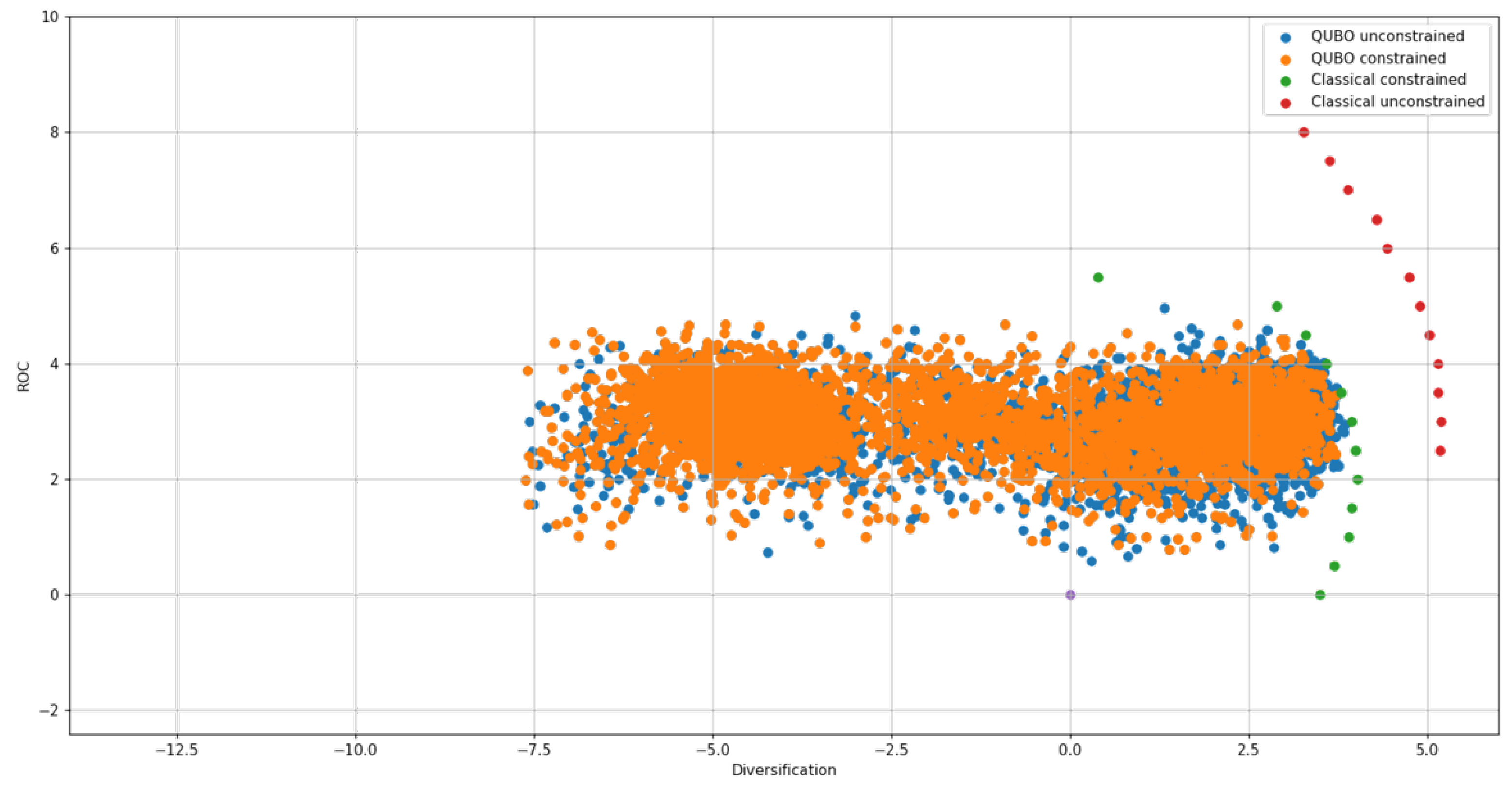
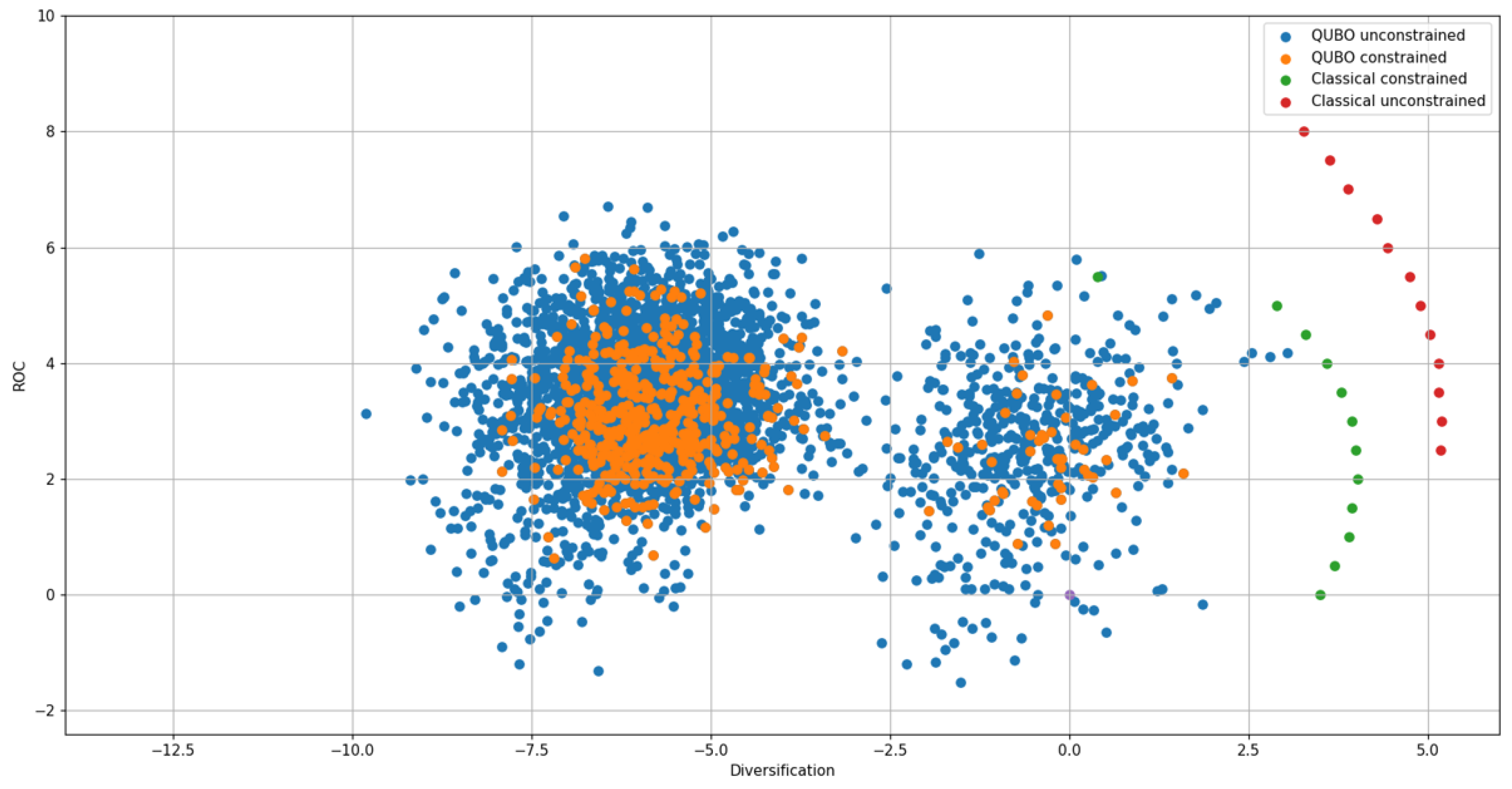
As a benchmark, we first solved our portfolio optimization problem using a classical convex optimization approach, as outlined in Section 4. To this end, all linear matrix inequality (LMI) problems were solved using the Matlab-YALMIP toolbox with the SeDuMi solver. The resulting Pareto frontier is depicted using the green diamonds in Figure 1, and is also shown using the green dots in Figure 4. Further, and for comparison, the red dots in Figure 4 visualize the Pareto frontier without the emission constraint (13).

6.2. $QUB{O}_1$ Results

Solving the QUBO problem through an annealing approach may be considered a sampling methodology. To illustrate the added value of the (quantum) annealing approach, a basic comparison with naive sampling was made. A straightforward approach was to sample from the total universe of solutions, where one of the two extreme values ($x_i=L{B}_i$ or $x_i=U{B}_i$) is the amount invested in asset i in 2030. Note that this already gave us $2^{52}$ solutions. In Figure 4, the blue and orange dots represent 18,000 random solutions, where only the one orange dot met the emission constraint. In addition, the blue dots are far from the red Pareto frontier and the orange dot is far from the green Pareto frontier.

Next, we used simulated annealing to generate solutions from the QUBO formulations, to see whether these formulations gave the desired outcomes. Simulated annealing is a classical probabilistic optimization algorithm inspired by the annealing process in metallurgy. It is used to find approximate solutions for a range of optimization and search problems. The algorithm explores the solution space by iteratively making random moves and accepting or rejecting these moves based on a probabilistic criterion. Simulated annealing is particularly effective in solving complex problems where finding an exact solution is difficult or computationally expensive. We used the implementation from D-Wave, as can be found in the python package dwave-neal (https://docs.ocean.dwavesys.com/projects/neal/en/latest/index.html (accessed on 20 March 2024)). To generate solutions, the simulated annealing approach was run 10 times for each parameter setting. For the $QUB{O}_1$ formulation, the parameters ${\lambda }_1-{\lambda }_3$ were varied in the following way. We chose ${\lambda }_3=1$ and varied ${\lambda }_1$ and ${\lambda }_2$ using the scheme ${\lambda }_i={10}^{k-4}$ for $k\in \{1,\dots ,10\}$ and $i\in \{1,2\}$.

Figure 5 shows the result of the runs described in the previous section. In comparison to the random solution of Figure 4, we see that there were many more solutions meeting the constraint (13). In addition, more solutions close to the Pareto frontier were found. However, there is room for improvement, as too few solutions with a ROC higher than 5 were obtained.

Now, when running on the real quantum annealer by D-Wave, we obtained the results depicted in Figure 6. On the real hardware, we were restricted to 100 assets, due to the number of qubits. We can see that the quantum annealer gave a broader range of solutions, compared to the simulated annealing results (for the case of similar parameters). However, of all those results, only a few lay close to the Pareto frontier and most solutions did not meet the emission constraints. Further, we can observe that the quantum annealer and simulated annealer solvers could return different sample sets, even with the same objective function.

6.3. $QUB{O}_2$ Results

Now, for the $QUB{O}_2$ formulation, the parameters ${\lambda }_1-{\lambda }_3$ were varied in the following way. We chose ${\lambda }_3=1$ and varied ${\lambda }_1={10}^{\frac{k}{8}-4.25}$ for $k\in \{0,\dots ,19\}$, ${\lambda }_2={10}^{\frac{l}{8}-4}$ for $l\in \{0,\dots ,11\}$ and ${\lambda }_4={10}^{\frac{m}{8}-11}$ for $m\in \{0,\dots ,11\}$. This resulted in the outcome as shown in Figure 2.

Comparing Figure 5 to Figure 2 makes it clear that the second QUBO formulation gave better results for our problem.

Remarkably, the results of Figure 2 show that the simulated annealing of a fine-tuned Hamiltonian could even outperform classical algorithms in some regimes. This was most likely caused by the parameter settings of the convex optimization numerical solver. Due to the higher required number of qubits, we were not able to run this on the real quantum annealer.

In Figure 7, an indication of the computational times is given. The solid lines represent the results of experiments, whereas the dotted lines are trend-lines, based on an exponential (classical methods) or linear (quantum approach) extrapolation. The simulated annealing approaches were faster than the classical YALMIP approach for the $N=52$ problem size, although for larger datasets the performance would also deteriorate exponentially. For the quantum annealing approach, its computational time will grow linearly, in expectation, as a function of problem size. Its relatively high off-set was here caused by the initial embedding that the D-Wave had to implement on its real hardware.The difference in the required computational time originated from the term addition in (26) and the corresponding weight ${\lambda }_4$ that had to be varied during the computations.

7. Conclusions and Further Research

In this study, we explored the application of quantum computing towards portfolio optimization, with a specific focus on multi-objective optimization. We discussed the classical challenges of portfolio management, including quadratic programming problems with binary decision variables, and the limitations of conventional solvers. Quantum computing is a promising alternative to overcome these challenges, by leveraging quantum annealing and a quantum approximate optimization algorithm (QAOA) to efficiently tackle complex optimization problems.

Our investigation of a real-world portfolio optimization problem in 2021, with a target set performance for 2030, highlighted the importance of balancing return on capital (ROC), concentration risk, and carbon footprint constraints. We formulated this problem as a QUBO problem, providing two distinct QUBO formulations to address different aspects of the problem. Using the simulated annealing approach, the second QUBO formulation proved to be better suited to finding solutions near the Pareto frontier. Due to current hardware restrictions, only limited results for the real quantum annealer were shown. Here, both the low number of qubits and the limited annealing time restricted us from finding better solutions for now.

Our experimental results revealed the potential of quantum computing in finding solutions that meet stringent emission constraints. Sampling from the same Hamiltonian, simulated annealing outperformed quantum annealing in terms of solutions near the Pareto frontier. This suggests that further fine-tuning of the QUBO parameters in combination with a better understanding of the solvers may yield even better outcomes. Note the QUBO approach generated multiple sample solutions, where the original approach only generated a small set of Pareto solution. This is already valuable in practice, where we unearthed a rich tapestry of solutions beyond the original optimal set, offering a wealth of valuable insights and alternative pathways worthy of exploration.

• Recommendations for further research:

• Refinement of QUBO Formulations: We recommend further refinement of the QUBO formulations to better capture the nuances of the portfolio optimization problem. Fine-tuning penalty and preference parameters, especially in the second QUBO formulation, could lead to improved results.
• Exploration of Alternative Quantum Algorithms: While quantum annealing has been shown to be promising, it might be worthwhile to explore other quantum algorithms, such as QAOA, for portfolio optimization. Comparative studies could help determine the most effective approach.
• Quantum Computing Hardware Development: As quantum computing hardware continues to advance, we recommend staying up to date with developments from leading companies like Google, IBM, and D-Wave. Newer, more powerful quantum computers may provide even better solutions for portfolio optimization.
• Integration with Traditional Portfolio Management: Quantum computing can be used in conjunction with traditional portfolio management techniques. We recommend exploring hybrid approaches that leverage the strengths of both classical and quantum computing to enhance portfolio management strategies.
• Validation on Diverse Datasets: It is crucial to validate the quantum computing solutions on diverse datasets and real-world scenarios, to ensure their robustness and practical applicability. Additionally, investigating the scalability of quantum solutions for larger portfolios is essential.
• Continuous Monitoring and Improvement: Portfolio management is an ongoing process, and quantum solutions should be continuously monitored and improved to adapt to changing market dynamics and investor preferences.

In conclusion, quantum computing holds great promise for portfolio optimization, offering more efficient and robust solutions for the financial sector. However, ongoing research and development, along with the careful consideration of formulation and hardware advancements, are essential to fully harness the potential of quantum computing in this domain.

References

1. Markowitz, H. Harry Markowitz: Selected Works; World Scientific: Singapore, 2009; Volume 1. [Google Scholar]
2. Radulescu, M.; Radulescu, C.Z. A Multi-objective Approach to Multi-period: Portfolio Optimization with Transaction Costs. In Financial Decision Aid Using Multiple Criteria; Springer: Cham, Switzerland, 2018; pp. 93–112. [Google Scholar]
3. Xidonas, P.; Mavrotas, G.; Hassapis, C.; Zopounidis, C. Robust multiobjective portfolio optimization: A minimax regret approach. Eur. J. Oper. Res. 2017, 262, 299–305. [Google Scholar] [CrossRef]
4. Skaf, J.; Boyd, S. Multi-Period Portfolio Optimization with Constraints and Transaction Costs. Working Manuscript. 2009. Available online: https://web.stanford.edu/~boyd/papers/pdf/dyn_port_opt.pdf (accessed on 20 March 2024).
5. Liagkouras, K.; Metaxiotis, K. Multi-period mean–variance fuzzy portfolio optimization model with transaction costs. Eng. Appl. Artif. Intell. 2018, 67, 260–269. [Google Scholar] [CrossRef]
6. Fulga, C.; Stanojević, B. Single period portfolio optimization with fuzzy transaction costs. In Proceedings of the 20th International Conference EURO Mini Conference “Continuous Optimization and Knowledge-Based Technologies”, EurOPT 2008, Neringa, Lithuania, 20–23 May 2008; Vilnius Gediminas Technical University: Vilnius, Lithuania, 2008. [Google Scholar]
7. Pang, T.; Hussain, A. A stochastic portfolio optimization model with complete memory. Stoch. Anal. Appl. 2017, 35, 742–766. [Google Scholar] [CrossRef]
8. Pang, T.; Varga, K. Portfolio Optimization for Assets with Stochastic Yields and Stochastic Volatility. J. Optim. Theory Appl. 2019, 182, 691–729. [Google Scholar] [CrossRef]
9. Del Pia, A.; Dey, S.S.; Molinaro, M. Mixed-integer quadratic programming is in NP. Math. Program. 2017, 162, 225–240. [Google Scholar]
10. Garey, M.R.; Johnson, D.S. Computers and Intractability; Freeman: San Francisco, CA, USA, 1979; Volume 174. [Google Scholar]
11. Li, D.; Sun, X.; Gu, S.; Gao, J.; Liu, C. Polynomially solvable cases of binary quadratic programs. In Optimization and Optimal Control; Springer: New York, NY, USA, 2010; pp. 199–225. [Google Scholar]
12. Poli, R.; Kennedy, J.; Blackwell, T. Particle swarm optimization: An overview. Swarm Intell. 2007, 1, 33–57. [Google Scholar] [CrossRef]
13. Grefenstette, J.J. Genetic algorithms and machine learning. In Proceedings of the Sixth Annual Conference on Computational Learning Theory, Santa Cruz, CA, USA, 26–28 July 1993; pp. 3–4. [Google Scholar]
14. Angus, D.; Woodward, C. Multiple objective ant colony optimisation. Swarm Intell. 2009, 3, 69–85. [Google Scholar] [CrossRef]
15. Kirkpatrick, S.; Gelatt, C.D., Jr.; Vecchi, M.P. Optimization by simulated annealing. Science 1983, 220, 671–680. [Google Scholar] [CrossRef]
16. Zanjirdar, M. Overview of Portfolio Optimization Models. Adv. Math. Financ. Appl. 2020, 5, 1–16. [Google Scholar]
17. Ronagh, P.; Woods, B.; Iranmanesh, E. Solving constrained quadratic binary problems via quantum adiabatic evolution. Quantum Inf. Comput. 2016, 16, 1029–1047. [Google Scholar] [CrossRef]
18. McGeoch, C.C. Adiabatic quantum computation and quantum annealing: Theory and practice. Synth. Lect. Quantum Comput. 2014, 5, 1–93. [Google Scholar]
19. Farhi, E.; Harrow, A.W. Quantum supremacy through the quantum approximate optimization algorithm. arXiv 2016, arXiv:1602.07674. [Google Scholar]
20. Neumann, N.; Phillipson, F.; Versluis, R. Machine learning in the quantum era. Digit. Welt 2019, 3, 24–29. [Google Scholar] [CrossRef]
21. Möller, M.; Vuik, C. On the impact of quantum computing technology on future developments in high-performance scientific computing. Ethics Inf. Technol. 2017, 19, 253–269. [Google Scholar] [CrossRef]
22. Gemeinhardt, F.G. Quantum Computing: A Foresight on Applications, Impacts and Opportunities of Strategic Relevance. Ph.D. Thesis, Universität Linz, Linz, Austria, 2020. [Google Scholar]
23. Resch, S.; Karpuzcu, U.R. Quantum computing: An overview across the system stack. arXiv 2019, arXiv:1905.07240. [Google Scholar]
24. Piattini, M.; Peterssen, G.; Pérez-Castillo, R.; Oliver, J.L.H.; Serrano, M.A.; González, G.J.H.; de Guzmán, I.G.R.; Paradela, C.A.; Polo, M.; Murina, E.; et al. The Talavera Manifesto for Quantum Software Engineering and Programming. In Proceedings of the QANSWER, Talavera, Spain, 12–18 February 2020; pp. 1–5. [Google Scholar]
25. Van den Brink, R.; Phillipson, F.; Neumann, N.M. Vision on next level quantum software tooling. In Proceedings of the Computation Tools, Venice, Italy, 5–9 May 2019. [Google Scholar]
26. Neumann, N.M.P.; van der Schoot, W.; Sijpesteijn, T. Quantum Cloud Computing from a User Perspective. In Proceedings of the International Conference on Innovations for Community Services, Bamberg, Germany, 11–13 September 2023; Springer: Cham, Switzerland, 2023; pp. 236–249. [Google Scholar]
27. Orus, R.; Mugel, S.; Lizaso, E. Quantum computing for finance: Overview and prospects. Rev. Phys. 2019, 4, 100028. [Google Scholar] [CrossRef]
28. Elsokkary, N.; Khan, F.S.; La Torre, D.; Humble, T.S.; Gottlieb, J. Financial Portfolio Management Using D-Wave Quantum Optimizer: The Case of Abu Dhabi Securities Exchange; Technical report; Oak Ridge National Lab. (ORNL): Oak Ridge, TN, USA, 2017. [Google Scholar]
29. Venturelli, D.; Kondratyev, A. Reverse quantum annealing approach to portfolio optimization problems. Quantum Mach. Intell. 2019, 1, 17–30. [Google Scholar] [CrossRef]
30. Marzec, M. Portfolio optimization: Applications in quantum computing. In Handbook of High-Frequency Trading and Modeling in Finance; Wiley: Hoboken, NJ, USA, 2016; pp. 73–106. [Google Scholar]
31. Cohen, J.; Khan, A.; Alexander, C. Portfolio Optimization of 40 Stocks Using the D-Wave Quantum Annealer. arXiv 2020, arXiv:2007.01430. [Google Scholar]
32. Cohen, J.; Khan, A.; Alexander, C. Portfolio Optimization of 60 Stocks Using Classical and Quantum Algorithms. arXiv 2020, arXiv:2007.08669. [Google Scholar]
33. Kaushik, N.; Raj, A.; Srivastava, M.; Ansari, M.S.; Pushpalatha, M.; Gayathri, M.; Kavisankar, L.; Deshpande, S.; Venkatraman, R. Financial Portfolio Optimization: A QAOA and VQE Formulation for Sharpe Ratio Maximization. In Proceedings of the 2023 6th International Conference on Recent Trends in Advance Computing (ICRTAC), Chennai, India, 14–15 December 2023; IEEE: Piscataway, NJ, USA, 2023; pp. 575–581. [Google Scholar]
34. Phillipson, F.; Bhatia, H.S. Portfolio optimisation using the D-Wave quantum annealer. In Proceedings of the International Conference on Computational Science, Krakow, Poland, 16–18 June 2021; Springer: Cham, Switzerland, 2021; pp. 45–59. [Google Scholar]
35. Sakuler, W.; Oberreuter, J.M.; Aiolfi, R.; Asproni, L.; Roman, B.; Schiefer, J. A real world test of Portfolio Optimizationwith Quantum Annealing. arXiv 2024, arXiv:2303.12601. [Google Scholar]
36. George, B.; Loo, J.; Jie, W. Novel multi-objective optimisation for maintenance activities of floating production storage and offloading facilities. Appl. Ocean. Res. 2023, 130, 103440. [Google Scholar] [CrossRef]
37. Afshari, H.; Tosarkani, B.M.; Jaber, M.Y.; Searcy, C. The effect of environmental and social value objectives on optimal design in industrial energy symbiosis: A multi-objective approach. Resour. Conserv. Recycl. 2020, 158, 104825. [Google Scholar] [CrossRef]
38. Lucas, A. Ising formulations of many NP problems. Front. Phys. 2014, 2, 5. [Google Scholar] [CrossRef]
39. Glover, F.; Kochenberger, G.; Hennig, R.; Du, Y. Quantum Bridge Analytics I: A tutorial on formulating and using QUBO models. Ann. Oper. Res. 2019, 17, 335–371. [Google Scholar] [CrossRef]
40. Domino, K.; Koniorczyk, M.; Krawiec, K.; Jałowiecki, K.; Deffner, S.; Gardas, B. Quantum annealing in the NISQ era: Railway conflict management. Entropy 2023, 25, 191. [Google Scholar] [CrossRef]
41. Neukart, F.; Compostella, G.; Seidel, C.; Von Dollen, D.; Yarkoni, S.; Parney, B. Traffic flow optimization using a quantum annealer. Front. ICT 2017, 4, 29. [Google Scholar] [CrossRef]
42. Phillipson, F.; Chiscop, I. Multimodal container planning: A QUBO formulation and implementation on a quantum annealer. In Proceedings of the International Conference on Computational Science, Krakow, Poland, 16–18 June 2021; Springer: Cham, Switzerland, 2021; pp. 30–44. [Google Scholar]
43. Chiscop, I.; Nauta, J.; Veerman, B.; Phillipson, F. A hybrid solution method for the multi-service location set covering problem. In Proceedings of the Computational Science–ICCS 2020: 20th International Conference, Amsterdam, The Netherlands, 3–5 June 2020; Proceedings, Part VI 20. Springer: Berlin/Heidelberg, Germany, 2020; pp. 531–545. [Google Scholar]
44. Phillipson, F. Quantum Computing in Telecommunication—A Survey. Mathematics 2023, 11, 3423. [Google Scholar] [CrossRef]
45. Lin, M.M.; Shu, Y.C.; Lu, B.Z.; Fang, P.S. Nurse Scheduling Problem via PyQUBO. arXiv 2023, arXiv:2302.09459. [Google Scholar]
46. Nazareth, D.P.; Spaans, J.D. First application of quantum annealing to IMRT beamlet intensity optimization. Phys. Med. Biol. 2015, 60, 4137. [Google Scholar] [CrossRef]
47. Rhoades, S.A. The Herfindahl-Hirschman Index. Fed. Res. Bull. 1993, 79, 188. [Google Scholar]
48. Lobo, M.; Fazel, M.; Boyd, S. Portfolio Optimization with Linear and Fixed Transaction Costs. Ann. Oper. Res. 2007, 152, 341–365. [Google Scholar] [CrossRef]
49. Boyd, S.; Busseti, E.; Diamond, S.; Kahn, R.N.; Kwangmoo, K.; Nystrup, P.; Speth, J. Multi-Period Trading via Convex Optimization. Found. Trends Optim. 2017, 3, 1–76. [Google Scholar] [CrossRef]
50. Boyd, S.; El Ghaoui, L.; Feron, E.; Venkataramanan, B. Linear Matrix Inequalities in System and Control Theory; Soc. for Industrial and Applied Mathematics (SIAM): Philadelphia, PA, USA, 1994. [Google Scholar]
51. Boyd, S.; Vandenberghe, L. Convex Optimization; Cambridge University Press: Cambridge, UK, 2004. [Google Scholar]
52. Nesterov, Y.; Nemirovskii, A. Interior-Point Polynomial Methods in Convex Programming; Soc. for Industrial and Applied Mathematics (SIAM): Philadelphia, PA, USA, 1994. [Google Scholar]
53. Sturm, J.F. Using SeDuMi 1.02, a Matlab Toolbox for Optimization over Symmetric Cones. Optim. Methods Softw. 1999, 11–12, 625–653. [Google Scholar] [CrossRef]
Figure 1. The classical solution frontier with the reformulation (17) of the HHI (red) is virtually identical to the solution frontier of the problem with the original (7) objective (green).
Mathematics 12 01291 g001
Figure 2. Simulated annealing for Q U B O 2 (26) yielded points that reconstruct the upper half of the Pareto frontier.
Mathematics 12 01291 g002
Figure 3. The approximate inverse G C inv (32) in blue versus the true inverse of the capital growth factor G C (31) in green.
Mathematics 12 01291 g003
Figure 4. Random sampling of 18,000 portfolios yielded only one portfolio (orange) that met the emission constraint. Furthermore, all sampled portfolios lay far from their respective Pareto frontiers.
Mathematics 12 01291 g004
Figure 5. Simulated annealing of Q U B O 1 (18) yielded many more portfolios meeting the emission constraint in comparison to random sampling. Furthermore, their risk and return characteristics reconstructed a small section of the green Pareto frontier, which was the optimal solution for the problem with the emission constraint.
Mathematics 12 01291 g005
Figure 6. Quantum annealing of Q U B O 1 found more portfolios meeting the emission constraints than random sampling, but not as many as simulated annealing. Furthermore, the obtained portfolios were concentrated within two clusters clearly separated from the (green) Pareto frontier.
Mathematics 12 01291 g006
Figure 7. The computation times to solve the problems as a function of the number of assets in the portfolio. The solid lines are the results of experiments, the dotted lines are trend-lines, based on an exponential extrapolation for the classical methods and linear extrapolation for the quantum approach.
Mathematics 12 01291 g007