Intelligent Low-Consumption Optimization Strategies: Economic Operation of Hydropower Stations Based on Improved LSTM and Random Forest Machine Learning Algorithm

Abstract

The economic operation of hydropower stations has the potential to increase water use efficiency. However, there are some challenges, such as the fixed and unchangeable flow characteristic curve of the hydraulic turbines, and the large number of variables in optimal load distribution, which limit the progress of research. In this paper, we propose a new optimal method of the economic operation of hydropower stations based on improved Long Short-Term Memory neural network (I-LSTM) and Random Forest (RF) algorithm. Firstly, in order to accurately estimate the water consumption, the LSTM model’s hyperparameters are optimized using improved particle swarm optimization, and the I-LSTM method is proposed to fit the flow characteristic curve of the hydraulic turbines. Secondly, the Random Forest machine learning algorithm is introduced to establish a load-distribution model with its powerful feature extraction and learning ability. To improve the accuracy of the load-distribution model, we use the K-means algorithm to cluster the historical data and optimize the parameters of the Random Forest model. A Hydropower Station in China is selected for a case study. It is shown that (1) the I-LSTM method fits the operating characteristics under various working conditions and actual operating characteristics of hydraulic turbines, ensuring that they are closest to the actual operating state; (2) the I-LSTM method is compared with Support Vector Machine (SVM), Extreme Learning Machine (ELM) and Long Short-Term Memory neural network (LSTM). The prediction results of SVM have a large error, but compared with ELM and LSTM, MSE is reduced by about 46% and 38% respectively. MAE is reduced by about 25% and 21%, respectively. RMSE is reduced by about 27% and 24%, respectively; (3) the RF algorithm performs better than the traditional dynamic programming algorithm in load distribution. With the passage of time and the increase in training samples, the prediction accuracy of the Random Forest model has steadily improved, which helps to achieve optimal operation of the units, reducing their average total water consumption by 1.24%. This study provides strong support for the application of intelligent low-consumption optimization strategies in hydropower fields, which can bring higher economic benefits and resource savings to renewable energy production.

1. Introduction

Energy plays a key role in the development of a country and the improvement of people’s living standards. The increasing demand for energy is rapidly depleting traditional energy sources [1,2]. Consequently, in recent years, the focus of power generation has shifted towards renewable energy [3]. Among all available renewable sources, hydropower stands out as a clean, efficient and easily utilizable power-generation technology [4,5]. Efficient and economical operation of hydropower can bring economic benefits and resource savings to hydropower stations [6]. The general objective of economic operation within a hydropower station is to adjust the start–stop status and output of each unit under a given load curve, identify the optimal combination of unit operations, achieve optimal internal load distribution and maximize the economic efficiency of the hydropower station to meet the requirements of safe, high-quality and economical operation [7,8,9].

The economic operation of hydropower stations involves two stages: fitting the flow characteristic curve of the hydraulic turbines [10] and load distribution [11]. It firstly needs to calculate the corresponding unit’s output at the current head and flow, or the corresponding unit’s water consumption at the current head and output according to the flow characteristic curve of the unit, and then it can proceed to the unit load distribution. This initial step is vital to the entire process of economic operation within the hydropower station and is a key factor influencing the results of unit load distribution [12,13,14]. Skjelbred et al. [15] studied spline nonlinear interpolation of hydraulic turbine efficiency curves, and demonstrated good performance in day-ahead scheduling at hydropower stations. Wu Q et al. [16] used radial basis function neural networks to expand and fit the characteristics of hydraulic turbines, finding that an increased number of learning samples significantly improves the accuracy and reliability of the fitting. Liu D et al. [17] proposed a method to adjust the hydraulic turbine model using input–output parameters, offering certain reliability. Li J et al. [18] converted the nonlinear characteristics of hydraulic turbines into torque and flow characteristics based on neural networks, suitable for real-time simulation. Li J et al. [19] conducted real-time simulation directly based on a BP neural network to solve the problem that it is difficult to fit the comprehensive characteristic curve of hydraulic turbine during the large fluctuation transition process of hydropower units. Xu L et al. [10] applied the MEA-BP neural network with the ability of nonlinear approximation to fit the operating characteristic curve of hydraulic turbines effectively, and the fitting accuracy was better than that of the traditional BP method.

These methods used different machine learning methods to fit the flow characteristic curve of hydraulic turbines, and achieved varying degrees of effectiveness. However, current machine learning methods are mostly shallow learning methods [20,21], and deep learning methods are rarely applied, failing to fully explore the performance advantages of deep learning in adaptive feature extraction and learning ability [22,23,24]. In addition, the flow characteristic curve of the hydraulic turbines is mostly generated based on model curve conversion or actual operation data fitting during the initial production stage. Once it is put into the economic operation model in the plant, it does not consider coordinated adjustment with the operating status of the unit. For example, it does not consider the possible changes in the flow characteristic curve after each unit maintenance.

Regarding the load distribution of hydropower units, scholars both domestically and internationally have undertaken extensive research. For instance, Alvarez G E [25] introduced a new mixed-integer linear programming model that quickly and conveniently determines unit combinations, effectively reducing computation time. Oluwatosin O et al. [26] proposed a data-driven Artificial Neural Network (ANN) model coupled with a novel Composite Pareto Multi-Objective Differential Evolution (CPMDE) for hydrological simulation and multi-objective numerical optimization in hydropower production. Amani A et al. [27] applied Sequential Mixed-Integer Linear Programming (MLP) to address specific optimization challenges in hydropower systems and verified its effectiveness. Paredes M et al. [28] approximated the daily ahead unit combination problem of hydropower units using continuous convex semidefinite programming relaxation.

In general, the current methods of load allocation mainly include traditional algorithms such as Lagrangian relaxation (LR) [29] and dynamic programming (DP) [30], as well as a variety of intelligent optimization algorithms such as particle swarm optimization (PSO) [31], genetic algorithm (GA) [32] and bat algorithm (BA) [33]. However, as hydropower stations continue to expand and the number of units increases, dynamic programming algorithms encounter a ‘dimensionality explosion’, leading to exponentially increasing computational complexity. Most other intelligent optimization algorithms are based on physically driven models, which are difficult to modify once the model and algorithm are established. Also, they often overlook the significance of historical data and decisions. Once a model and algorithm are set, their computational efficiency and solution accuracy do not change. But machine learning methods, with their strong feature extraction and learning capabilities, are worth exploring for unit load-distribution problems [34]. Based on the above theory, the research in this paper is as follows:

(a)

In view of the low precision of traditional curve fitting methods and the difficulty in determining mathematical formulas, based on the large amount of real machine characteristic parameter data (water head, flow, output) generated during the actual operation of the unit, and combined with the hydraulic turbine model test data, the improved particle swarm optimization algorithm is used to optimize the hyperparameters of the deep long-short term memory network to determine the network model. An improved Long Short-Term Memory neural network (I-LSTM) algorithm for fitting the flow characteristics curve of a hydraulic turbine is proposed.

(b)

We use the Random Forest (RF) algorithm of machine learning to perform load distribution for hydropower units. This machine learning method can train massive amounts of historical decision data, build mapping relationships between inputs and outputs, and continuously revise them over time. Solving the load-distribution problem of hydropower units to verify the effectiveness and accuracy of the algorithm.

The rest of the paper is outlined as follows: Section 2 introduces the hydraulic turbine flow characteristic curve model based on the I-LSTM algorithm and the related parameter-optimization method. Section 3 introduces the related theory of the load-distribution model of Random Forest algorithm. Section 4 analyzes and discusses the actual case. Finally, the conclusions to this study are summarized in Section 5.

2. Introduction Hydraulic Turbine Flow Characteristic Curve Fitting Based on I-LSTM

The flow characteristic curves of hydraulic turbines are usually obtained from model tests when they are put into operation, which cannot reflect the dynamic influence of installation, maintenance, operation and other factors on the unit state in time. Therefore, with the model based on model experimental data, it is difficult to accurately reflect the flow characteristics under various actual operating conditions with time. Thus, this paper synthetically uses model test data, historical operation data and real-time operation data to fit the flow characteristic curve of hydraulic turbines. However, the current commonly used curve fitting methods, such as the least square method [35] and polynomial fitting, cannot effectively use a large number of historical data of real machine operation, and cannot give full play to the full value of real machine operation data.

This paper proposes an enhanced method for fitting unit flow characteristic curves based on an improved LSTM approach. The learning model’s training data consists of the model test data from unit commissioning and actual operational data. This approach not only considers the full-head operating conditions of the unit but also comprehensively incorporates the high-efficiency operating zone in the actual operation process. This effectively addresses the accuracy and precision issues in training networks that stem from relying on a single data source. This method offers a precise model for predicting unit output, crucial for optimizing hydropower unit combinations and load distribution, thereby improving decision-making accuracy in unit load management.

2.1. Hydraulic Turbine Flow Characteristic Curve Fitting Model

Long Short-Term Memory networks (LSTM) [36] were introduced to overcome the rapidly vanishing gradient problem encountered in training Recurrent Neural Networks (RNN) with gradient descent methods. This phenomenon occurs during the backward propagation of gradients along the sequence. As shown in Figure 1, the LSTM cell contains three gates: input gate, forget gate and output gate [37]. $c_{t-1}$ is cellular memory at time t − 1, $c_t$ is cellular memory at time t, $h_{t-1}$ is hidden layer information at time t − 1, $h_t$ is hidden layer information at time t, $x_t$ is input at time t, $i_t$ is input gate output, $f_t$ is forget gate output, $o_t$ is output gate output, ${\tilde{c}}_t$ is candidate value vector, $\sigma$ and $\tanh$ are activation functions and $W_{xf}$, $W_{xi}$, $W_{xc}$, $W_{xo}$ represent corresponding weight factor matrices.

To better unearth the hidden relationships between various characteristic parameters of hydraulic turbines, deep neural network models are utilized for data feature extraction. The overall structure of the model is divided into three main parts: input layer, hidden layers and output layer. Given that the input data feature both water head and output, the network’s input layer is set as a two-dimensional fully connected layer (FC), with training set data $X_i\left(H_i,P_i\right)$ of length T. After normalization, the data are fed into the hidden layers; there are two LSTM layers in the hidden layers, each containing multiple memory units. To prevent model overfitting, a dropout layer is added after each LSTM layer. The data then pass through denormalization before being output from the output layer. Since the output data are the flow, the output layer is set as a one-dimensional fully connected layer, producing the model’s predicted value Y. Apart from data exchange between neurons within the LSTM layers, neurons in other layers are independent of each other, with information exchange occurring only between layers.

2.2. Data Preprocessing

The collected data include both model experiments and the actual operation of the units. The model experiments cover full-head efficiency tests, which allow the calculation of unit water consumption based on the current unit head and efficiency. Actual operational data include head, flow and output, constituting time-series data. To eliminate the impact of different units of measurement across parameters, it is essential to normalize the data, ensuring comparability between various data indicators. This study uses the min-max normalization method, as outlined in Equation (1).

$$x_{norm,i}=\frac{x_i-X_{\min }}{X_{\max }-X_{\min }}$$

(1)

where $x_i$ is the i-th sample data; $X_{\min }, X_{\max }$ are the minimum and maximum values of dataset X in each dimension, respectively; $x_{norm,i}$ is the i-th sample after normalization.

After normalization, the dataset is divided into training, validation and test sets. The total dataset comprises 3000 data points, with the training set accounting for 90% of the total, the test set 10% and the validation set 20% of the training set. Following this division, hyperparameters of the established network model are optimized based on the segregated datasets.

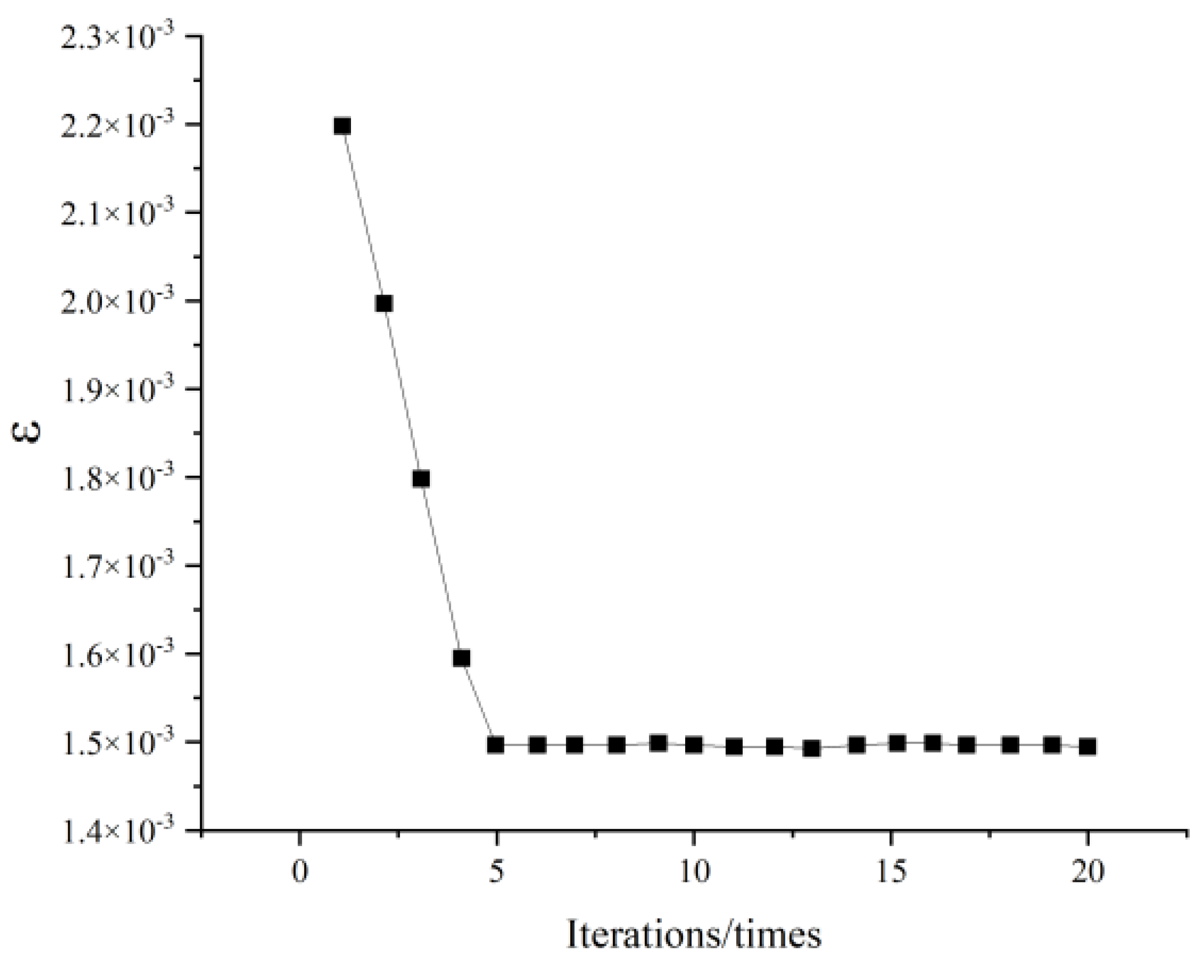
2.3. Optimization of Model Parameters

The capacity of a neural network to fit data is directly determined by the number of neurons and layers in its hidden layers, while the learning rate and iteration count influence the training process and outcome. An Improved Particle Swarm Optimization (IPSO) algorithm is used to determine the optimal number of neurons, learning rate and iteration count in the hidden layers, thereby optimizing the network model’s parameters.

A nonlinear variable weight is introduced to enhance the optimization capability and speed of the Particle Swarm Optimization (PSO) algorithm [38]. The variation of the weight parameter ($w$) is detailed in Equation (2).

$$w=w_{\max }-(w_{\max }-w_{\min })\cdot \arcsin (\frac{t}{t_{\max }}\cdot \frac{2}{\pi })$$

(2)

where $w_{\max }$ and $w_{\min }$ are the maximum and minimum values of $w$; t is the current iteration number; and $t_{\max }$ is the maximum iteration number.

At the beginning of particle swarm optimization, t is small, $w$ is close to the maximum and $w$ decreases slowly. This slow decrease ensures the algorithm’s global optimization ability. As t increases, $w$ decreases nonlinearly with an increasing range, enhancing the algorithm’s local optimization ability and flexibility.

In order to reflect the changes of the PSO algorithm before and after improvement, the test functions of Equations (3) and (4) are used to test it.

$$fitness=e^{(\cos (2\pi \cdot x_1)+\cos (2\pi \cdot x_2))/2}-3$$

(3)

$$fitness=\frac{\sin (\sqrt{x_1^2+x_2^2})}{\sqrt{x_1^2+x_2^2}}+e^{(\cos (2\pi \cdot x_1)+\cos (2\pi \cdot x_2))/2}-3$$

(4)

When $x_1=x_2=0$, use Equation (3) to calculate the fitness value. When $x_1$ and $x_2$ are not 0, use Equation (4) to calculate the fitness value. The parameters related to IPSO and PSO are the following: the weights of IPSO are $w_{\max }=0.9$, $w_{\min }=0.1$, the weight $w$ of PSO is 0.6 and the other parameters are consistent. After several calculations, take the mean value; the final result is shown in Figure 2.

It is obvious from Figure 2 that IPSO can reach the optimal value in about 10 steps, while PSO can reach the optimal value in about 20 steps, and the optimization speed has been significantly improved.

The number of neurons in the first and second hidden layers $(h_1,h_2)$, the model learning rate $(\epsilon )$ and the number of training times $\left(ep\right)$ are among the important parameters in the constructed network model. The dimensionality of the particle’s search solution space is set to four dimensions. The value of adaptation for the i-th particle is computed using the formula in Equation (5).

$$fi{t}_i=\frac{1}{n}{\displaystyle \sum _{j=1}^n}{({\widehat{y}}_t^j-y_t^j)}^2$$

(5)

where $fi{t}_i$ is the fitness value of the i-th particle; n is the number of samples in the test set. ${\widehat{y}}_t^j$ and $y_t^j$ are the predicted value and the labeled value of the network parameter for the j-th sample of the corresponding model of particle i, respectively, and the predicted value is computed based on the parameter information carried by the particles after the training of the network model.

As illustrated in Figure 3, the steps for optimizing neural network parameters with IPSO are as follows:

(1)

Initialize individual parameters, including population size, iteration count, learning factors and the range of particle velocity and position values.

(2)

Initialize particle position and velocity information, randomly generating a certain number of population particles $X_{i,0}(h_1,h_2,\epsilon ,ep),i=1,2,\dots ,n$, with each dimension value within the defined range.

(3)

Calculate the fitness value for each particle $X_i$ based on the established objective function, determine the global and individual extrema of the initial population and record each particle’s best position as its historical optimum.

(4)

In each iteration, update the velocity and position information of the particles, calculate the fitness values for the new population and determine the individual and global extrema for the current population.

(5)

Repeat steps (3)–(4) until the maximum number of iterations or desired accuracy is achieved, output the optimal network parameters and train the network model.

Figure 3. Flow chart of IPSO optimization of network parameters.

Figure 3. Flow chart of IPSO optimization of network parameters.

3. Load Distribution of Hydropower Units Based on Random Forest Algorithm

3.1. Data Preprocessing Based on K-Means Clustering Algorithm

It is simple to discover that there is some temporal repetitiveness in the unit load-distribution historical decision data gathered for this research. Thus, this article first uses the K-means method to cluster the historical data in order to completely uncover the regularity of the unit load-distribution historical decision data on the longer scale and improve the forecast accuracy of the machine learning model.

With the benefits of simplicity and speed, the K-means algorithm is a popular unsupervised learning technique that can automatically categorize data based on their attributes [39]. The method groups comparable data into a single category and accomplishes the goal of grouping data by calculating the degree of correlation between two pieces of data using Euclidean distance. The K-means clustering algorithm’s particular stages are as follows:

(1)

For a set of datasets, $D=\left\{M_1,M_2,\dots ,M_n\right\},M=\left(X,Y\right)$. First, K values are randomly selected as the initial clustering centers $c=\left\{c_1,c_2,\dots c_K\right\}$.

(2)

The Euclidean distance of each sample to a cluster center is calculated, and it is classified into one category with the nearest cluster center to form K categories.

(3)

The average clustering centers of the K classes are recalculated, and the original clustering centers are replaced with new ones.

(4)

Repeat steps (2) and (3), and stop when you know that there is no change or no change in the cluster center c.

The choice of clustering categories K has a relatively obvious impact on the clustering effect. It is vital to ascertain the number of clustering centers since the impact of these centers on the clustering effect is rather evident. The method used in this paper, as indicated by Equation (6), is to find the sum of the squared values of the distance difference for each sample and clustering center for each case within a given range of clustering centers. Based on the relationship between the total error and the number of clustering centers, a reasonable number of clusters are then selected.

Error sum of squares formula:

$$SSE={\displaystyle \sum _{n=1}^N{\displaystyle \sum _{k=1}^K{(D_k-c_k)}^2}}$$

(6)

where SSE is the total error of n classes and N is the upper bound of the clustering centers seeking value.

After determining the number of cluster centers, cluster analysis is performed on the collected data. The basic idea is that, according to the input form of the training data of the machine learning model, the collected data take the unit water head and external load as a sample, and then cluster.

3.2. Modelling of Unit Load Distribution Based on RF

The main goal of the Random Forest algorithm is to solve the overfitting issue with a single decision tree by randomly selecting a new subset of training data from the original training set, building multiple decision trees using this new subset, and then combining the learning from each decision tree to yield the most accurate prediction.

The structure of the model built for solving the unit load distribution using the Random Forest algorithm is shown in Figure 4. Where D is all the training set samples, X and Y are the input and output quantities, respectively, $D_1$ to $D_n$ is the sub-training set, $\left\{t{r}_i,i=1,2,\dots ,k\right\}$ is the k decision trees established and y is the final prediction value.

The unit load-distribution model based on Random Forest is solved via the following three main steps:

• Model building

Let the original training dataset D have M samples, the total number of features be S and the number of decision trees to be built be k.

(1)

Extraction of sub-training set: M samples are randomly selected from the dataset D using the Bootstrap method to form S sub-training datasets and construct M decision trees, and the samples that are not selected form M out-of-bag data.

(2)

Build decision tree: randomly select F features (F ≤ M) from S features at each node of the decision tree as the segmentation feature set of the node, select the optimal segmentation feature and the optimal segmentation point using certain criteria, divide the current node into two sub-nodes and divide the training set data into these two sub-nodes as well. The segmentation process is repeated until the requirements are met.

(3)

Build a Random Forest: repeat step (2) until all k decision trees are generated and combined into a Random Forest $\left\{t{r}_i,i=1,2,\dots ,k\right\}$.

2.

Data collection and preprocessing

The data are the characteristic parameters of a hydropower station in China, including the generating head of the unit, the external load at the same time and the output of each unit at the current time. Real machine operating data are collected over a period of one year, ten days per month and ninety-six collecting instances per day. Normalization is necessary for the obtained operation data because the varying magnitudes of each parameter could cause significant gaps between the dataset’s dimensions.

3.

Model training and prediction

After the preprocessing is finished, the data are fed into Python and a Random Forest model is constructed using the Scikit-Learn module. After being proportionately split into a training and test set at random, the dataset is trained. k decision trees are used in the Random Forest to predict the test set dataset $D_t$ and obtain k predictions $\left\{y_1,y_2,\dots ,y_k\right\}$. Based on the Bagging method, the prediction results are integrated to obtain the final prediction results. In order to prevent overfitting, Random Forest can be subjected to pruning.

4. Example Analysis

4.1. Hydraulic Turbine Flow Characteristic Curve Fitting

The study focuses on a hydropower station in China, which comprises six units. The rated output of each unit is 442 MW with a rated hydraulic head of 246 m, a maximum hydraulic head of 282.6 m, a rated flow rate of 194.8 ${\mathrm{m}}^3/\mathrm{s}$ and a maximum efficiency of 96.29%.

(1)

Model Parameter Optimization

Utilizing the advantage of deep networks in data feature extraction, a deep neural network model for fitting the characteristic curves of hydraulic turbines was constructed, and the hyperparameters of the network model were optimized. The optimization parameters are set as follows: the input layer has two neurons, the output layer has one neuron and the Adam algorithm is used to train the internal parameters of LSTM units with initialization via the Xavier method. The parameters for the Improved Particle Swarm Optimization (IPSO) algorithm are set as follows: population size of 5, iteration time of 20, learning factors for particles set at $c_1=c_2=2$. The range of parameters in each dimension of a particle $X_{i,0}(n_1,n_2,\epsilon ,h)$ are [1, 100], [1, 100], [0.0001, 0.01] and [300, 600], respectively, with particle velocity ranges of [−5, 5], [−5, 5], [−0.0005, 0.0005], and [−10, 10]. In IPSO, $w_{\max }=0.9, w_{\min }=0.1$; in PSO, $w=0.5$.

The results are shown in Figure 5. The results of PSO and IPSO are obtained by averaging 10 computations each. The IPSO method is used to optimize the number of neurons in each hidden layer, the network learning rate and the number of training iterations, with the algorithm settings being the same as before. The changes in the number of neurons in each hidden layer of the LSTM network model are shown in Figure 6. As can be seen from the figure, the number of neurons in the first hidden layer $h_1$ finally stabilizes at 40, and the number of neurons in the second hidden layer $h_2$ stabilizes at 32.

Figure 7 shows the variation in the network learning rate $\epsilon$ with the number of iterations, which eventually stabilizes at 0.0015. Figure 8 reflects the change in $ep$ in the number of LSTM network training iterations with the number of IPSO iterations, with the final value stabilizing at 342. Based on the results of hyperparameter optimization, i.e., $h_1=40, h_2=32, \epsilon =0.0015, ep=342$, the network structure is determined and the LSTM network is used to train the divided training dataset.

(2)

Model Training and Prediction

In order to accelerate the speed of network training and improve efficiency, the software environment for neural network training is as follows: the programming language is Python 3.7, the programming platform is PyCharm 2021.2, the version of TensorFlow and tensorflow-gpu libraries is 2.4.0 and the Keras libraries of the TensorFlow framework are used for model building; the hardware environment is as follows: the GPU model is NNIDIA GeForce RTX 3070, and the CPU model is Intel(R) Core(TM) i7-780000. The environment is as follows: GPU model is NNIDIA GeForce RTX 3070; the CPU model is Intel(R) Core(TM) i7-7800X CPU.

Table 1. Network structure.

Network Layers (Types)	Output Dimension
dense1 (FC)	2
lstm1 (LSTM)	$h_1$
dropout1 (Dropout)	$h_1$
lstm2 (LSTM)	$h_2$
dropout2 (Dropout)	$h_2$
dense2 (FC)	1

displays the output dimensions for each layer of the network as well as the network topology that was built in the article. The Dropout technique is used between the two LSTM network layers, respectively, with the ratio set to 0.2, to prevent the model from producing overfitting. The network consists of four layers.

The training process involves setting the training settings like epochs = epoch, bath_size = 32, learning_rate = ε, choosing Adam as the optimization method, and choosing MSE as the loss value for measurement. Once the predetermined number of epochs has been reached, the training is terminated, and the trained model is applied to predict the test set data. A portion of the prediction results are displayed in Figure 9, and the results are compared with those of Support Vector Machine (SVM), Extreme Learning Machine (ELM) and Long Short-Term Memory neural network (LSTM).

To compare the prediction performance of different methods, the prediction results are evaluated by using three evaluation indexes (MSE, MAE and RMSE), as shown in

Table 2. Comparison of prediction results.

	Methodologies	SVM	ELM	LSTM	I-LSTM
Indicator
MSE		0.57100	0.00160	0.00140	0.00086
MAE		0.59160	0.03470	0.03260	0.02590
RMSE		0.75560	0.04000	0.03840	0.02930

. The SVM has a large error compared with the other three methods. The prediction accuracy of the I-LSTM method is compared with ELM and LSTM. MSE is reduced by about 46% and 38%, respectively. MAE is reduced by about 25% and 21%, respectively. RMSE is reduced by about 27% and 24%, respectively.

The model experimental data and the actual operation data are shown in Figure 10. It can be clearly observed that the distribution of the actual operation data is relatively concentrated, which is consistent with the actual situation of the unit operating in economic zones. The model data are under full-head conditions and are relatively comprehensive. By using the comprehensiveness of the model data and the specificity of the actual operation data, a training dataset for the network model is constructed. This approach effectively considers the full-head operating conditions of the units and comprehensively integrates the high-efficiency operating zones during actual operation, thus avoiding the issues of accuracy and precision that arise from training networks with a single data source.

4.2. Load Distribution of Hydropower Units

The training set includes the hydropower station’s unit head, external load and output of each unit. The time scale is one year; 10 days per month and 96 moments per day are collected, totaling 11,520 samples. As a power generation unit in the hydro-photovoltaic complementary system, the operation mode of this hydropower station is different from that of the traditional power generation system, and the output of the photovoltaic should be considered. Therefore, the testing dataset consists of 72 samples, corresponding to the parameters of the units under photovoltaic cloudy, rainy and sunny scenarios in June at the hydropower station. The model inputs are the unit water head and external load, and the output is the individual output of the six hydropower units.

(1)

K-means Clustering

The number of clustering centers for the sample dataset utilized in this article is computed using the known merit-seeking objective function. The clustering centers’ merit-seeking range is set to [1, 15]. The K-means algorithm can iterate up to 300 times. In order to avoid the influence of the initial cluster center on the results in the cycle process, the same initial cluster center is selected for each cycle, and then clustering is carried out. The change curve of the number of clustering centers is shown in Figure 11.

As illustrated in Figure 11, it is observed that with the increase in the number of clustering centers, the total sum of squared errors between the data samples and each cluster center continually decreases. The reduction in the total error value is most significant when the number of clustering centers changes from one to three. As the count shifts from three to fifteen, the total error still diminishes, but the rate of decrease noticeably slows down. Therefore, when the number of clusters is set to three, a drastic change in the total error value of the samples is noted, marking the ‘inflection point’ in the number of clustering centers. Consequently, the number of cluster centers is determined to be three.

The related parameters are set as follows: the number of clustering centers (n_cluster) is three, the initial choice of clustering centers remains the same as previously determined and the maximum number of iterations (max_iter) is still 300.

The clustering results shown in Figure 12 reveal three distinct categories of data. The first category consists of samples with a smaller external load, ranging from 300 to 800 MW, totaling 3524 samples. The second category consists of samples with an external load varying between 800 and 1900 MW, totaling 3594 samples. The third category consists of samples with the largest external load, ranging from 1900 to 2700 MW, totaling 4397 samples. This clustering of data provides a reliable foundation for the subsequent training of machine learning models. Based on clustering results, three separate Random Forest models are established, explained here using the third category as an example.

(2)

Load Distribution of Hydropower-Unit-Based RF

The number of ‘trees’ in a Random Forest model significantly impacts the model’s prediction accuracy, necessitating optimization calculations for its setting. Relevant settings include the following: the optimization interval for the number of ‘trees’ in the Random Forest is [100, 200] with an interval of 10. The maximum depth of the ‘tree’ max_depth = 3. The minimum number of samples required in each leaf node min_samples_leaf = 1. Using the prediction accuracy as the evaluation metric [40], optimization results are shown in Figure 13.

The figure shows that as the number of binary trees gradually increases, the model’s prediction accuracy first increases and then decreases, reaching its maximum value when the number of binary trees is 130. As the number of trees increases, the time for model calculation also rapidly increases. Comparatively, choosing a Random Forest with 130 binary trees is reasonable, achieving satisfactory prediction accuracy while requiring less time.

The number of trees in the other two Random Forest models is set to 110 and 120, respectively, with the output matrix being six-dimensional. After determining the relevant parameters of the Random Forest model, it is used to solve the unit load distribution. The training data require normalization, and the model’s relevant parameter settings are shown in

Table 3. Random Forest prediction model parameter settings.

Parameters	Value
Number of binary trees (n_estimators)	130
Maximum tree depth (max_depth)	3
Minimum number of samples of nodes (min_samples_leaf)	1
Input matrix dimensions (input_shape)	(4397*2, 4397*6)
Output matrix dimensions (output_shape)	6

.

Based on the set parameters, the Random Forest model is trained, and the model is used to solve the load distribution of the units under various photovoltaic output scenarios in June at the hydropower station. For each test set sample datum, first we determined its category based on the Euclidean distance to each cluster center and then calculated and predicted the sample using the corresponding Random Forest model, with the prediction results shown in Figure 14.

Figure 14 shown the load-distribution results of the hydropower station in June under three different scenarios: sunny, cloudy and rainy. On sunny days, the photovoltaic system provides a stable output during the power-generation phase, partially sharing the load borne by each unit of the station, resulting in a corresponding decrease in the total output of the station. On cloudy and rainy days, due to the variability and randomness of the photovoltaic output, the units also exhibit certain fluctuation cycles while compensating for the photovoltaic output.

Figure 15 shown the operational efficiency changes of each unit during different time periods. It can be observed that during the operation periods of the units, their efficiency remains above 0.9, indicating that each unit operates efficiently and stably under current conditions, while also completing the peak regulation tasks within the phase. On rainy days, there are relatively more shutdown periods for the units, possibly due to lower external loads in such scenarios. On sunny days, the proportion of time periods where the units operate in high-efficiency zones is relatively low compared to cloudy days. This is because, on cloudy days, the reduction in photovoltaic output and increased uncertainty requires the hydropower units to rapidly increase output or quickly change unit combinations to compensate for the fluctuations in photovoltaic output, resulting in longer overall operating periods for the units.

The Random Forest unit load-distribution result evaluation indicators are shown in

Table 4. Random Forest Unit Load-Distribution Result Indicators.

	Indicators Power	Total Water Consumption (m3)	Proportion of Non-Economic Operating Zone (%)	Number of Start–Stop Cycles	Maximum Power Output Fluctuation Rate %	Average Efficiency %
Output Scenario
Sunny day		69,504,958	0	2	1.5614	93.31
Cloudy day		66,545,968	0	0	3.2757	93.15
Rainy day		66,985,439	15.43	2	1.6245	93.54

. From the table, it can be seen that the average efficiency of the hydropower station units in June under all three scenarios is above 93%. The maximum number of starts and stops for the units is two. On rainy days, the proportion of the units operating in non-economic zones relative to their total operating time is 15.43%, while in other scenarios, all units operate safely and stably in the economic zone. The fluctuation rate of unit output is smaller in sunny and rainy weather scenarios, with relatively larger fluctuations on cloudy days, and the smallest fluctuations occurring on sunny days. On sunny days, the total water consumption of the units is higher than in other scenarios.

The table also reveals that the total water consumption of the hydropower units in various scenarios is reduced compared to the results calculated by dynamic programming (

Table 5. Dynamic Programming Load-Distribution Result Indicators.

	Indicators Power	Total Water Consumption (m3)	Proportion of Non-Economic Operating Zone (%)	Number of Start–Stop Cycles	Maximum Power Output Fluctuation Rate %	Average Efficiency %
Output Scenario
Sunny day		70,504,958	0	2	1.1893	93.41
Cloudy day		67,665,953	0	0	3.0375	93.05
Rainy day		67,423,777	15.67	2	1.9425	93.84

); the number of starts and stops for the units is consistently two; the fluctuation rate of unit output, average efficiency and proportion of time spent in non-economic zones are all on the same scale, with small numerical differences. The test results of the Random Forest load-distribution results on the test set are MSE = 1.0376, MAE = 0.4958, R² = 0.8356.

From the above analysis, it is evident that the Random Forest method can effectively solve the problem of load distribution among hydropower units. By using real operational data, which include restrictions such as vibration zones during unit operation, the model obtained after training can effectively distribute loads under existing conditions and make predictions for certain additional conditions.

5. Conclusions

In this paper, an improved load-distribution method for hydropower stations is proposed; the three main conclusions from this work are as follows:

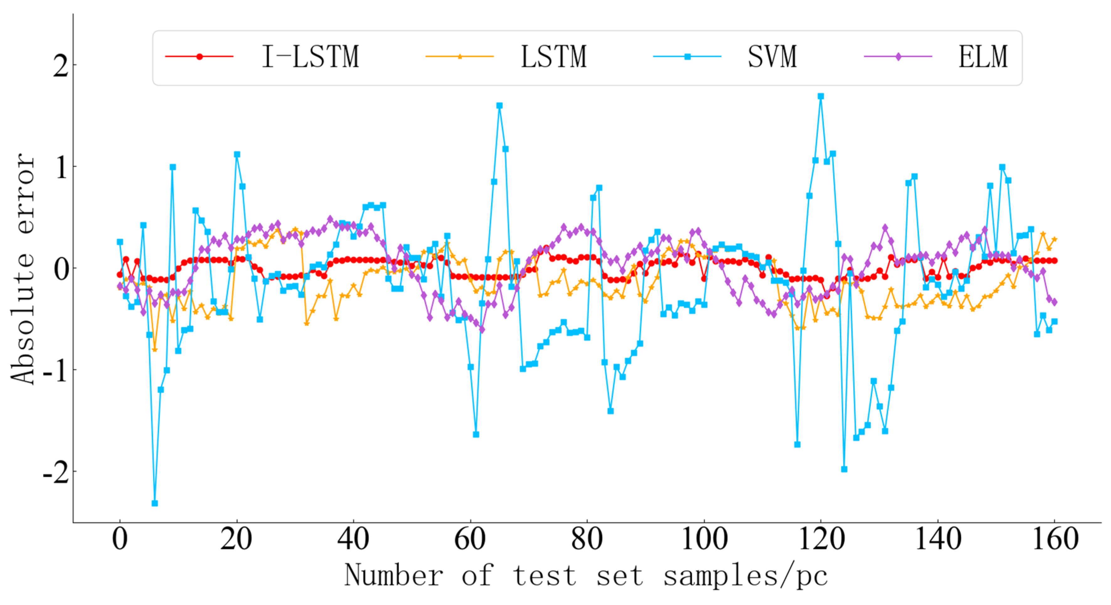
• Intelligent Flow Fitting Method: This method combined the hydraulic turbine model test data and actual operational data for flow characteristic curve fitting, using an I-LSTM. The I-LSTM method is compared with SVM, ELM and LSTM. The prediction results of SVM have a large error, but compared with ELM and LSTM, MSE is reduced by about 46% and 38%, respectively. MAE is reduced by about 25% and 21%, respectively. RMSE is reduced by about 27% and 24%, respectively. The fitting model covered the operational characteristics of the hydraulic turbines under various conditions and its actual operational characteristics
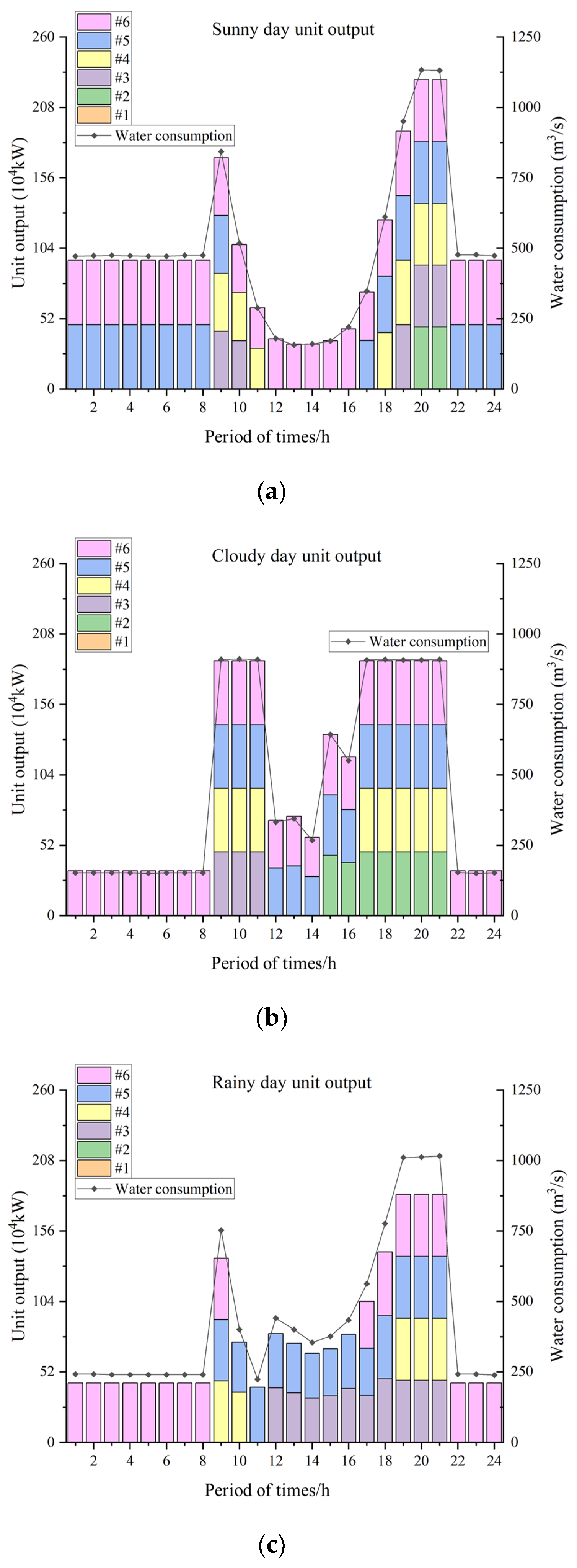
• Low-consumption Load-Distribution Strategy: The RF load-distribution model was compared with the traditional dynamic programming algorithm. The total water consumption of hydropower units in each scenario is reduced by 1.24%. Start and stop no more than twice. Maximum output fluctuation rate of no more than 3.3%. The maximum value of the non-economic operating zone is only 15.43%. It significantly improved the operational efficiency and resource-utilization rate of hydropower stations, and showcased the immense potential of intelligent and low-energy consumption strategies in the field of hydropower
• In the hydro-photovoltaic complementary system, the average efficiency of the hydropower station units using the RF algorithm for load allocation is more than 93% under the three scenarios of sunny, cloudy and rainy days. The total water consumption in the three scenarios is less than based on the dynamic programming algorithm for load allocation. In the hydro-photovoltaic complementary system with more constraints, the model is trained using the real operating data, and can effectively distribute the load under the existing conditions and make corresponding predictions for some additional conditions.

This study provided a new approach for the application of intelligent low-consumption optimization strategies in hydropower. However, to ensure the accuracy of the calculation results, the data requirement is quite large. In addition, the parameter settings of the algorithm will also have a significant impact on the results. Therefore, there are still some key technical details that need to be further processed and refined.

References

1. Shrestha, A.; Mustafa, A.A.; Htike, M.M.; You, V.; Kakinaka, M. Evolution of energy mix in emerging countries: Modern renewable energy, traditional renewable energy, and non-renewable energy. Renew. Energy 2022, 199, 419–432. [Google Scholar] [CrossRef]
2. Guidi, G.; Violante, A.C.; Iuliis, S.D. Environmental Impact of Electricity Generation Technologies: A Comparison between Conventional, Nuclear, and Renewable Technologies. Energies 2023, 16, 7847. [Google Scholar] [CrossRef]
3. Singh, V.K.; Signal, S.K. Operation of hydro power plants-a review. Renew. Sustain. Energy Rev. 2017, 69, 610–619. [Google Scholar] [CrossRef]
4. Kumar, K.; Saini, R.P. A review on operation and maintenance of hydropower plants. Sustain. Energy Technol. Assess. 2022, 49, 101704. [Google Scholar] [CrossRef]
5. Dauda, A.K.; Panda, A.; Mishra, U. Synergistic effect of complementary cleaner energy sources on controllable emission from hybrid power systems in optimal power flow framework. J. Clean. Prod. 2023, 419, 138290. [Google Scholar] [CrossRef]
6. Xia, L.; Zhu, Y.; Lai, C.; Huang, W.; Chen, S.; Wang, J. Research on the Hydropower Coupling-Based Hydropower Station Scheduling Optimization Model. J. Phys. Conf. Ser. 2021, 2005, 012140. [Google Scholar]
7. Gao, Y.; Xu, W.; Wang, Y.; Wen, X. Research on the Economic Operation of Large Hydropower Stations Based on Optimal Load Distribution Tables. Hydropower Energy Sci. 2023, 41, 197–201. [Google Scholar]
8. Yang, K.; Chen, L.; Li, H. Overall Spatio-Temporal Economic Operation Model and Its Algorithm for Large Hydropower Stations. J. Huazhong Univ. Sci. Technol. (Nat. Sci. Ed.) 2015, 43, 117–122. [Google Scholar]
9. Thaeer Hammid, A.; Awad, O.I.; Sulaiman, M.H.; Gunasekaran, S.S.; Mostafa, S.A.; Manoj Kumar, N.; Khalaf, B.A.; Al-Jawhar, Y.A.; Abdulhasan, R.A. A Review of Optimization Algorithms in Solving Hydro Generation Scheduling Problem. Energies 2020, 13, 2787. [Google Scholar] [CrossRef]
10. Xu, L.; Tian, J.; Qi, P.; Sun, S.; Li, X. Curve fitting and application of the operating characteristics of a hydraulic turbine based on MEA-BP. People’s Yangtze River 2019, 50, 141–145. [Google Scholar]
11. Guo, A.; Chang, J.; Yang, S.; Zhao, Y.; Wang, Y.; Fang, J. Time scale effect in dimension reduction optimal load distribution of hydropower generating units. Power Grid Technol. 2024, 1–10. [Google Scholar] [CrossRef]
12. Stefanizzi, M.; Capurso, T.; Balaccco, G.; Binetti, M.; Camporeale, S.M.; Torresi, M. Selection, control and techno-economic feasibility of Pumps as Turbines in Water Distribution Network. Renew. Energy 2020, 162, 1292–1306. [Google Scholar] [CrossRef]
13. Ma, W.; Yang, J.; Zhao, Z.; Yang, W.; Yang, J. Subdivision method of characteristic curve of Francis turbine under multiple boundary conditions. Trans. Chin. Soc. Agric. Eng. 2021, 37, 31–39. [Google Scholar]
14. Plua, F.A.; Sanchez-Romero, F.-J.; Hidalgo, V.; Lopez-Jimenez, P.A.; Perez-Sanchez, M. New Expressions to Apply the Variation Operation Strategy in Engineering Tools Using Pumps Working as Turbines. Mathematics 2021, 9, 860. [Google Scholar] [CrossRef]
15. Skjelbred, H.I.; Kong, J. A comparison of linear interpolation and spline interpolation for turbine efficiency curves in short-term hydropower scheduling problems. IOP Conf. Ser. Earth Environ. Sci. 2019, 240, 042011. [Google Scholar] [CrossRef]
16. Wu, Q.; Zhang, L.; Ma, Z. Extension and Reconstruction of Turbine Comprehensive Characteristic Curves Based on Engineering Experience and RBF Neural Network. J. Basic Sci. Eng. 2022, 27, 996–1007. [Google Scholar]
17. Liu, D.; Hu, X.; Zeng, Q.; Zhou, H.K.; Xiao, Z.H. Refined Model of Turbine Characteristic Curves Based on Input-Output Correction. J. Hydraul. Eng. 2019, 50, 555–564. [Google Scholar]
18. Li, J.; Chen, Q.; Chen, G. Research on BP Neural Network Fitting Method for Comprehensive Characteristic Curves of Hydraulic Turbines. J. Hydroelectr. Eng. 2015, 34, 182–188. [Google Scholar]
19. Li, J.; Han, C.; Yu, F. A New Processing Method Combined with BP Neural Network for Francis Turbine Synthetic Characteristic Curve Research. Int. J. Rotating Mach. 2017, 2017, 1870541. [Google Scholar] [CrossRef]
20. Li, M.; Wibowo, S.; Guo, W. Nonlinear Curve Fitting Using Extreme Learning Machines and Radial Basis Function Networks. Comput. Sci. Eng. 2019, 21, 6–15. [Google Scholar] [CrossRef]
21. Abritta, R.; Panoeiro, F.F.; De Aguiar, E.P.; Honorio, L.D.M.; Marcato, A.L.M.; da Silva Junior, I.C. Fuzzy system applied to a hydraulic turbine efficiency curve fitting. Electr. Eng. 2020, 102, 1361–1370. [Google Scholar] [CrossRef]
22. Schonlau, M.; Zou, R.Y. The random forest algorithm for statistical learning. Stata J. Promot. Commun. Stat. Stata 2020, 20, 3–29. [Google Scholar] [CrossRef]
23. Soydaner, D. A Comparison of Optimization Algorithms for Deep Learning. Int. J. Pattern Recognit. Artif. Intell. 2020, 34, 2052013. [Google Scholar] [CrossRef]
24. Bao, C.; Xie, J.; Zhang, Q.; Chen, F. Deep Learning-Based Encapsulation of Hydropower Unit Consumption Characteristics and Economic Operation within Hydropower Plants. Hydropower Energy Sci. 2022, 40, 173–177. [Google Scholar]
25. Alvarez, G.E. An Optimization Model for Operations of Large scale Hydro Power Plants. IEEE Lat. Am. Trans. 2020, 18, 1631–1638. [Google Scholar] [CrossRef]
26. Olofintoye, O.; Otieno, F.; Adeyemo, J. Real-time optimal water allocation for daily hydropower generation from the Vanderkloof dam, South Afric. Appl. Soft Comput. 2016, 47, 119–129. [Google Scholar] [CrossRef]
27. Amani, A.; Alizadeh, H. Solving Hydropower Unit Commitment Problem Using a Novel Sequential Mixed Integer Linear Programming Approach. Water Resour. Manag. 2021, 35, 1711–1729. [Google Scholar] [CrossRef]
28. Paredes, M.; Martins LS, A.; Soares, S. Using Semidefinite Relaxation to Solve the Day-Ahead Hydro Unit Commitment Problem. IEEE Trans. Power Syst. 2015, 30, 2695–2705. [Google Scholar] [CrossRef]
29. Finardi, E.C.; De Silva, E.L.; Sagastizábal, C. Solving the unit commitment problem of hydropower plants via Lagrangian Relaxation and Sequential Quadratic Programming. Comput. Appl. Math. 2005, 24, 317–342. [Google Scholar] [CrossRef]
30. Shang, Y.; Lu, S.; Gong, J.; Liu, R.; Li, X.; Fan, Q. Improved genetic algorithm for economic load dispatch in hydropower plants and comprehensive performance comparison with dynamic programming method. J. Hydrol. 2017, 554, 306–316. [Google Scholar] [CrossRef]
31. Yuan, Y.; Yuan, X. An improved PSO approach to short-term economic dispatch of cascaded hydropower plants. Kybernetes 2010, 39, 1359–1365. [Google Scholar] [CrossRef]
32. Zheng, J.; Yang, K.; Lu, X. Limited adaptive genetic algorithm for inner-plant economical operation of hydropower station. Hydrol. Res. 2013, 44, 583–599. [Google Scholar] [CrossRef]
33. Adarsh, B.R.; Raghunathan, T.; Jayabarathi, T.; Yang, X.-S. Economic dispatch using chaotic bat algorithm. Energy 2016, 96, 666–675. [Google Scholar] [CrossRef]
34. Villeneuve, Y.; Séguin, S.; Chehri, A. AI-Based Scheduling Models, Optimization, and Prediction for Hydropower Generation: Opportunities, Issues, and Future Direction. Energies 2023, 16, 3335. [Google Scholar] [CrossRef]
35. Li, P.; Liu, Y. Construction of Turbine Operating Characteristic Surface Based on Moving Least Squares Method. Hydropower Energy Sci. 2023, 41, 183–186+17. [Google Scholar]
36. Landi, F.; Baraldi, L.; Cornia, M.; Cucchiara, R. Working Memory Connections for LSTM. Neural Netw. 2021, 144, 334–341. [Google Scholar] [CrossRef] [PubMed]
37. Yao, L.; Pan, Z.; Ning, H. Unlabeled Short Text Similarity with LSTM Encoder. IEEE Access 2019, 7, 3430–3437. [Google Scholar] [CrossRef]
38. Wang, W.; Tong, M.; Yu, M. Blood Glucose Prediction with VMD and LSTM Optimized by Improved Particle Swarm Optimization. IEEE Access 2020, 8, 217908–217916. [Google Scholar] [CrossRef]
39. Biswas, T.K.; Giri, K.; Roy, S. ECKM: An improved K-means clustering based on computational geometry. Expert Syst. Appl. 2023, 212, 118862. [Google Scholar] [CrossRef]
40. Zhao, X. Realization of Intelligent Power Distribution Monitoring System Based on Data Mining Technology; Nanjing University of Posts and Telecommunications: Nanjing, China, 2021. [Google Scholar]
Figure 1. LSTM unit structure.
Mathematics 12 01292 g001
Figure 2. Test IPSO.
Mathematics 12 01292 g002
Figure 4. Unit load-distribution model based on Random Forest.
Mathematics 12 01292 g004
Figure 5. Changes in the fitness of the objective function.
Mathematics 12 01292 g005
Figure 6. Changes in the number of neurons.
Mathematics 12 01292 g006
Figure 7. Change in network learning rate.
Mathematics 12 01292 g007
Figure 8. Change in the number of network training iterations.
Mathematics 12 01292 g008
Figure 9. I-LSTM network prediction results.
Mathematics 12 01292 g009
Figure 10. Hydraulic turbine model experiments and real machine operating data.
Mathematics 12 01292 g010
Figure 11. The number of clustering centers determined.
Mathematics 12 01292 g011
Figure 12. Clustering results.
Mathematics 12 01292 g012
Figure 13. Random Forest Binary Tree Number Optimization.
Mathematics 12 01292 g013
Figure 14. Random Forest calculation results. (a) The output of each unit on sunny days; (b) The output of each unit on cloudy days; (c) The output of each unit on rainy days.
Mathematics 12 01292 g014
Figure 15. Operating Efficiency of Various Units in the Factory in June.
Mathematics 12 01292 g015