Comparisons of Numerical and Solitary Wave Solutions for the Stochastic Reaction–Diffusion Biofilm Model including Quorum Sensing

Abstract

This study deals with a stochastic reaction–diffusion biofilm model under quorum sensing. Quorum sensing is a process of communication between cells that permits bacterial communication about cell density and alterations in gene expression. This model produces two results: the bacterial concentration, which over time demonstrates the development and decomposition of the biofilm, and the biofilm bacteria collaboration, which demonstrates the potency of resistance and defense against environmental stimuli. In this study, we investigate numerical solutions and exact solitary wave solutions with the presence of randomness. The finite difference scheme is proposed for the sake of numerical solutions while the generalized Riccati equation mapping method is applied to construct exact solitary wave solutions. The numerical scheme is analyzed by checking consistency and stability. The consistency of the scheme is gained under the mean square sense while the stability condition is gained by the help of the Von Neumann criteria. Exact stochastic solitary wave solutions are constructed in the form of hyperbolic, trigonometric, and rational forms. Some solutions are plots in 3D and 2D form to show dark, bright and solitary wave solutions and the effects of noise as well. Mainly, the numerical results are compared with the exact solitary wave solutions with the help of unique physical problems. The comparison plots are dispatched in three dimensions and line representations as well as by selecting different values of parameters.

1. Introduction

Reaction–diffusion equations are models for the densities of substances or living things that disperse over space by Brownian motion, random walks, hydrodynamic turbulence, or other comparable mechanisms that react to one another and their environment in ways that affect their local densities. Even though they are essentially deterministic, reaction–diffusion models can be created as limits of stochastic processes with the right scaling [1]. Grzybowski in [1] proposed a modeling strategy that specifically enables us to convert presumptions about stochastic local movement into deterministic descriptions of global densities. Reaction–diffusion models approach time and space as continuous, describe population densities, and are spatially explicit. These characteristics set them apart from other categories of spatial models like metapopulation models, integrodifference models, and interacting particle systems [2]. The existence of a minimal patch size required to support a population, the presence of traveling wavefronts corresponding to biological invasions, and the emergence of spatial patterns are the three main ecological phenomena supported by reaction–diffusion equations [3]. Shi et al. worked on a multimodal hybrid parallel network intrusion detection model [4], and Zhang et al. worked on geometric landmarks and kinetic constraints [5,6]. Zou et al. were concerned with the Riemann–Hilbert approach for the higher-order Gerdjikov–Ivanov equation with nonzero boundary conditions [7]. Solhi et al. worked on stochastic fractional Volterra integro-differential equations by using the enhanced moving least squares method [8].

The two components of the mathematical model are an ordinary differential equation (ODE) that depicts quorum sensing among the bacteria and a reaction–diffusion equation, also referred to as a parabolic partial differential equation, that describes the formation of biofilms [9]. Bacteria communicate information about cell density and modify gene expression through the process of quorum sensing, which requires cell-to-cell communication. One well-known type of equation system that has been used to represent, for example, interactions between cellular processes like cell growth in mathematical biology is the reaction–diffusion–ODE model. This model produces two results: bacterial concentration, which over time demonstrates the development and decomposition of the biofilm, and biofilm bacteria collaboration, which demonstrates the potency of resistance and defense against environmental stimuli. [10]. Baber et al. investigated optimization and exact solutions for the for biofilm model [11]. But, in this study we will consider the biofilm model under the effects of noise and investigate the computational numerical results and solitary wave solutions. Mainly, we focused on comparing these results via simulations. So, this is described by the reaction–diffusion model and written as [12]

$$\begin{array}{ccc}\hfill X_t& =& \nabla ·(A\nabla X)+\alpha X(1-X/\beta )-\gamma (t,x)(1-Y)X\mathrm{in}D\times {\mathbb{R}}^{+},\hfill \end{array}$$

(1)

$$\begin{array}{ccc}\hfill Y_t& =& \xi max(0,arctan\left(X(q\left(X\right)-Y)\right))Y-k{Y}^2\mathrm{in}D\times {\mathbb{R}}^{+}.\hfill \end{array}$$

(2)

Here, $\nabla .(\nabla )=\frac{{\partial }^{2}X}{\partial x^2}$ and $max(0,arctan(X\left(q\right(X)-Y)\left)\right)=\sigma$ are the maximum function $(X,Y)$, where $Y(x,t)$ is the cooperation of the bacteria. $Y=0$ means no cooperation; $Y=1$ means maximal cooperation. The simplified form of the above system is taken as follows:

$$\begin{array}{ccc}\hfill X_t& =& A{X}_{xx}+\alpha X(1-\frac{1}{\beta }X)-\gamma (1-Y)X+{\nu }_{1}X{B}_t,\mathrm{in}D\times {\mathbb{R}}^{+},\hfill \end{array}$$

(3)

$$\begin{array}{ccc}\hfill Y_t& =& \xi \sigma Y-k{Y}^2+{\nu }_{2}Y{B}_t\mathrm{in}D\times {\mathbb{R}}^{+},\hfill \end{array}$$

(4)

where $X(x,t)$ is concentration of bacteria and the variable x denotes position. Since each bacteria has a fixed size, the values of $X(x,t)$ and $Y(x,t)$ represent cooperation and biofilm thickness, respectively. The population density in an x neighborhood at time t is measured by quorum functional k, and is employed in quorum sensing models; $q\left(X\right)$ is the quorum sense and $\gamma (x,t)$ is a function that is either spreading more quickly (bigger A) in a thinner biofilm that offers less protection due to less collaboration (smaller $\gamma$) or is spreading more slowly (smaller A) and constructing a more robust biofilm with greater cooperation (larger $\gamma$). Also, A is the relative size. Meanwhile, the positive constants that depend on the bacterial strain and the environment are $\alpha$, $\beta$, A, $\zeta$, and $\sigma$. It will be feasible to predict how a patient’s biofilm will evolve using these predictive parameters, allowing for the selection of the best course of action. Moreover, the noise control parameters are ${\nu }_1$ and ${\nu }_2$ along with $B_t$, which is the multiplicative time noise.

These days, stochastic modeling is a hot field of research. Many researchers are working on stochastic models, both numerically and analytically. There are various techniques for investigating the exact solitary wave and approximate solutions for nonlinear stochastic partial differential equations (SPDEs). The different numerical schemes include the forward Euler difference scheme [13], the non-standard finite difference scheme [14], the backward Euler difference scheme [15], the implicit finite difference scheme [16], the Crank–Nikolson finite difference scheme [17], etc. On the other hand, to find exact solutions many analytical techniques are used to explore exact solutions for nonlinear PDEs, such as the new modified extended direct algebraic method [18], the $G^{\prime }/G$-model expansion method [19], the Riccati equation mapping method [20], the Hirota bilinear method [21,22], the modified exponential rational function method [23], and the ${\varphi }^6$-model expansion method [24].

When we see most physical phenomena at the microscale and magnify them, these phenomena are stochastic or random phenomena. It is very natural to consider the differential equation, which has some kind of randomness involved. So, if this randomness is bounded in the solution of the differential equations, such problems are stochastic differential equations.

The numerical solution of the stochastic differential equation is not a simple job. It becomes more difficult when our governing equation is a nonlinear stochastic differential equation and we have tried to overcome such issues. We have used the numerical method. The proposed scheme is consistent with the given PDE, and it is conditionally stable and time efficient.

In this study, we mainly focus on numerical and exact solitary wave solutions under the noise effect. The reaction–diffusion biofilm model is analyzed under quorum sensing. Quorum sensing is the process of communication between cells that permits bacterial communication about cell density and alterations in gene expression. This model produces two results: bacterial concentration, which over time demonstrates the development and decomposition of the biofilm, and biofilm bacteria collaboration, which demonstrates the potency of resistance and defense against environmental stimuli. The numerical solutions are gained by a proposed finite difference scheme, more efficient than others. The advantages of the “Forward difference formula” are as follows: (i) it is easy to compute; (ii) it is time-efficient; (iii) high-efficiency computers are required for implicit methods, and for the forward method low-efficiency computers can be used. The analysis of the scheme, like consistency and stability, is checked to ensure how our scheme behaves. On the other hand, exact solitary wave solutions are gained by using the generalized Riccati equation mapping method. This method is easy to deal with and provides us trigonometric, hyperbolic, and rational solutions as well. In the present literature, researchers are dealing with the problems numerically and analytically separately. Therefore, there is a huge gap in the comparison of the results.

The novelty of this work is that we compare the numerical results with newly constructed soliton solutions. For the comparison of the results, the initial conditions (ICs) and boundary conditions (BCs) are required for the numerical purpose, so we construct the ICs and BCs by selecting the soliton solutions. The soliton solutions are compared with the numerical solution provided by the scheme, which gives us almost the same behaviors. These results are very helpful for the further study of the nonlinear reaction–diffusion models under the noise effect. Some main properties of the Brownian motion are presented in the next result.

Definition 1 

([25,26]). Wiener process and Itô integral: The Brownian motion ${\left\{B\left(t\right)\right\}}_{t\ge 0}$ is a stochastic process and fulfills the following properties:

1. 

$B\left(0\right)=0$ with probability 1;

2. 

$B\left(t\right)$ is the continuous function of $t\ge 0$;

3. 

$B\left(t_2\right)-B\left(t_1\right)$ and $B\left(t_4\right)-B\left(t_3\right)$ are independent increments for all $0\le t_1<t_2\le t_3<t_4$;

4. 

$B\left(t_2\right)-B\left(t_1\right)$, $B\left(t_4\right)-B\left(t_3\right)$ has normal distribution $N(0,(t_2-t_1),(t_4-t_3))$;

5. 

$\mathbf{E}\left|B_t\right|=0$ for each value $t\ge 0$, where $\mathbf{E}|·|$ represents the expected value of noise;

6. 

$\mathbf{E}\left|B_t^2\right|=t$ for each value $t\ge 0$;

7. 

$\mathbf{E}|B_t-B_s|=0$;

8. 

$\mathbf{E}\left|{(B_t-B_s)}^2\right|=t-s$.

2. Stochastic Finite Difference Scheme

This current sections deals with the proposed non-standard finite difference scheme (NSFDS). First, we divide the domain $x\in [0,L]$ and $t\in [0,T]$ into $M^2\times N$ with space and times stepsizes $\Delta x=\frac{L}{M}$ and $\Delta t=\frac{T}{N}$, respectively. Then, $x_{\varpi }=\frac{\varpi }{h}$, $\varpi =0,1,2,\dots ,M,$ and $t_{\kappa }=\frac{\kappa }{\Delta t}$, for $\kappa =0,1,2,\dots ,N.$

We approximate the continuous derivatives with a discrete approximation, such as

$$\begin{array}{c}\hfill X_t\approx \frac{X_{\varpi }^{\kappa +1}-X_{\varpi }^{\kappa }}{\Delta t},X_{xx}\approx \frac{X_{\varpi +1}^{\kappa }-2X_{\varpi }^{\kappa +1}+X_{\varpi -1}^{\kappa }}{\Delta x^2},\end{array}$$

(5)

Here, we suppose $\Delta t$ and $\Delta x$ are the time and space stepsizes, respectively. Putting the above approximations in (3)–(4), we obtain the NSFDS as follows:

$$\begin{array}{ccc}\hfill \left(1+2r_1+\frac{\alpha }{\beta }\Delta t{X}_{\varpi }^{\kappa }+\Delta t\gamma \right)X_{\varpi }^{\kappa +1}& =& r_1(X_{\varpi -1}^{\kappa }+X_{\varpi +1}^{\kappa })+(1+\alpha \Delta t+\Delta t\gamma Y_{\varpi }^{\kappa })X_{\varpi }^{\kappa }\hfill \\ & & +{\nu }_1{X}_{\varpi }^{\kappa }(B^{(\kappa +1)\Delta t}-B^{\kappa \Delta t})(1+\Delta tk{Y}_{\varpi }^{\kappa }),\hfill \end{array}$$

(6)

$$\begin{array}{ccc}\hfill Y_{\varpi }^{\kappa +1}& =& (1+\Delta t\zeta \sigma )Y_{\varpi }^{\kappa }+{\nu }_2{Y}_{\varpi }^{\kappa }(B^{(\kappa +1)\Delta t}-B^{\kappa \Delta t}).\hfill \end{array}$$

(7)

Here, $r_1=\frac{A\Delta t}{\Delta x^2}$, $X_{\varpi }^{\kappa }$ and $Y_{\varpi }^{\kappa }$ are the approximations of the state variables $X(x,t)$ and $Y(x,t)$ at the point $(\varpi \Delta x,\kappa t)$, respectively. So, this is the required NSFD scheme of the system (3)–(4).

Consistency of Schemes

In this section, we discuss the consistence of the proposed NSFD schemes (6)–(7).

Theorem 1. 

The proposed NSFD schemes (6)–(7) are consistent in the mean square sense for X and Y.

Proof. 

For scheme (6), $X(x,t)$ is the smooth function, so we suppose an operator $\Theta \left(X\right)={\int }_{\kappa \Delta t}^{(\kappa +1)\Delta t}$. Applying this operator on (3), we obtain (see [27])

$$\begin{array}{ccc}\hfill \Theta {\left(X\right)}_{\varpi }^{\kappa }& =& X(\varpi \Delta x,(\kappa +1)\Delta t)-X(\varpi \Delta x,\kappa \Delta t)+A{\int }_{\kappa \Delta t}^{(\kappa +1)\Delta t}{X}_{xx}(\kappa \Delta x,\rho )d\rho \hfill \\ & & +\alpha {\int }_{\kappa \Delta t}^{(\kappa +1)\Delta t}X(\kappa \Delta x,\rho )d\rho -\frac{\alpha }{\beta }{\int }_{\kappa \Delta t}^{(\kappa +1)\Delta t}X{(\kappa \Delta x,\rho )}^{2}d\rho -\gamma {\int }_{\kappa \Delta t}^{(\kappa +1)\Delta t}X(\kappa \Delta x,\rho )d\rho \hfill \\ & & +\gamma {\int }_{\kappa \Delta t}^{(\kappa +1)\Delta t}Y(\kappa \Delta x,\rho )d\rho X(\kappa \Delta x,\rho )d\rho +{\nu }_1{\int }_{\kappa \Delta t}^{(\kappa +1)\Delta t}{X(\kappa \Delta x,\rho )dB|}_{\rho },\hfill \end{array}$$

(8)

and, therefore,

$$\begin{array}{ccc}\hfill {\Theta |}_{\varpi }^{\kappa }\left(X\right)& =& X(\varpi \Delta x,(\kappa +1)\Delta t)-X(\varpi \Delta x,\kappa \Delta t)+A\frac{X_{\varpi +1}^{\kappa }-2X_{\varpi }^{\kappa +1}+X_{\varpi -1}^{\kappa }}{\Delta x^2}\hfill \\ & & +\alpha X(\varpi \Delta x,\kappa \Delta t)-\frac{\alpha }{\beta }{\left(X(\varpi \Delta x,\kappa \Delta t)\right)}^2-\gamma X(\varpi \Delta x,\kappa \Delta t)\hfill \\ & & +\gamma X(\varpi \Delta x,\kappa \Delta t)Y(\varpi \Delta x,\kappa \Delta t)+{\nu }_{1}X(\varpi \Delta x,\kappa \Delta t)(B^{(\kappa +1)\Delta t}-B^{\kappa \Delta }).\hfill \end{array}$$

(9)

Then,

$$\begin{array}{ccc}\hfill \mathbf{E}|\Theta {\left(X\right)}_{\varpi }^{\kappa }{-\Theta |}_{\varpi }^{\kappa }\left(X\right){|}^2& \le & \mathbf{E}|{\int }_{\kappa \Delta t}^{(\kappa +1)\Delta t}A\left(X_{xx}(\kappa \Delta x,\rho )-\frac{X_{\varpi +1}^{\kappa }-2X_{\varpi }^{\kappa +1}+X_{\varpi -1}^{\kappa }}{\Delta x^2}\right)d\rho {|}^2\hfill \\ & & +\alpha \mathbf{E}|{\int }_{\kappa \Delta t}^{(\kappa +1)\Delta t}\left(X(\kappa \Delta x,\rho )-X(\varpi \Delta x,\kappa \Delta t)\right)d\rho {|}^2\hfill \\ & & -\frac{\alpha }{\beta }\mathbf{E}|{\int }_{\kappa \Delta t}^{(\kappa +1)\Delta t}\left(X{(\kappa \Delta x,\rho )}^2-X{(\varpi \Delta x,\kappa \Delta t)}^2\right)d\rho {|}^2\hfill \\ & & -\gamma \mathbf{E}|{\int }_{\kappa \Delta t}^{(\kappa +1)\Delta t}\left(X(\kappa \Delta x,\rho )-X(\kappa \Delta x,\rho )\right)d\rho {|}^2\hfill \\ & & +\gamma \mathbf{E}|{\int }_{\kappa \Delta t}^{(\kappa +1)\Delta t}\left(Y(\kappa \Delta x,\rho )d\rho X(\kappa \Delta x,\rho )-Y(\kappa \Delta x,\rho )d\rho X(\kappa \Delta x,\rho )\right)d\rho {|}^2\hfill \\ & & +{\nu }_1\mathbf{E}|{\int }_{\kappa \Delta t}^{(\kappa +1)\Delta t}\left(X(\kappa \Delta x,\rho )-X(\kappa \Delta x,\rho )\right){dB|}_{\rho }{|}^2,\hfill \end{array}$$

(10)

using the property of the Itô integral we obtain

$$\begin{array}{ccc}\hfill \mathbf{E}|\Theta {\left(X\right)}_{\varpi }^{\kappa }{-\Theta |}_{\varpi }^{\kappa }\left(X\right){|}^2& \le & \mathbf{E}|{\int }_{\kappa \Delta t}^{(\kappa +1)\Delta t}A\left(X_{xx}(\kappa \Delta x,\rho )-\frac{X_{\varpi +1}^{\kappa }-2X_{\varpi }^{\kappa +1}+X_{\varpi -1}^{\kappa }}{\Delta x^2}\right)d\rho {|}^2\hfill \\ & & +\alpha \mathbf{E}|{\int }_{\kappa \Delta t}^{(\kappa +1)\Delta t}\left(X(\kappa \Delta x,\rho )-X(\varpi \Delta x,\kappa \Delta t)\right)d\rho {|}^2\hfill \\ & & -\frac{\alpha }{\beta }\mathbf{E}|{\int }_{\kappa \Delta t}^{(\kappa +1)\Delta t}\left(X{(\kappa \Delta x,\rho )}^2-X{(\varpi \Delta x,\kappa \Delta t)}^2\right)d\rho {|}^2\hfill \\ & & -\gamma \mathbf{E}|{\int }_{\kappa \Delta t}^{(\kappa +1)\Delta t}\left(X(\kappa \Delta x,\rho )-X(\kappa \Delta x,\rho )\right)d\rho {|}^2\hfill \\ & & +\gamma \mathbf{E}|{\int }_{\kappa \Delta t}^{(\kappa +1)\Delta t}\left(Y(\kappa \Delta x,\rho )d\rho X(\kappa \Delta x,\rho )-Y(\kappa \Delta x,\rho )d\rho X(\kappa \Delta x,\rho )\right)d\rho {|}^2\hfill \\ & & +{\nu }_1{\int }_{\kappa \Delta t}^{(\kappa +1)\Delta t}\mathbf{E}|\left(X(\kappa \Delta x,\rho )-X(\kappa \Delta x,\rho )\right){|}^{2}d\rho .\hfill \end{array}$$

(11)

So, $\mathbf{E}|\Theta {\left(Y\right)}_{\varpi }^{\kappa }{-\Theta |}_{\varpi }^{\kappa }\left(Y\right)|\to 0$ as $\Delta x\to \infty$, $\Delta t\to \infty$. Hence, the proposed scheme is consistent with (3).

For scheme (6), $Y(x,t)$ is the smooth function, so we suppose the same operator $\Theta \left(Y\right)={\int }_{\kappa \Delta t}^{(\kappa +1)\Delta t}$. Applying this operator on (4), we obtain the following form:

$$\begin{array}{ccc}\hfill \Theta {\left(Y\right)}_{\varpi }^{\kappa }& =& Y(\varpi \Delta x,(\kappa +1)\Delta t)-Y(\varpi \Delta x,\kappa \Delta t)+\sigma \zeta {\int }_{\kappa \Delta t}^{(\kappa +1)\Delta t}Y(\kappa \Delta x,\rho )d\rho \hfill \\ & & -k{\int }_{\kappa \Delta t}^{(\kappa +1)\Delta t}Y{(\kappa \Delta x,\rho )}^{2}d\rho +{\nu }_2{\int }_{\kappa \Delta t}^{(\kappa +1)\Delta t}{Y(\kappa \Delta x,\rho )dB|}_{\rho },\hfill \end{array}$$

(12)

and

$$\begin{array}{ccc}\hfill {\Theta |}_{\varpi }^{\kappa }\left(Y\right)& =& Y(\varpi \Delta x,(\kappa +1)\Delta t)-Y(\varpi \Delta x,\kappa \Delta t)+\sigma \zeta {\int }_{\kappa \Delta t}^{(\kappa +1)\Delta t}Y(\kappa \Delta x,\rho )d\rho \hfill \\ & & -k{\int }_{\kappa \Delta t}^{(\kappa +1)\Delta t}Y{(\kappa \Delta x,\rho )}^{2}d\rho +{\nu }_2{\int }_{\kappa \Delta t}^{(\kappa +1)\Delta t}{Y(\kappa \Delta x,\rho )dB|}_{\rho }.\hfill \end{array}$$

(13)

Then,

$$\begin{array}{ccc}\hfill \mathbf{E}|\Theta {\left(Y\right)}_{\varpi }^{\kappa }{-\Theta |}_{\varpi }^{\kappa }\left(Y\right){|}^2& \le & \sigma \zeta \mathbf{E}|{\int }_{\kappa \Delta t}^{(\kappa +1)\Delta t}\left(Y(\kappa \Delta x,\rho )-Y(\kappa \Delta x,\rho )\right)d\rho {|}^2\hfill \\ & & -k\mathbf{E}|{\int }_{\kappa \Delta t}^{(\kappa +1)\Delta t}\left(Y{(\kappa \Delta x,\rho )}^2-Y{(\kappa \Delta x,\rho )}^2\right)d\rho {|}^2\hfill \\ & & +{\nu }_2\mathbf{E}|{\int }_{\kappa \Delta t}^{(\kappa +1)\Delta t}\left(Y(\kappa \Delta x,\rho )-Y(\kappa \Delta x,\rho )\right){dB|}_{\rho }{|}^2,\hfill \end{array}$$

(14)

and using the property of the Itô integral we obtain

$$\begin{array}{ccc}\hfill \mathbf{E}|\Theta {\left(Y\right)}_{\varpi }^{\kappa }{-\Theta |}_{\varpi }^{\kappa }\left(Y\right){|}^2& \le & \sigma \zeta \mathbf{E}|{\int }_{\kappa \Delta t}^{(\kappa +1)\Delta t}\left(Y(\kappa \Delta x,\rho )-Y(\kappa \Delta x,\rho )\right)d\rho {|}^2\hfill \\ & & -k\mathbf{E}|{\int }_{\kappa \Delta t}^{(\kappa +1)\Delta t}\left(Y{(\kappa \Delta x,\rho )}^2-Y{(\kappa \Delta x,\rho )}^2\right)d\rho {|}^2\hfill \\ & & +{\nu }_2{\int }_{\kappa \Delta t}^{(\kappa +1)\Delta t}\mathbf{E}|\left(Y(\kappa \Delta x,\rho )-Y(\kappa \Delta x,\rho )\right){|}^{2}d\rho .\hfill \end{array}$$

(15)

Again, $\mathbf{E}|\Theta {\left(Y\right)}_{\varpi }^{\kappa }{-\Theta |}_{\varpi }^{\kappa }\left(Y\right)|\to 0$ as $\Delta x\to \infty$, $\Delta t\to \infty$. Hence, the proposed scheme is consistent with (4). □

3. Stability of Schemes

In this section, our purpose is to find the stability condition for the proposed NSFD schemes (6)–(7). The Von Neumann criteria were used to prove their stability. Suppose the general approximation of a differential equation such as

$$\begin{array}{c}\hfill X_{\varpi ,\kappa }={\varphi }_1\left(t\right)e^{i\left(\rho x\right)}.\end{array}$$

(16)

Replacing this expression into the schemes, and after simplification, we obtain the amplification factor (the expected value in a mean square sense) as follows:

$$\begin{array}{c}\hfill \mathbf{E}|\frac{{\varphi }_1(t+\Delta t)}{{\varphi }_1\left(t\right)}{|}^2\le 1+\chi \Delta t,\end{array}$$

(17)

where $\chi$ is a constant. So, this is the required stability condition for the proposed schemes.

Theorem 2. 

Proposed scheme (6)–(7) is stable.

Proof. 

To find the stability conditions for schemes (6)–(7), we linearize (6) by using the Von Neumann criteria,

$$\begin{array}{c}\hfill \left(1+2r_1+\Delta t\gamma \right)X_{\varpi }^{\kappa +1}=r_1(X_{\varpi -1}^{\kappa }+X_{\varpi +1}^{\kappa })+(1+\alpha \Delta t)X_{\varpi }^{\kappa }+{\nu }_1{X}_{\varpi }^{\kappa }(B^{(\kappa +1)\Delta t}-B^{\kappa \Delta t}).\end{array}$$

(18)

By replacing supposition (16) in (18), we obtain

$$\begin{array}{c}\hfill \left(1+2r_1+\Delta t\gamma \right){\varphi }_1(t+\Delta t)e^{i\left(\rho x\right)}=\left(r_1(e^{i\rho \Delta x}+e^{-i\rho \Delta x})+(1+\alpha \Delta t)+{\nu }_1(B^{(\kappa +1)\Delta t}-B^{\kappa \Delta t})\right){\varphi }_1\left(t\right)e^{i\left(\rho x\right)}.\end{array}$$

Now, we take the expectations $\mathbf{E}$ on both sides,

$$\begin{array}{c}\hfill \mathbf{E}|\frac{{\varphi }_1(t+\Delta t)}{{\varphi }_1\left(t\right)}{|}^2=|\frac{1+\alpha \Delta t+2r_1(1-2{sin}^2\left(\frac{\rho x}{2}\right))}{1+2r_1+\gamma \Delta t}{|}^2+|\frac{{\nu }_1}{1+2r_1+\gamma \Delta t}{|}^2(B^{(\kappa +1)\Delta t}-B^{\kappa \Delta t}),\end{array}$$

(19)

where X is independent from the state of the Wiener process. Thus, we obtain

$$\begin{array}{c}\hfill \mathbf{E}|\frac{{\varphi }_1(t+\Delta t)}{{\varphi }_1\left(t\right)}{|}^2=|\frac{1+\alpha \Delta t+2r_1(1-2{sin}^2\left(\frac{\rho x}{2}\right))}{1+2r_1+\gamma \Delta t}{|}^2+|\frac{{\nu }_1}{1+2r_1+\gamma \Delta t}{|}^2\Delta t,\end{array}$$

(20)

also

$$|\frac{1+\alpha \Delta t+2r_1(1-2{sin}^2\left(\frac{\rho x}{2}\right))}{1+2r_1+\gamma \Delta t}{|}^2\le 1,$$

and

$$|\frac{{\nu }_1}{1+2r_1+\gamma \Delta t}{|}^2=\delta .$$

Then, we obtain

$$\begin{array}{c}\hfill \mathbf{E}|\frac{{\varphi }_1(t+\Delta t)}{{\varphi }_1\left(t\right)}{|}^2\le 1+\delta \Delta t.\end{array}$$

(21)

Further, we linearize (7), with the help of the Von Neumann criteria, as

$$\begin{array}{c}\hfill Y_{\varpi }^{\kappa +1}=(1+\Delta t\zeta \sigma )Y_{\varpi }^{\kappa }+{\nu }_2{Y}_{\varpi }^{\kappa }(B^{(\kappa +1)\Delta t}-B^{\kappa \Delta t}).\end{array}$$

(22)

Let us replace again (16) and obtain

$$\begin{array}{c}\hfill {\varphi }_2(t+\Delta t)e^{i\left(\rho x\right)}=\left(1+\Delta t\zeta \sigma +{\nu }_2(B^{(\kappa +1)\Delta t}-B^{\kappa \Delta t})\right){\varphi }_2\left(t\right)e^{i\left(\rho x\right)}.\end{array}$$

Then,

$$\begin{array}{c}\hfill \mathbf{E}|\frac{{\varphi }_2(t+\Delta t)}{{\varphi }_2\left(t\right)}{|}^2=|1+\Delta t\zeta \sigma {|}^2+|{\nu }_2{|}^2(B^{(\kappa +1)\Delta t}-B^{\kappa \Delta t}),\end{array}$$

(23)

where Y is independent from the state of the Wiener process. Thus, we obtain

$$\begin{array}{c}\hfill \mathbf{E}|\frac{{\varphi }_2(t+\Delta t)}{{\varphi }_2\left(t\right)}{|}^2=|1+\Delta t\zeta \sigma {|}^2+|{\nu }_2{|}^2\Delta t,\end{array}$$

(24)

also, $|1+\Delta t\zeta \sigma {|}^2\le 1$ and $|{\nu }_2{|}^2=\delta$. Then, we obtain

$$\begin{array}{c}\hfill \mathbf{E}|\frac{{\varphi }_2(t+\Delta t)}{{\varphi }_2\left(t\right)}{|}^2\le 1+\delta \Delta t.\end{array}$$

(25)

So, the proposed schemes are stable. □

4. General Procedure of Generalized Riccati Equation Mapping Method

The generalized Riccati equation mapping method is defined in the following steps [20,28,29].

4.1. Step I

Given a nonlinear partial differential equation (NPDE) with the independent variables $t,x$ and dependence variable u, such as

$$\begin{array}{c}\hfill \Omega (u,u_t,u_x,u_{xx},u_{xt},u_{tt}\dots )=0,\end{array}$$

(26)

where the dependent variable’s subscripts stand for the partial derivatives and $\Omega$ is typically a polynomial function of its argument.

4.2. Step II

By using the wave transformation, Equation (26) has the following ansatz:

$$\begin{array}{c}\hfill u=\varphi \left(\rho \right),\mathrm{where}\rho =\alpha x+\beta t,\end{array}$$

(27)

where $\rho$ is a real function to be determined. Substituting Equation (27) into Equation (26) then we obtain an ordinary differential equation (ODE) as

$$\begin{array}{c}\hfill Q(\varphi ,{\varphi }_{\rho },{\varphi }_{\rho \rho },\dots )=0.\end{array}$$

(28)

4.3. Step III

Suppose that the solution of Equation (28) is in the polynomial form

$$\begin{array}{c}\hfill \varphi \left(\rho \right)=\sum _{j=0}^M{\nu }_{j}J{\left(\rho \right)}^j,\end{array}$$

(29)

where ${\nu }_j$ are constants that are determined later and M is a positive integer that is obtained by the help of the balancing principle. $J\left(\rho \right)$ represents the solution of the given generalized Riccati equation:

$$\begin{array}{c}\hfill J^{\prime }\left(\rho \right)=\zeta +\theta J\left(\rho \right)+\kappa J^2\left(\rho \right),\end{array}$$

(30)

where $\zeta$, $\theta$ and $\kappa$ are all real constants. Substituting Equation (29) with Equation (30) into the relevant ODE and vanishing all the coefficients of $J^j\left(\rho \right)$ will yield a system of algebraic equations, from which we can obtain the parameters ${\nu }_j,=(j=1,\dots ,n)$ and $\rho$. Solving the algebraic equations, with the known solutions of Equation (30), one can easily obtain the non-travelling wave solutions to the NPDE (26). We can obtain the 27 solutions to Equation (28) that are in Appendix A.

5. Stochastic Exact Solutions

The stochastic wave transform is now used to obtain the exact solitary wave solutions for the stochastic biofilm system (3)–(4), such as [25,30,31]:

$$\begin{array}{c}\hfill X(x,t)=\varphi \left(\rho \right)e^{{\nu }_{1}B\left(t\right)-\frac{{\nu }_1^2}{2}t},Y(x,t)=\psi \left(\rho \right)e^{{\nu }_{2}B\left(t\right)-\frac{{\nu }_2^2}{2}t},\mathrm{where}\rho =x-ct,\end{array}$$

(31)

being $\varphi$ and $\psi$ the deterministic functions, while c is the speed of light and ${\nu }_1$, ${\nu }_2$ are the noise strength for the Brownian motion. Their derivatives are defined, such as

$$\begin{array}{ccc}\hfill X_t& =& \left(-c{\varphi }^{\prime }+{\nu }_1\varphi B_t-\frac{{\nu }_1^2}{2}\varphi +\frac{{\nu }_1^2}{2}\varphi \right)e^{{\nu }_{1}B\left(t\right)-\frac{{\nu }_1^2}{2}t},\hfill \\ \hfill Y_t& =& \left(-c{\psi }^{\prime }+{\nu }_2\psi B_t-\frac{{\nu }_2^2}{2}\psi +\frac{{\nu }_2^2}{2}\psi \right)e^{{\nu }_{2}B\left(t\right)-\frac{{\nu }_2^2}{2}t},\hfill \\ \hfill X_{xx}& =& {\varphi }^{″}{e}^{{\nu }_{1}B\left(t\right)-\frac{{\nu }_1^2}{2}t},\hfill \end{array}$$

where $\frac{{\nu }_1^2}{2}\varphi \left(\rho \right)$ and $\frac{{\nu }_2^2}{2}\psi \left(\rho \right)$ are referred to the Itô term. Putting these derivatives into system (3)–(4), we obtain an ODE form, such as

$$\begin{array}{ccc}& & c{\varphi }^{\prime }-{\nu }_1\varphi B_t+\frac{{\nu }_1^2}{2}\varphi -\frac{{\nu }_1^2}{2}\varphi +{\varphi }^{″}+\alpha \varphi -\frac{\alpha }{\beta }{\varphi }^2{e}^{{\nu }_{1}B\left(t\right)-\frac{{\nu }_1^2}{2}t}-\gamma \varphi +\gamma \varphi \psi e^{{\nu }_{2}B\left(t\right)-\frac{{\nu }_2^2}{2}t}+{\nu }_1\varphi B_t=0,\hfill \end{array}$$

(32)

$$\begin{array}{ccc}& & c{\psi }^{\prime }-{\nu }_2\psi B_t+\frac{{\nu }_2^2}{2}\psi -\frac{{\nu }_2^2}{2}\psi +\zeta \sigma \psi +k{\psi }^2{e}^{{\nu }_{2}B\left(t\right)-\frac{{\nu }_2^2}{2}t}+{\nu }_2\psi B_t=0.\hfill \end{array}$$

(33)

By taking the expectation on both expressions,

$$\begin{array}{ccc}& & c{\varphi }^{\prime }+{\varphi }^{″}+\alpha \varphi -\frac{\alpha }{\beta }{\varphi }^2{e}^{{\nu }_{1}B\left(t\right)}{e}^{-\frac{{\nu }_1^2}{2}t}-\gamma \varphi +\gamma \varphi \psi e^{{\nu }_{2}B\left(t\right)}{e}^{-\frac{{\nu }_2^2}{2}t}=0,\hfill \end{array}$$

(34)

$$\begin{array}{ccc}& & c{\psi }^{\prime }+\zeta \sigma \psi +k{\psi }^2{e}^{{\nu }_{2}B\left(t\right)}{e}^{-\frac{{\nu }_2^2}{2}t}=0.\hfill \end{array}$$

(35)

Since $\mathbf{E}\left(e^{\delta Z}\right)$ (for every real number $\delta$ and Z) is the standard normal random variable, then identities are $\mathbf{E}\left(e^{{\nu }_{1}B\left(t\right)}\right)=e^{\frac{{\nu }_1^2}{2}t}$ and $\mathbf{E}\left(e^{{\nu }_{2}B\left(t\right)}\right)=e^{\frac{{\nu }_2^2}{2}t}$. So, (34)–(35) are expressed as

$$\begin{array}{ccc}& & c{\varphi }^{\prime }+{\varphi }^{″}+\alpha \varphi -\frac{\alpha }{\beta }{\varphi }^2-\gamma \varphi +\gamma \varphi \psi =0,\hfill \end{array}$$

(36)

$$\begin{array}{ccc}& & c{\psi }^{\prime }+\zeta \sigma \psi +k{\psi }^2=0,\hfill \end{array}$$

(37)

where $\varphi$ and $\psi$ are the polynomials and their derivatives are in respect to $\rho$. In the next section, we apply the generalized Riccati equation mapping (GREM) method to obtain the stochastic exact solitary wave solutions for the stochastic biofilm system (3)–(4).

Generalized Riccati Equation Mapping (GREM) Method

In this subsection, we use the generalized Riccati equation mapping (GREM) method to gain the exact stochastic wave solutions. This method provides us with the dark-, bright-, exponential- and periodic-form solutions. Let us define the general solution in the polynomial form of (36)–(37). For further details, see [20,28,29]:

$$\begin{array}{ccc}\hfill \varphi \left(\rho \right)& =& \sum _{j=0}^{M_1}{\nu }_j{J}^j\left(\rho \right),{\nu }_j\ne 0,\hfill \end{array}$$

(38)

$$\begin{array}{ccc}\hfill \psi \left(\rho \right)& =& \sum _{j=0}^{M_2}{\tau }_j{J}^j\left(\rho \right),{\tau }_j\ne 0,\hfill \end{array}$$

(39)

Here, ${\nu }_j,{\tau }_j(0\le j\le M_i)$, $i=1,2$ are constants (to be determined later) and $J^i\left(\rho \right)$$i=1,2,\dots ,M_i$, $i=1,2$ satisfy the Equations (36) and (37) that we take as follows:

$$\begin{array}{c}\hfill J^{\prime }\left(\rho \right)=\zeta +\theta J\left(\rho \right)+\kappa J^2\left(\rho \right).\end{array}$$

(40)

By using the homogeneous balancing principle, the number of summands in (36) is $M_1=2$ while from (37) it is $M_2=1$. We replace these values in (38)–(39) and obtain

$$\begin{array}{ccc}\hfill \varphi \left(\rho \right)& =& {\nu }_0+{\nu }_{1}J\left(\rho \right)+{\nu }_2{J}^2\left(\rho \right),\hfill \end{array}$$

(41)

$$\begin{array}{ccc}\hfill \psi \left(\rho \right)& =& {\tau }_0+{\tau }_{1}J\left(\rho \right).\hfill \end{array}$$

(42)

By calculating the derivatives of (41)–(42) and replacing (40) into (38)–(39), we obtain a system of algebraic equations. This system is solved by means of Mathematica 11.1 and we obtain the unknown constants,

$$\begin{array}{ccc}\hfill {\nu }_0& =& \frac{{\alpha }^2\beta +\alpha \beta \gamma {\tau }_0-\alpha \beta \gamma +A_1}{2{\alpha }^2},\hfill \\ \hfill {\nu }_1& =& 0,\hfill \\ \hfill {\nu }_2& =& \frac{6A\beta {\kappa }^2}{\alpha },\hfill \\ \hfill c& =& \frac{10A\theta \kappa +\gamma {\tau }_1}{2\kappa },\hfill \end{array}$$

where $A_1=\sqrt{{\left({\alpha }^2\beta +\alpha \beta \gamma {\tau }_0-\alpha \beta \gamma \right)}^2+48{\alpha }^2{A}^2{\beta }^2{\zeta }^2{\kappa }^2}.$ Meanwhile, the constant values for (37) are

$$\begin{array}{ccc}\hfill {\tau }_0& =& \frac{-A_2+4\zeta \kappa k\xi \sigma +{\theta }^2(-k)\xi \sigma }{2\left(4\zeta \kappa k^2-{\theta }^2{k}^2\right)},\hfill \\ \hfill {\tau }_1& =& \frac{\kappa A_2}{k^2\left({\theta }^3-4\zeta \theta \kappa \right)},\hfill \\ \hfill c& =& \frac{\theta k{\xi }^2{\sigma }^2}{A_2},\hfill \end{array}$$

where $A_2=\sqrt{{\theta }^2{k}^2{\xi }^2{\sigma }^2\left({\theta }^2-4\zeta \kappa \right)}.$

Substituting these constants in (38)–(39), we obtain the solutions of Equations (36) and (37). Then, by replacing the transformation in these solutions, we obtain different hyperbolic, trigonometric, and rational solutions of (3)–(4).

Family-I: When the condition ${\theta }^2-4\zeta \kappa >0$ is satisfied and $\zeta \kappa \ne 0$, then different hyperbolic solutions are extracted:

$$\begin{array}{ccc}\hfill X_1(x,t)& =& \left(\frac{{\alpha }^2\beta +\alpha \beta \gamma {\tau }_0-\alpha \beta \gamma +A_1}{2{\alpha }^2}+\frac{3A\beta }{2\alpha }\right.\hfill \\ & & \left.{\left(\sqrt{{\theta }^2-4\zeta \kappa }tanh\left(\frac{1}{2}\sqrt{{\theta }^2-4\zeta \kappa }\left(x-\frac{t\left(10A\theta \kappa +\gamma {\tau }_1\right)}{2\kappa }\right)\right)+\theta \right)}^2\right)e^{{\nu }_{1}B\left(t\right)-\frac{{\nu }_1^2}{2}t},\hfill \end{array}$$

(43)

$$\begin{array}{ccc}\hfill Y_1(x,t)& =& \left(\frac{-A_2+4\zeta \kappa k\xi \sigma +{\theta }^2(-k)\xi \sigma }{2\left(4\zeta \kappa k^2-{\theta }^2{k}^2\right)}-\frac{A_2}{2k^2\left({\theta }^3-4\zeta \theta \kappa \right)}\right.\hfill \\ & & \left.\left(\theta +\sqrt{{\theta }^2-4\zeta \kappa }tanh\left(\frac{1}{2}\sqrt{{\theta }^2-4\zeta \kappa }\left(x-\frac{\theta k{\xi }^2{\sigma }^{2}t}{A_2}\right)\right)\right)\right)e^{{\nu }_{2}B\left(t\right)-\frac{{\nu }_2^2}{2}t},\hfill \end{array}$$

(44)

$$\begin{array}{ccc}\hfill X_2(x,t)& =& \left(\frac{{\alpha }^2\beta +\alpha \beta \gamma {\tau }_0-\alpha \beta \gamma +A_1}{2{\alpha }^2}+\frac{3A\beta }{2\alpha }\right.\hfill \\ & & \left.{\left(\sqrt{{\theta }^2-4\zeta \kappa }coth\left(\frac{1}{2}\sqrt{{\theta }^2-4\zeta \kappa }\left(x-\frac{t\left(10A\theta \kappa +\gamma {\tau }_1\right)}{2\kappa }\right)\right)+\theta \right)}^2\right)e^{{\nu }_{1}B\left(t\right)-\frac{{\nu }_1^2}{2}t},\hfill \end{array}$$

(45)

$$\begin{array}{ccc}\hfill Y_2(x,t)& =& \left(\frac{-A_2+4\zeta \kappa k\xi \sigma +{\theta }^2(-k)\xi \sigma }{2\left(4\zeta \kappa k^2-{\theta }^2{k}^2\right)}-\frac{A_2}{2k^2\left({\theta }^3-4\zeta \theta \kappa \right)}\right.\hfill \\ & & \left.\left(\theta +\sqrt{{\theta }^2-4\zeta \kappa }coth\left(\frac{1}{2}\sqrt{{\theta }^2-4\zeta \kappa }\left(x-\frac{\theta k{\xi }^2{\sigma }^{2}t}{A_2}\right)\right)\right)\right)e^{{\nu }_{2}B\left(t\right)-\frac{{\nu }_2^2}{2}t},\hfill \end{array}$$

(46)

$$\begin{array}{ccc}\hfill X_3(x,t)& =& \left(\frac{{\alpha }^2\beta +\alpha \beta \gamma {\tau }_0-\alpha \beta \gamma +A_1}{2{\alpha }^2}+\frac{3A\beta }{2\alpha }\right.\hfill \\ & & \left(\theta +\sqrt{{\theta }^2-4\zeta \kappa }\left(tanh\left(\sqrt{{\theta }^2-4\zeta \kappa }\left(x-\frac{t\left(10A\theta \kappa +\gamma {\tau }_1\right)}{2\kappa }\right)\right)\right.\right.\hfill \\ & & \left.{\left.\left.+i\mathrm{sech}\left(\sqrt{{\theta }^2-4\zeta \kappa }\left(x-\frac{t\left(10A\theta \kappa +\gamma {\tau }_1\right)}{2\kappa }\right)\right)\right)\right)}^2\right)e^{{\nu }_{1}B\left(t\right)-\frac{{\nu }_1^2}{2}t},\hfill \end{array}$$

(47)

$$\begin{array}{ccc}\hfill Y_3(x,t)& =& \left(\frac{-A_2+4\zeta \kappa k\xi \sigma +{\theta }^2(-k)\xi \sigma }{2\left(4\zeta \kappa k^2-{\theta }^2{k}^2\right)}-\frac{A_2}{2k^2\left({\theta }^3-4\zeta \theta \kappa \right)}\right.\hfill \\ & & \left(\theta +\sqrt{{\theta }^2-4\zeta \kappa }\left(tanh\left(\sqrt{{\theta }^2-4\zeta \kappa }\left(x-\frac{\theta k{\xi }^2{\sigma }^{2}t}{A_2}\right)\right)\right.\right.\hfill \\ & & \left.\left.\left.+i\mathrm{sech}\left(\sqrt{{\theta }^2-4\zeta \kappa }\left(x-\frac{\theta k{\xi }^2{\sigma }^{2}t}{A_2}\right)\right)\right)\right)\right)e^{{\nu }_{2}B\left(t\right)-\frac{{\nu }_2^2}{2}t},\hfill \end{array}$$

(48)

$$\begin{array}{ccc}\hfill X_4(x,t)& =& \left(\frac{{\alpha }^2\beta +\alpha \beta \gamma {\tau }_0-\alpha \beta \gamma +A_1}{2{\alpha }^2}+\frac{3A\beta }{2\alpha }\right.\hfill \\ & & \left(\sqrt{{\theta }^2-4\zeta \kappa }\left(coth\left(\sqrt{{\theta }^2-4\zeta \kappa }\left(x-\frac{t\left(10A\theta \kappa +\gamma {\tau }_1\right)}{2\kappa }\right)\right)\right.\right.\hfill \\ & & \left.{\left.\left.+\mathrm{csch}\left(\sqrt{{\theta }^2-4\zeta \kappa }\left(x-\frac{t\left(10A\theta \kappa +\gamma {\tau }_1\right)}{2\kappa }\right)\right)\right)+\theta \right)}^2\right)e^{{\nu }_{1}B\left(t\right)-\frac{{\nu }_1^2}{2}t},\hfill \end{array}$$

(49)

$$\begin{array}{ccc}\hfill Y_4(x,t)& =& \left(\frac{-A_2+4\zeta \kappa k\xi \sigma +{\theta }^2(-k)\xi \sigma }{2\left(4\zeta \kappa k^2-{\theta }^2{k}^2\right)}-\frac{A_2}{2k^2\left({\theta }^3-4\zeta \theta \kappa \right)}\right.\hfill \\ & & \left(\theta +\sqrt{{\theta }^2-4\zeta \kappa }\left(coth\left(\sqrt{{\theta }^2-4\zeta \kappa }\left(x-\frac{\theta k{\xi }^2{\sigma }^{2}t}{A_2}\right)\right)\right.\right.\hfill \\ & & \left.\left.\left.+\mathrm{csch}\left(\sqrt{{\theta }^2-4\zeta \kappa }\left(x-\frac{\theta k{\xi }^2{\sigma }^{2}t}{A_2}\right)\right)\right)\right)\right)e^{{\nu }_{2}B\left(t\right)-\frac{{\nu }_2^2}{2}t},\hfill \end{array}$$

(50)

$$\begin{array}{ccc}\hfill X_5(x,t)& =& \left(\frac{{\alpha }^2\beta +\alpha \beta \gamma {\tau }_0-\alpha \beta \gamma +A_1}{2{\alpha }^2}+\frac{3A\beta }{8\alpha }\right.\hfill \\ & & \left(\sqrt{{\theta }^2-4\zeta \kappa }\left(tanh\left(\frac{1}{4}\sqrt{{\theta }^2-4\zeta \kappa }\left(x-\frac{t\left(10A\theta \kappa +\gamma {\tau }_1\right)}{2\kappa }\right)\right)\right.\right.\hfill \\ & & \left.{\left.\left.+coth\left(\frac{1}{4}\sqrt{{\theta }^2-4\zeta \kappa }\left(x-\frac{t\left(10A\theta \kappa +\gamma {\tau }_1\right)}{2\kappa }\right)\right)\right)+2\theta \right)}^2\right)e^{{\nu }_{1}B\left(t\right)-\frac{{\nu }_1^2}{2}t},\hfill \end{array}$$

(51)

$$\begin{array}{ccc}\hfill Y_5(x,t)& =& \left(\frac{-A_2+4\zeta \kappa k\xi \sigma +{\theta }^2(-k)\xi \sigma }{2\left(4\zeta \kappa k^2-{\theta }^2{k}^2\right)}-\frac{A_2}{4k^2\left({\theta }^3-4\zeta \theta \kappa \right)}\right.\hfill \\ & & \left(2\theta +\sqrt{{\theta }^2-4\zeta \kappa }\left(tanh\left(\frac{1}{4}\sqrt{{\theta }^2-4\zeta \kappa }\left(x-\frac{\theta k{\xi }^2{\sigma }^{2}t}{A_2}\right)\right)\right.\right.\hfill \\ & & \left.\left.\left.+coth\left(\frac{1}{4}\sqrt{{\theta }^2-4\zeta \kappa }\left(x-\frac{\theta k{\xi }^2{\sigma }^{2}t}{A_2}\right)\right)\right)\right)\right)e^{{\nu }_{2}B\left(t\right)-\frac{{\nu }_2^2}{2}t},\hfill \end{array}$$

(52)

$$\begin{array}{ccc}\hfill X_6(x,t)& =& \left(\frac{{\alpha }^2\beta +\alpha \beta \gamma {\tau }_0-\alpha \beta \gamma +A_1}{2{\alpha }^2}+\frac{3A\beta }{2\alpha }\right.\hfill \\ & & \left.{\left(\frac{\sqrt{\left(G^2+H^2\right)\left({\theta }^2-4\zeta \kappa \right)}-G\sqrt{{\theta }^2-4\zeta \kappa }cosh\left(\sqrt{{\theta }^2-4\zeta \kappa }\left(x-\frac{t\left(10A\theta \kappa +\gamma {\tau }_1\right)}{2\kappa }\right)\right)}{Gsinh\left(\sqrt{{\theta }^2-4\zeta \kappa }\left(x-\frac{t\left(10A\theta \kappa +\gamma {\tau }_1\right)}{2\kappa }\right)\right)+H}-\theta \right)}^2\right)e^{{\nu }_{1}B\left(t\right)-\frac{{\nu }_1^2}{2}t},\hfill \end{array}$$

(53)

$$\begin{array}{ccc}\hfill Y_6(x,t)& =& \left(\frac{-A_2+4\zeta \kappa k\xi \sigma +{\theta }^2(-k)\xi \sigma }{2\left(4\zeta \kappa k^2-{\theta }^2{k}^2\right)}+\frac{A_2}{2k^2\left({\theta }^3-4\zeta \theta \kappa \right)}\right.\hfill \\ & & \left.\left(\frac{\sqrt{\left(G^2+H^2\right)\left({\theta }^2-4\zeta \kappa \right)}-G\sqrt{{\theta }^2-4\zeta \kappa }cosh\left(B\right)}{Gsinh\left(\sqrt{{\theta }^2-4\zeta \kappa }\left(x-\frac{\theta k{\xi }^2{\sigma }^{2}t}{A_2}\right)\right)+H}-\theta \right)\right)e^{{\nu }_{2}B\left(t\right)-\frac{{\nu }_2^2}{2}t},\hfill \end{array}$$

(54)

where $B=\sqrt{{\theta }^2-4\zeta \kappa }\left(x-\frac{\theta k{\xi }^2{\sigma }^{2}t}{A_2}\right).$

$$\begin{array}{ccc}\hfill X_7(x,t)& =& \left(\frac{{\alpha }^2\beta +\alpha \beta \gamma {\tau }_0-\alpha \beta \gamma +A_1}{2{\alpha }^2}+\frac{3A\beta }{2\alpha }\right.\hfill \\ & & \left.{\left(-\frac{G\sqrt{{\theta }^2-4\zeta \kappa }cosh\left(\sqrt{{\theta }^2-4\zeta \kappa }\left(x-\frac{t\left(10A\theta \kappa +\gamma {\tau }_1\right)}{2\kappa }\right)\right)+\sqrt{\left(H^2-G^2\right)\left({\theta }^2-4\zeta \kappa \right)}}{Gsinh\left(\sqrt{{\theta }^2-4\zeta \kappa }\left(x-\frac{t\left(10A\theta \kappa +\gamma {\tau }_1\right)}{2\kappa }\right)\right)+H}-\theta \right)}^2\right)e^{{\nu }_{1}B\left(t\right)-\frac{{\nu }_1^2}{2}t},\hfill \end{array}$$

(55)

$$\begin{array}{ccc}\hfill Y_7(x,t)& =& \left(\frac{-A_2+4\zeta \kappa k\xi \sigma +{\theta }^2(-k)\xi \sigma }{2\left(4\zeta \kappa k^2-{\theta }^2{k}^2\right)}+\frac{A_2}{2k^2\left({\theta }^3-4\zeta \theta \kappa \right)}\right.\hfill \\ & & \left.\left(-\frac{\sqrt{\left(H^2-G^2\right)\left({\theta }^2-4\zeta \kappa \right)}+G\sqrt{{\theta }^2-4\zeta \kappa }cosh\left(B\right)}{Gsinh\left(\sqrt{{\theta }^2-4\zeta \kappa }\left(x-\frac{\theta k{\xi }^2{\sigma }^{2}t}{A_2}\right)\right)+H}-\theta \right)\right)e^{{\nu }_{2}B\left(t\right)-\frac{{\nu }_2^2}{2}t},\hfill \end{array}$$

(56)

where $G^2+H^2>0$ and $B=\sqrt{{\theta }^2-4\zeta \kappa }\left(x-\frac{\theta k{\xi }^2{\sigma }^{2}t}{A_2}\right)$ are the constants.

$$\begin{array}{ccc}\hfill X_8(x,t)& =& \left(\frac{{\alpha }^2\beta +\alpha \beta \gamma {\tau }_0-\alpha \beta \gamma +A_1}{2{\alpha }^2}\right.\hfill \\ & & \left.+\frac{24A\beta {\zeta }^2{\kappa }^2{cosh}^2\left(\frac{1}{2}\sqrt{{\theta }^2-4\zeta \kappa }\left(x-\frac{t\left(10A\theta \kappa +\gamma {\tau }_1\right)}{2\kappa }\right)\right)}{\alpha {\left(\sqrt{{\theta }^2-4\zeta \kappa }sinh\left(\frac{1}{2}\sqrt{{\theta }^2-4\zeta \kappa }\left(x-\frac{t\left(10A\theta \kappa +\gamma {\tau }_1\right)}{2\kappa }\right)\right)-\theta cosh\left(Z\right)\right)}^2}\right)e^{{\nu }_{1}B\left(t\right)-\frac{{\nu }_1^2}{2}t},\hfill \end{array}$$

(57)

where $Z=\frac{1}{2}\sqrt{{\theta }^2-4\zeta \kappa }\left(x-\frac{t\left(10A\theta \kappa +\gamma {\tau }_1\right)}{2\kappa }\right)$ and

$$\begin{array}{ccc}\hfill Y_8(x,t)& =& \left(\frac{-A_2+4\zeta \kappa k\xi \sigma +{\theta }^2(-k)\xi \sigma }{2\left(4\zeta \kappa k^2-{\theta }^2{k}^2\right)}\right.\hfill \\ & & \left.+\frac{2\zeta \kappa A_{2}cosh\left(\frac{1}{2}\sqrt{{\theta }^2-4\zeta \kappa }\left(x-\frac{\theta k{\xi }^2{\sigma }^{2}t}{A_2}\right)\right)}{k^2\left({\theta }^3-4\zeta \theta \kappa \right)\left(\sqrt{{\theta }^2-4\zeta \kappa }sinh\left(B\right)-\theta cosh\left(B\right)\right)}\right)e^{{\nu }_{2}B\left(t\right)-\frac{{\nu }_2^2}{2}t},\hfill \end{array}$$

(58)

where $B=\frac{1}{2}\sqrt{{\theta }^2-4\zeta \kappa }\left(x-\frac{\theta k{\xi }^2{\sigma }^{2}t}{A_2}\right).$

$$\begin{array}{ccc}\hfill X_9(x,t)& =& \left(\frac{{\alpha }^2\beta +\alpha \beta \gamma {\tau }_0-\alpha \beta \gamma +A_1}{2{\alpha }^2}\right.\hfill \\ & & \left.+\frac{24A\beta {\zeta }^2{\kappa }^2{sinh}^2\left(\frac{1}{2}\sqrt{{\theta }^2-4\zeta \kappa }\left(x-\frac{t\left(10A\theta \kappa +\gamma {\tau }_1\right)}{2\kappa }\right)\right)}{\alpha {\left(\theta sinh\left(\frac{1}{2}\sqrt{{\theta }^2-4\zeta \kappa }\left(x-\frac{t\left(10A\theta \kappa +\gamma {\tau }_1\right)}{2\kappa }\right)\right)-\sqrt{{\theta }^2-4\zeta \kappa }cosh\left(Z\right)\right)}^2}\right)e^{{\nu }_{1}B\left(t\right)-\frac{{\nu }_1^2}{2}t},\hfill \end{array}$$

(59)

where $Z=\frac{1}{2}\sqrt{{\theta }^2-4\zeta \kappa }\left(x-\frac{t\left(10A\theta \kappa +\gamma {\tau }_1\right)}{2\kappa }\right)$, and

$$\begin{array}{ccc}\hfill Y_9(x,t)& =& \left(\frac{-A_2+4\zeta \kappa k\xi \sigma +{\theta }^2(-k)\xi \sigma }{2\left(4\zeta \kappa k^2-{\theta }^2{k}^2\right)}\right.\hfill \\ & & \left.-\frac{2\zeta \kappa A_{2}sinh\left(\frac{1}{2}\sqrt{{\theta }^2-4\zeta \kappa }\left(x-\frac{\theta k{\xi }^2{\sigma }^{2}t}{A_2}\right)\right)}{k^2\left({\theta }^3-4\zeta \theta \kappa \right)\left(\theta sinh\left(B\right)-\sqrt{{\theta }^2-4\zeta \kappa }cosh\left(B\right)\right)}\right)e^{{\nu }_{2}B\left(t\right)-\frac{{\nu }_2^2}{2}t},\hfill \end{array}$$

(60)

where $B=\frac{1}{2}\sqrt{{\theta }^2-4\zeta \kappa }\left(x-\frac{\theta k{\xi }^2{\sigma }^{2}t}{A_2}\right).$

$$\begin{array}{ccc}\hfill X_{10}(x,t)& =& \left(\frac{{\alpha }^2\beta +\alpha \beta \gamma {\tau }_0-\alpha \beta \gamma +A_1}{2{\alpha }^2}\right.\hfill \\ & & \left.+\frac{24A\beta {\zeta }^2{\kappa }^2{cosh}^2\left(\sqrt{{\theta }^2-4\zeta \kappa }\left(x-\frac{t\left(10A\theta \kappa +\gamma {\tau }_1\right)}{2\kappa }\right)\right)}{\alpha {\left(\sqrt{{\theta }^2-4\zeta \kappa }sinh\left(\sqrt{{\theta }^2-4\zeta \kappa }\left(x-\frac{t\left(10A\theta \kappa +\gamma {\tau }_1\right)}{2\kappa }\right)\right)-\theta cosh\left(Z\right)-i\sqrt{{\theta }^2-4\zeta \kappa }\right)}^2}\right)e^{{\nu }_{1}B\left(t\right)-\frac{{\nu }_1^2}{2}t},\hfill \end{array}$$

(61)

being $Z=\sqrt{{\theta }^2-4\zeta \kappa }\left(x-\frac{t\left(10A\theta \kappa +\gamma {\tau }_1\right)}{2\kappa }\right)$, and

$$\begin{array}{ccc}\hfill Y_{10}(x,t)& =& \left(\frac{-A_2+4\zeta \kappa k\xi \sigma +{\theta }^2(-k)\xi \sigma }{2\left(4\zeta \kappa k^2-{\theta }^2{k}^2\right)}\right.\hfill \\ & & \left.+\frac{2\zeta \kappa A_{2}cosh\left(B\right)}{k^2\left({\theta }^3-4\zeta \theta \kappa \right)\left(-i\sqrt{{\theta }^2-4\zeta \kappa }+\sqrt{{\theta }^2-4\zeta \kappa }sinh\left(B\right)-\theta cosh\left(B\right)\right)}\right)e^{{\nu }_{2}B\left(t\right)-\frac{{\nu }_2^2}{2}t},\hfill \end{array}$$

(62)

where $B=\sqrt{{\theta }^2-4\zeta \kappa }\left(x-\frac{\theta k{\xi }^2{\sigma }^{2}t}{A_2}\right).$

$$\begin{array}{ccc}\hfill X_{11}(x,t)& =& \left(\frac{{\alpha }^2\beta +\alpha \beta \gamma {\tau }_0-\alpha \beta \gamma +A_1}{2{\alpha }^2}\right.\hfill \\ & & \left.+\frac{24A\beta {\zeta }^2{\kappa }^2{sinh}^2\left(\sqrt{{\theta }^2-4\zeta \kappa }\left(x-\frac{t\left(10A\theta \kappa +\gamma {\tau }_1\right)}{2\kappa }\right)\right)}{\alpha {\left(-\theta sinh\left(Z\right)+\sqrt{{\theta }^2-4\zeta \kappa }cosh\left(Z\right)+\sqrt{{\theta }^2-4\zeta \kappa }\right)}^2}\right)e^{{\nu }_{1}B\left(t\right)-\frac{{\nu }_1^2}{2}t},\hfill \end{array}$$

(63)

where $Z=\sqrt{{\theta }^2-4\zeta \kappa }\left(x-\frac{t\left(10A\theta \kappa +\gamma {\tau }_1\right)}{2\kappa }\right)$, and

$$\begin{array}{ccc}\hfill Y_{11}(x,t)& =& \left(\frac{-A_2+4\zeta \kappa k\xi \sigma +{\theta }^2(-k)\xi \sigma }{2\left(4\zeta \kappa k^2-{\theta }^2{k}^2\right)}\right.\hfill \\ & & \left.+\frac{2\zeta \kappa A_{2}sinh\left(B\right)}{k^2\left({\theta }^3-4\zeta \theta \kappa \right)\left(\sqrt{{\theta }^2-4\zeta \kappa }-\theta sinh\left(B\right)+\sqrt{{\theta }^2-4\zeta \kappa }cosh\left(B\right)\right)}\right)e^{{\nu }_{2}B\left(t\right)-\frac{{\nu }_2^2}{2}t},\hfill \end{array}$$

(64)

where $B=\sqrt{{\theta }^2-4\zeta \kappa }\left(x-\frac{\theta k{\xi }^2{\sigma }^{2}t}{A_2}\right).$

$$\begin{array}{ccc}\hfill X_{12}(x,t)& =& \left(\frac{{\alpha }^2\beta +\alpha \beta \gamma {\tau }_0-\alpha \beta \gamma +A_1}{2{\alpha }^2}\right.\hfill \\ & & \left.+\frac{96A\beta {\zeta }^2{\kappa }^2{sinh}^2\left(Z\right){cosh}^2\left(\frac{1}{4}\sqrt{{\theta }^2-4\zeta \kappa }\left(x-\frac{t\left(10A\theta \kappa +\gamma {\tau }_1\right)}{2\kappa }\right)\right)}{\alpha {\left(2\sqrt{{\theta }^2-4\zeta \kappa }{cosh}^2\left(Z\right)-2\theta sinh\left(Z\right)cosh\left(Z\right)-\sqrt{{\theta }^2-4\zeta \kappa }\right)}^2}\right)e^{{\nu }_{1}B\left(t\right)-\frac{{\nu }_1^2}{2}t},\hfill \end{array}$$

(65)

where $Z=\frac{1}{4}\sqrt{{\theta }^2-4\zeta \kappa }\left(x-\frac{t\left(10A\theta \kappa +\gamma {\tau }_1\right)}{2\kappa }\right)$, and

$$\begin{array}{ccc}\hfill Y_{12}(x,t)& =& \left(\frac{-A_2+4\zeta \kappa k\xi \sigma +{\theta }^2(-k)\xi \sigma }{2\left(4\zeta \kappa k^2-{\theta }^2{k}^2\right)}\right.\hfill \\ & & \left.+\frac{4\zeta \kappa A_{2}sinh\left(B\right)cosh\left(B\right)}{k^2\left({\theta }^3-4\zeta \theta \kappa \right)\left(-\sqrt{{\theta }^2-4\zeta \kappa }+2\sqrt{{\theta }^2-4\zeta \kappa }{cosh}^2\left(B\right)-2\theta sinh\left(B\right)cosh\left(B\right)\right)}\right)e^{{\nu }_{2}B\left(t\right)-\frac{{\nu }_2^2}{2}t},\hfill \end{array}$$

(66)

being $B=\frac{1}{4}\sqrt{{\theta }^2-4\zeta \kappa }\left(x-\frac{\theta k{\xi }^2{\sigma }^{2}t}{A_2}\right).$

Family-II: When ${\theta }^2-4\zeta \kappa <0$ and $\zeta \kappa \ne 0$, the trigonometric solutions of PDE (3)–(4) are as follows:

$$\begin{array}{ccc}\hfill X_{13}(x,t)& =& \left(\frac{{\alpha }^2\beta +\alpha \beta \gamma {\tau }_0-\alpha \beta \gamma +A_1}{2{\alpha }^2}+\frac{3A\beta }{2\alpha }\right.\hfill \\ & & \left.{\left(\sqrt{4\zeta \kappa -{\theta }^2}tan\left(\frac{1}{2}\sqrt{4\zeta \kappa -{\theta }^2}\left(x-\frac{t\left(10A\theta \kappa +\gamma {\tau }_1\right)}{2\kappa }\right)\right)-\theta \right)}^2\right)e^{{\nu }_{1}B\left(t\right)-\frac{{\nu }_1^2}{2}t},\hfill \end{array}$$

(67)

$$\begin{array}{ccc}\hfill Y_{13}(x,t)& =& \left(\frac{-A_2+4\zeta \kappa k\xi \sigma +{\theta }^2(-k)\xi \sigma }{2\left(4\zeta \kappa k^2-{\theta }^2{k}^2\right)}+\frac{A_2}{2k^2\left({\theta }^3-4\zeta \theta \kappa \right)}\right.\hfill \\ & & \left.\left(\sqrt{4\zeta \kappa -{\theta }^2}tan\left(\frac{1}{2}\sqrt{4\zeta \kappa -{\theta }^2}\left(x-\frac{\theta k{\xi }^2{\sigma }^{2}t}{A_2}\right)\right)-\theta \right)\right)e^{{\nu }_{2}B\left(t\right)-\frac{{\nu }_2^2}{2}t},\hfill \end{array}$$

(68)

$$\begin{array}{ccc}\hfill X_{14}(x,t)& =& \left(\frac{{\alpha }^2\beta +\alpha \beta \gamma {\tau }_0-\alpha \beta \gamma +A_1}{2{\alpha }^2}+\frac{3A\beta }{2\alpha }\right.\hfill \\ & & \left.{\left(\sqrt{4\zeta \kappa -{\theta }^2}cot\left(\frac{1}{2}\sqrt{4\zeta \kappa -{\theta }^2}\left(x-\frac{t\left(10A\theta \kappa +\gamma {\tau }_1\right)}{2\kappa }\right)\right)+\theta \right)}^2\right)e^{{\nu }_{1}B\left(t\right)-\frac{{\nu }_1^2}{2}t},\hfill \end{array}$$

(69)

$$\begin{array}{ccc}\hfill Y_{14}(x,t)& =& \left(\frac{-A_2+4\zeta \kappa k\xi \sigma +{\theta }^2(-k)\xi \sigma }{2\left(4\zeta \kappa k^2-{\theta }^2{k}^2\right)}-\frac{A_2}{2k^2\left({\theta }^3-4\zeta \theta \kappa \right)}\right.\hfill \\ & & \left.\left(\theta +\sqrt{4\zeta \kappa -{\theta }^2}cot\left(\frac{1}{2}\sqrt{4\zeta \kappa -{\theta }^2}\left(x-\frac{\theta k{\xi }^2{\sigma }^{2}t}{A_2}\right)\right)\right)\right)e^{{\nu }_{2}B\left(t\right)-\frac{{\nu }_2^2}{2}t},\hfill \end{array}$$

(70)

$$\begin{array}{ccc}\hfill X_{15}(x,t)& =& \left(\frac{{\alpha }^2\beta +\alpha \beta \gamma {\tau }_0-\alpha \beta \gamma +A_1}{2{\alpha }^2}+\frac{3A\beta }{2\alpha }\right.\hfill \\ & & \left(\sqrt{4\zeta \kappa -{\theta }^2}\left(tan\left(\sqrt{4\zeta \kappa -{\theta }^2}\left(x-\frac{t\left(10A\theta \kappa +\gamma {\tau }_1\right)}{2\kappa }\right)\right)\right.\right.\hfill \\ & & \left.{\left.\left.-sec\left(\sqrt{4\zeta \kappa -{\theta }^2}\left(x-\frac{t\left(10A\theta \kappa +\gamma {\tau }_1\right)}{2\kappa }\right)\right)\right)-\theta \right)}^2\right)e^{{\nu }_{1}B\left(t\right)-\frac{{\nu }_1^2}{2}t},\hfill \end{array}$$

(71)

$$\begin{array}{ccc}\hfill Y_{15}(x,t)& =& \left(\frac{-A_2+4\zeta \kappa k\xi \sigma +{\theta }^2(-k)\xi \sigma }{2\left(4\zeta \kappa k^2-{\theta }^2{k}^2\right)}+\frac{A_2}{2k^2\left({\theta }^3-4\zeta \theta \kappa \right)}\right.\hfill \\ & & \left(\sqrt{4\zeta \kappa -{\theta }^2}\left(tan\left(\sqrt{4\zeta \kappa -{\theta }^2}\left(x-\frac{\theta k{\xi }^2{\sigma }^{2}t}{A_2}\right)\right)\right.\right.\hfill \\ & & \left.\left.\left.-sec\left(\sqrt{4\zeta \kappa -{\theta }^2}\left(x-\frac{\theta k{\xi }^2{\sigma }^{2}t}{A_2}\right)\right)\right)-\theta \right)\right)e^{{\nu }_{2}B\left(t\right)-\frac{{\nu }_2^2}{2}t},\hfill \end{array}$$

(72)

$$\begin{array}{ccc}\hfill X_{16}(x,t)& =& \left(\frac{{\alpha }^2\beta +\alpha \beta \gamma {\tau }_0-\alpha \beta \gamma +A_1}{2{\alpha }^2}+\frac{3A\beta }{2\alpha }\right.\hfill \\ & & \left(\sqrt{4\zeta \kappa -{\theta }^2}\left(cot\left(\sqrt{4\zeta \kappa -{\theta }^2}\left(x-\frac{t\left(10A\theta \kappa +\gamma {\tau }_1\right)}{2\kappa }\right)\right)\right.\right.\hfill \\ & & \left.{\left.\left.-csc\left(\sqrt{4\zeta \kappa -{\theta }^2}\left(x-\frac{t\left(10A\theta \kappa +\gamma {\tau }_1\right)}{2\kappa }\right)\right)\right)+\theta \right)}^2\right)e^{{\nu }_{1}B\left(t\right)-\frac{{\nu }_1^2}{2}t},\hfill \end{array}$$

(73)

$$\begin{array}{ccc}\hfill Y_{16}(x,t)& =& \left(\frac{-A_2+4\zeta \kappa k\xi \sigma +{\theta }^2(-k)\xi \sigma }{2\left(4\zeta \kappa k^2-{\theta }^2{k}^2\right)}-\frac{A_2}{2k^2\left({\theta }^3-4\zeta \theta \kappa \right)}\right.\hfill \\ & & \left(\theta +\sqrt{4\zeta \kappa -{\theta }^2}\left(cot\left(\sqrt{4\zeta \kappa -{\theta }^2}\left(x-\frac{\theta k{\xi }^2{\sigma }^{2}t}{A_2}\right)\right)\right.\right.\hfill \\ & & \left.\left.\left.-csc\left(\sqrt{4\zeta \kappa -{\theta }^2}\left(x-\frac{\theta k{\xi }^2{\sigma }^{2}t}{A_2}\right)\right)\right)\right)\right)e^{{\nu }_{2}B\left(t\right)-\frac{{\nu }_2^2}{2}t},\hfill \end{array}$$

(74)

$$\begin{array}{ccc}\hfill X_{17}(x,t)& =& \left(\frac{{\alpha }^2\beta +\alpha \beta \gamma {\tau }_0-\alpha \beta \gamma +A_1}{2{\alpha }^2}+\frac{3A\beta }{8\alpha }\right.\hfill \\ & & \left(\sqrt{4\zeta \kappa -{\theta }^2}\left(tan\left(\frac{1}{4}\sqrt{4\zeta \kappa -{\theta }^2}\left(-\frac{t\left(10A\theta \kappa +\gamma {\tau }_1\right)}{2\kappa }+x\right)\right)\right.\right.\hfill \\ & & \left.{\left.\left.-cot\left(\frac{1}{4}\sqrt{4\zeta \kappa -{\theta }^2}\left(-\frac{t\left(10A\theta \kappa +\gamma {\tau }_1\right)}{2\kappa }+x+\right)\right)\right)-2\theta \right)}^2\right)e^{{\nu }_{1}B\left(t\right)-\frac{{\nu }_1^2}{2}t},\hfill \end{array}$$

(75)

$$\begin{array}{ccc}\hfill Y_{17}(x,t)& =& \left(\frac{-A_2+4\zeta \kappa k\xi \sigma +{\theta }^2(-k)\xi \sigma }{2\left(4\zeta \kappa k^2-{\theta }^2{k}^2\right)}+\frac{A_2}{4k^2\left({\theta }^3-4\zeta \theta \kappa \right)}\right.\hfill \\ & & \left(\sqrt{4\zeta \kappa -{\theta }^2}\left(tan\left(\frac{1}{4}\sqrt{4\zeta \kappa -{\theta }^2}\left(x-\frac{\theta k{\xi }^2{\sigma }^{2}t}{A_2}\right)\right)\right.\right.\hfill \\ & & \left.\left.\left.-cot\left(\frac{1}{4}\sqrt{4\zeta \kappa -{\theta }^2}\left(x-\frac{\theta k{\xi }^2{\sigma }^{2}t}{A_2}\right)\right)\right)-2\theta \right)\right)e^{{\nu }_{2}B\left(t\right)-\frac{{\nu }_2^2}{2}t},\hfill \end{array}$$

(76)

$$\begin{array}{ccc}\hfill X_{18}(x,t)& =& \left(\frac{{\alpha }^2\beta +\alpha \beta \gamma {\tau }_0-\alpha \beta \gamma +A_1}{2{\alpha }^2}+\frac{3A\beta }{2\alpha }\right.\hfill \\ & & \left.{\left(\frac{\sqrt{\left(G^2-H^2\right)\left(4\zeta \kappa -{\theta }^2\right)}-G\sqrt{4\zeta \kappa -{\theta }^2}cos\left(\sqrt{4\zeta \kappa -{\theta }^2}\left(x-\frac{t\left(10A\theta \kappa +\gamma {\tau }_1\right)}{2\kappa }\right)\right)}{Gsin\left(\sqrt{4\zeta \kappa -{\theta }^2}\left(x-\frac{t\left(10A\theta \kappa +\gamma {\tau }_1\right)}{2\kappa }\right)\right)+H}-\theta \right)}^2\right)e^{{\nu }_{1}B\left(t\right)-\frac{{\nu }_1^2}{2}t},\hfill \end{array}$$

(77)

$$\begin{array}{ccc}\hfill Y_{18}(x,t)& =& \left(\frac{-A_2+4\zeta \kappa k\xi \sigma +{\theta }^2(-k)\xi \sigma }{2\left(4\zeta \kappa k^2-{\theta }^2{k}^2\right)}+\frac{A_2}{2k^2\left({\theta }^3-4\zeta \theta \kappa \right)}\right.\hfill \\ & & \left.\left(\frac{\sqrt{\left(G^2-H^2\right)\left(4\zeta \kappa -{\theta }^2\right)}-G\sqrt{4\zeta \kappa -{\theta }^2}cos\left(B\right)}{Gsin\left(\sqrt{4\zeta \kappa -{\theta }^2}\left(x-\frac{\theta k{\xi }^2{\sigma }^{2}t}{A_2}\right)\right)+H}-\theta \right)\right)e^{{\nu }_{2}B\left(t\right)-\frac{{\nu }_2^2}{2}t},\hfill \end{array}$$

(78)

where $B=\sqrt{4\zeta \kappa -{\theta }^2}\left(x-\frac{\theta k{\xi }^2{\sigma }^{2}t}{A_2}\right).$

$$\begin{array}{ccc}\hfill X_{19}(x,t)& =& \left(\frac{{\alpha }^2\beta +\alpha \beta \gamma {\tau }_0-\alpha \beta \gamma +A_1}{2{\alpha }^2}+\frac{3A\beta }{2\alpha }\right.\hfill \\ & & \left.{\left(-\frac{G\sqrt{4\zeta \kappa -{\theta }^2}cos\left(\sqrt{4\zeta \kappa -{\theta }^2}\left(x-\frac{t\left(10A\theta \kappa +\gamma {\tau }_1\right)}{2\kappa }\right)\right)+\sqrt{\left(G^2-H^2\right)\left(4\zeta \kappa -{\theta }^2\right)}}{Gsin\left(\sqrt{4\zeta \kappa -{\theta }^2}\left(x-\frac{t\left(10A\theta \kappa +\gamma {\tau }_1\right)}{2\kappa }\right)\right)+H}-\theta \right)}^2\right)e^{{\nu }_{1}B\left(t\right)-\frac{{\nu }_1^2}{2}t},\hfill \end{array}$$

(79)

$$\begin{array}{ccc}\hfill Y_{19}(x,t)& =& \left(\frac{-A_2+4\zeta \kappa k\xi \sigma +{\theta }^2(-k)\xi \sigma }{2\left(4\zeta \kappa k^2-{\theta }^2{k}^2\right)}+\frac{A_2}{2k^2\left({\theta }^3-4\zeta \theta \kappa \right)}\right.\hfill \\ & & \left.\left(-\frac{\sqrt{\left(G^2-H^2\right)\left(4\zeta \kappa -{\theta }^2\right)}+G\sqrt{4\zeta \kappa -{\theta }^2}cos\left(B\right)}{Gsin\left(\sqrt{4\zeta \kappa -{\theta }^2}\left(x-\frac{\theta k{\xi }^2{\sigma }^{2}t}{A_2}\right)\right)+H}-\theta \right)\right)e^{{\nu }_{2}B\left(t\right)-\frac{{\nu }_2^2}{2}t},\hfill \end{array}$$

(80)

where $G^2+H^2>0$ and $B=\sqrt{4\zeta \kappa -{\theta }^2}\left(x-\frac{\theta k{\xi }^2{\sigma }^{2}t}{A_2}\right)$ are the constants.

$$\begin{array}{ccc}\hfill X_{20}(x,t)& =& \left(\frac{{\alpha }^2\beta +\alpha \beta \gamma {\tau }_0-\alpha \beta \gamma +A_1}{2{\alpha }^2}\right.\hfill \\ & & \left.+\frac{24A\beta {\zeta }^2{\kappa }^2{cos}^2\left(\frac{1}{2}\sqrt{4\zeta \kappa -{\theta }^2}\left(x-\frac{t\left(10A\theta \kappa +\gamma {\tau }_1\right)}{2\kappa }\right)\right)}{\alpha {\left(\sqrt{4\zeta \kappa -{\theta }^2}sin\left(\frac{1}{2}\sqrt{4\zeta \kappa -{\theta }^2}\left(x-\frac{t\left(10A\theta \kappa +\gamma {\tau }_1\right)}{2\kappa }\right)\right)+\theta cos\left(Z\right)\right)}^2}\right)e^{{\nu }_{1}B\left(t\right)-\frac{{\nu }_1^2}{2}t},\hfill \end{array}$$

(81)

where $Z=\frac{1}{2}\sqrt{4\zeta \kappa -{\theta }^2}\left(x-\frac{t\left(10A\theta \kappa +\gamma {\tau }_1\right)}{2\kappa }\right)$, and

$$\begin{array}{ccc}\hfill Y_{20}(x,t)& =& \left(\frac{-A_2+4\zeta \kappa k\xi \sigma +{\theta }^2(-k)\xi \sigma }{2\left(4\zeta \kappa k^2-{\theta }^2{k}^2\right)}\right.\hfill \\ & & \left.-\frac{2\zeta \kappa A_{2}cos\left(\frac{1}{2}\sqrt{4\zeta \kappa -{\theta }^2}\left(x-\frac{\theta k{\xi }^2{\sigma }^{2}t}{A_2}\right)\right)}{k^2\left({\theta }^3-4\zeta \theta \kappa \right)\left(\sqrt{4\zeta \kappa -{\theta }^2}sin\left(B\right)+\theta cos\left(B\right)\right)}\right)e^{{\nu }_{2}B\left(t\right)-\frac{{\nu }_2^2}{2}t},\hfill \end{array}$$

(82)

where $B=\frac{1}{2}\sqrt{4\zeta \kappa -{\theta }^2}\left(x-\frac{\theta k{\xi }^2{\sigma }^{2}t}{A_2}\right).$

$$\begin{array}{ccc}\hfill X_{21}(x,t)& =& \left(\frac{{\alpha }^2\beta +\alpha \beta \gamma {\tau }_0-\alpha \beta \gamma +A_1}{2{\alpha }^2}\right.\hfill \\ & & \left.+\frac{24A\beta {\zeta }^2{\kappa }^2{sin}^2\left(\frac{1}{2}\sqrt{4\zeta \kappa -{\theta }^2}\left(x-\frac{t\left(10A\theta \kappa +\gamma {\tau }_1\right)}{2\kappa }\right)\right)}{\alpha {\left(\sqrt{4\zeta \kappa -{\theta }^2}cos\left(\frac{1}{2}\sqrt{4\zeta \kappa -{\theta }^2}\left(x-\frac{t\left(10A\theta \kappa +\gamma {\tau }_1\right)}{2\kappa }\right)\right)-\theta sin\left(Z\right)\right)}^2}\right)e^{{\nu }_{1}B\left(t\right)-\frac{{\nu }_1^2}{2}t},\hfill \end{array}$$

(83)

where $Z=\frac{1}{2}\sqrt{4\zeta \kappa -{\theta }^2}\left(x-\frac{t\left(10A\theta \kappa +\gamma {\tau }_1\right)}{2\kappa }\right)$ and

$$\begin{array}{ccc}\hfill Y_{21}(x,t)& =& \left(\frac{-A_2+4\zeta \kappa k\xi \sigma +{\theta }^2(-k)\xi \sigma }{2\left(4\zeta \kappa k^2-{\theta }^2{k}^2\right)}\right.\hfill \\ & & \left.+\frac{2\zeta \kappa A_{2}sin\left(\frac{1}{2}\sqrt{4\zeta \kappa -{\theta }^2}\left(x-\frac{\theta k{\xi }^2{\sigma }^{2}t}{A_2}\right)\right)}{k^2\left({\theta }^3-4\zeta \theta \kappa \right)\left(\sqrt{4\zeta \kappa -{\theta }^2}cos\left(B\right)-\theta sin\left(B\right)\right)}\right)e^{{\nu }_{2}B\left(t\right)-\frac{{\nu }_2^2}{2}t},\hfill \end{array}$$

(84)

being $B=\frac{1}{2}\sqrt{4\zeta \kappa -{\theta }^2}\left(x-\frac{\theta k{\xi }^2{\sigma }^{2}t}{A_2}\right).$

$$\begin{array}{ccc}\hfill X_{22}(x,t)& =& \left(\frac{{\alpha }^2\beta +\alpha \beta \gamma {\tau }_0-\alpha \beta \gamma +A_1}{2{\alpha }^2}\right.\hfill \\ & & \left.+\frac{24A\beta {\zeta }^2{\kappa }^2{cos}^2\left(\sqrt{4\zeta \kappa -{\theta }^2}\left(x-\frac{t\left(10A\theta \kappa +\gamma {\tau }_1\right)}{2\kappa }\right)\right)}{\alpha {\left(\sqrt{4\zeta \kappa -{\theta }^2}sin\left(\sqrt{4\zeta \kappa -{\theta }^2}\left(x-\frac{t\left(10A\theta \kappa +\gamma {\tau }_1\right)}{2\kappa }\right)\right)+\theta cos\left(Z\right)+\sqrt{4\zeta \kappa -{\theta }^2}\right)}^2}\right)e^{{\nu }_{1}B\left(t\right)-\frac{{\nu }_1^2}{2}t},\hfill \end{array}$$

(85)

where $Z=\sqrt{4\zeta \kappa -{\theta }^2}\left(x-\frac{t\left(10A\theta \kappa +\gamma {\tau }_1\right)}{2\kappa }\right)$, and

$$\begin{array}{ccc}\hfill Y_{22}(x,t)& =& \left(\frac{-A_2+4\zeta \kappa k\xi \sigma +{\theta }^2(-k)\xi \sigma }{2\left(4\zeta \kappa k^2-{\theta }^2{k}^2\right)}\right.\hfill \\ & & \left.-\frac{2\zeta \kappa A_{2}cos\left(B\right)}{k^2\left({\theta }^3-4\zeta \theta \kappa \right)\left(\sqrt{4\zeta \kappa -{\theta }^2}+\sqrt{4\zeta \kappa -{\theta }^2}sin\left(B\right)+\theta cos\left(B\right)\right)}\right)e^{{\nu }_{2}B\left(t\right)-\frac{{\nu }_2^2}{2}t},\hfill \end{array}$$

(86)

where $B=\sqrt{4\zeta \kappa -{\theta }^2}\left(x-\frac{\theta k{\xi }^2{\sigma }^{2}t}{A_2}\right).$

$$\begin{array}{ccc}\hfill X_{23}(x,t)& =& \left(\frac{{\alpha }^2\beta +\alpha \beta \gamma {\tau }_0-\alpha \beta \gamma +A_1}{2{\alpha }^2}\right.\hfill \\ & & \left.+\frac{24A\beta {\zeta }^2{\kappa }^2{sin}^2\left(\sqrt{4\zeta \kappa -{\theta }^2}\left(x-\frac{t\left(10A\theta \kappa +\gamma {\tau }_1\right)}{2\kappa }\right)\right)}{\alpha {\left(-\theta sin\left(Z\right)+\sqrt{4\zeta \kappa -{\theta }^2}cos\left(\sqrt{4\zeta \kappa -{\theta }^2}\left(x-\frac{t\left(10A\theta \kappa +\gamma {\tau }_1\right)}{2\kappa }\right)\right)+\sqrt{4\zeta \kappa -{\theta }^2}\right)}^2}\right)e^{{\nu }_{1}B\left(t\right)-\frac{{\nu }_1^2}{2}t},\hfill \end{array}$$

(87)

where $Z=\sqrt{4\zeta \kappa -{\theta }^2}\left(x-\frac{t\left(10A\theta \kappa +\gamma {\tau }_1\right)}{2\kappa }\right)$, and

$$\begin{array}{ccc}\hfill Y_{23}(x,t)& =& \left(\frac{-A_2+4\zeta \kappa k\xi \sigma +{\theta }^2(-k)\xi \sigma }{2\left(4\zeta \kappa k^2-{\theta }^2{k}^2\right)}\right.\hfill \\ & & \left.+\frac{2\zeta \kappa A_{2}sin\left(B\right)}{k^2\left({\theta }^3-4\zeta \theta \kappa \right)\left(\sqrt{4\zeta \kappa -{\theta }^2}-\theta sin\left(B\right)+\sqrt{4\zeta \kappa -{\theta }^2}cos\left(B\right)\right)}\right)e^{{\nu }_{2}B\left(t\right)-\frac{{\nu }_2^2}{2}t},\hfill \end{array}$$

(88)

being $B=\sqrt{4\zeta \kappa -{\theta }^2}\left(x-\frac{\theta k{\xi }^2{\sigma }^{2}t}{A_2}\right).$

$$\begin{array}{ccc}\hfill X_{24}(x,t)& =& \left(\frac{{\alpha }^2\beta +\alpha \beta \gamma {\tau }_0-\alpha \beta \gamma +A_1}{2{\alpha }^2}\right.\hfill \\ & & \left.+\frac{96A\beta {\zeta }^2{\kappa }^2{sin}^2\left(Z\right){cos}^2\left(\frac{1}{4}\sqrt{4\zeta \kappa -{\theta }^2}\left(x-\frac{t\left(10A\theta \kappa +\gamma {\tau }_1\right)}{2\kappa }\right)\right)}{\alpha {\left(2\sqrt{4\zeta \kappa -{\theta }^2}{cos}^2\left(Z\right)-2\theta sin\left(Z\right)cos\left(Z\right)-\sqrt{4\zeta \kappa -{\theta }^2}\right)}^2}\right)e^{{\nu }_{1}B\left(t\right)-\frac{{\nu }_1^2}{2}t},\hfill \end{array}$$

(89)

where $Z=\frac{1}{4}\sqrt{4\zeta \kappa -{\theta }^2}\left(x-\frac{t\left(10A\theta \kappa +\gamma {\tau }_1\right)}{2\kappa }\right)$, and

$$\begin{array}{ccc}\hfill Y_{24}(x,t)& =& \left(\frac{-A_2+4\zeta \kappa k\xi \sigma +{\theta }^2(-k)\xi \sigma }{2\left(4\zeta \kappa k^2-{\theta }^2{k}^2\right)}\right.\hfill \\ & & \left.+\frac{4\zeta \kappa A_{2}sin\left(B\right)cos\left(\frac{1}{4}\sqrt{4\zeta \kappa -{\theta }^2}\left(x-\frac{\theta k{\xi }^2{\sigma }^{2}t}{A_2}\right)\right)}{k^2\left({\theta }^3-4\zeta \theta \kappa \right)\left(-\sqrt{4\zeta \kappa -{\theta }^2}+2\sqrt{4\zeta \kappa -{\theta }^2}{cos}^2\left(B\right)-2\theta sin\left(B\right)cos\left(B\right)\right)}\right)e^{{\nu }_{2}B\left(t\right)-\frac{{\nu }_2^2}{2}t},\hfill \end{array}$$

(90)

being $B=\frac{1}{4}\sqrt{4\zeta \kappa -{\theta }^2}\left(x-\frac{\theta k{\xi }^2{\sigma }^{2}t}{A_2}\right).$

Family-III: When $\zeta =0$ and $\zeta \kappa \ne 0$, the hyperbolic solutions of PDE (3) are as follows:

$$\begin{array}{ccc}\hfill X_{25}(x,t)& =& \left(\frac{{\alpha }^2\beta +\alpha \beta \gamma {\tau }_0-\alpha \beta \gamma +A_1}{2{\alpha }^2}\right.\hfill \\ & & \left.+\frac{6A\beta d^2{\theta }^2{\kappa }^2}{\alpha q^2{\left(-sinh\left(\theta \left(x-\frac{t\left(10A\theta \kappa +\gamma {\tau }_1\right)}{2\kappa }\right)\right)+cosh\left(\theta \left(x-\frac{t\left(10A\theta \kappa +\gamma {\tau }_1\right)}{2\kappa }\right)\right)+d\right)}^2}\right)e^{{\nu }_{1}B\left(t\right)-\frac{{\nu }_1^2}{2}t},\hfill \end{array}$$

(91)

$$\begin{array}{ccc}\hfill Y_{25}(x,t)& =& \left(\frac{-A_2+4\zeta \kappa k\xi \sigma +{\theta }^2(-k)\xi \sigma }{2\left(4\zeta \kappa k^2-{\theta }^2{k}^2\right)}\right.\hfill \\ & & \left.-\frac{d\theta \kappa A_2}{k^{2}q\left({\theta }^3-4\zeta \theta \kappa \right)\left(d-sinh\left(\theta \left(x-\frac{\theta k{\xi }^2{\sigma }^{2}t}{A_2}\right)\right)+cosh\left(B\right)\right)}\right)e^{{\nu }_{2}B\left(t\right)-\frac{{\nu }_2^2}{2}t},\hfill \end{array}$$

(92)

being $B=\theta \left(x-\frac{\theta k{\xi }^2{\sigma }^{2}t}{A_2}\right).$

$$\begin{array}{ccc}\hfill X_{26}(x,t)& =& \left(\frac{{\alpha }^2\beta +\alpha \beta \gamma {\tau }_0-\alpha \beta \gamma +A_1}{2{\alpha }^2}\right.\hfill \\ & & \left.+\frac{6A\beta {\theta }^2{\kappa }^2{\left(sinh\left(\theta \left(x-\frac{t\left(10A\theta \kappa +\gamma {\tau }_1\right)}{2\kappa }\right)\right)+cosh\left(\theta \left(x-\frac{t\left(10A\theta \kappa +\gamma {\tau }_1\right)}{2\kappa }\right)\right)\right)}^2}{\alpha q^2{\left(sinh\left(\theta \left(x-\frac{t\left(10A\theta \kappa +\gamma {\tau }_1\right)}{2\kappa }\right)\right)+cosh\left(\theta \left(x-\frac{t\left(10A\theta \kappa +\gamma {\tau }_1\right)}{2\kappa }\right)\right)+d\right)}^2}\right)e^{{\nu }_{1}B\left(t\right)-\frac{{\nu }_1^2}{2}t},\hfill \end{array}$$

(93)

$$\begin{array}{ccc}\hfill Y_{26}(x,t)& =& \left(\frac{-A_2+4\zeta \kappa k\xi \sigma +{\theta }^2(-k)\xi \sigma }{2\left(4\zeta \kappa k^2-{\theta }^2{k}^2\right)}\right.\hfill \\ & & \left.+\frac{\theta \kappa A_2\left(sinh\left(\theta \left(x-\frac{\theta k{\xi }^2{\sigma }^{2}t}{A_2}\right)\right)+cosh\left(B\right)\right)}{k^{2}q\left({\theta }^3-4\zeta \theta \kappa \right)\left(d+sinh\left(\theta \left(x-\frac{\theta k{\xi }^2{\sigma }^{2}t}{A_2}\right)\right)+cosh\left(B\right)\right)}\right)e^{{\nu }_{2}B\left(t\right)-\frac{{\nu }_2^2}{2}t},\hfill \end{array}$$

(94)

being $B=\theta \left(x-\frac{\theta k{\xi }^2{\sigma }^{2}t}{A_2}\right).$

Family-IV: Finally, when $\theta =\zeta =0$ and $\kappa \ne 0$, the plane wave solution of PDE (3) is

$$\begin{array}{ccc}\hfill X_{27}(x,t)& =& \left(\frac{{\alpha }^2\beta +\alpha \beta \gamma {\tau }_0-\alpha \beta \gamma +A_1}{2{\alpha }^2}+\frac{6A\beta {\kappa }^2}{\alpha {\left(d_1+q\left(x-\frac{\gamma t{\tau }_1}{2\kappa }\right)\right)}^2}\right)e^{{\nu }_{1}B\left(t\right)-\frac{{\nu }_1^2}{2}t},\hfill \end{array}$$

(95)

$$\begin{array}{ccc}\hfill Y_{27}(x,t)& =& \left(\frac{-A_2+4\zeta \kappa k\xi \sigma +{\theta }^2(-k)\xi \sigma }{2\left(4\zeta \kappa k^2-{\theta }^2{k}^2\right)}-\frac{\kappa A_2}{k^2\left({\theta }^3-4\zeta \theta \kappa \right)\left(d_1+q\left(x-\frac{\theta k{\xi }^2{\sigma }^{2}t}{A_2}\right)\right)}\right)\hfill \\ & & e^{{\nu }_{2}B\left(t\right)-\frac{{\nu }_2^2}{2}t},\hfill \end{array}$$

(96)

where $d_1$ is constant.

6. Physical Representation

In this section, the physical representation of the reaction–diffusion biofilm model under quorum sensing is discussed. Quorum sensing is the process of communication between cells that enables bacteria to exchange knowledge about cell density and modify gene expression accordingly. The unknown function $X(x,t)$ represents the bacterial concentration, which over time demonstrates the development, and $Y(x,t)$ exhibits the biofilm breakdown and the cooperation of the bacteria within it, highlighting the biofilm capacity for resistance and defense against external stimuli. Physically, our results are very effective in this nonlinear biofilm model under noise effects. When communication takes place between different cell–cell communication of density and adjusts gene expression accordingly the information is moved from one cell to another cell in the form of energy wave packets. The energy wave packets move in random motions, so our wave structures are very suitable solutions that provide better communication between the bacterial cells. To construct the solitary wave solutions that are depicted in Figure 1, Figure 2, Figure 3, Figure 4, Figure 5 and Figure 6 under the different effects of noise we used the MATHEMATICA11.1 software, while the comparison results in Figure 7, Figure 8, Figure 9, Figure 10, Figure 11, Figure 12, Figure 13 and Figure 14 were drawn by using the MATLAB2015a.

6.1. Solitary Wave Solutions

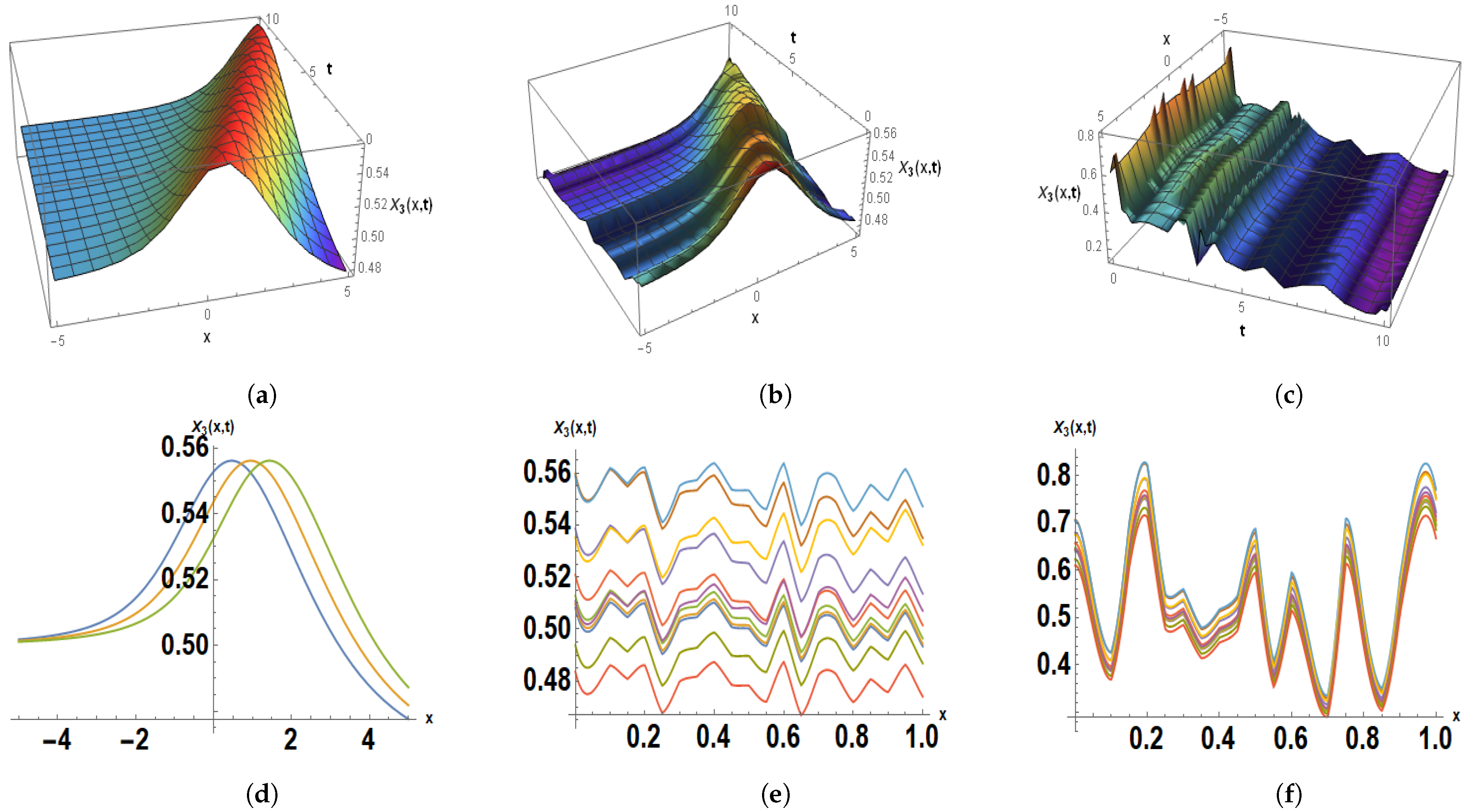
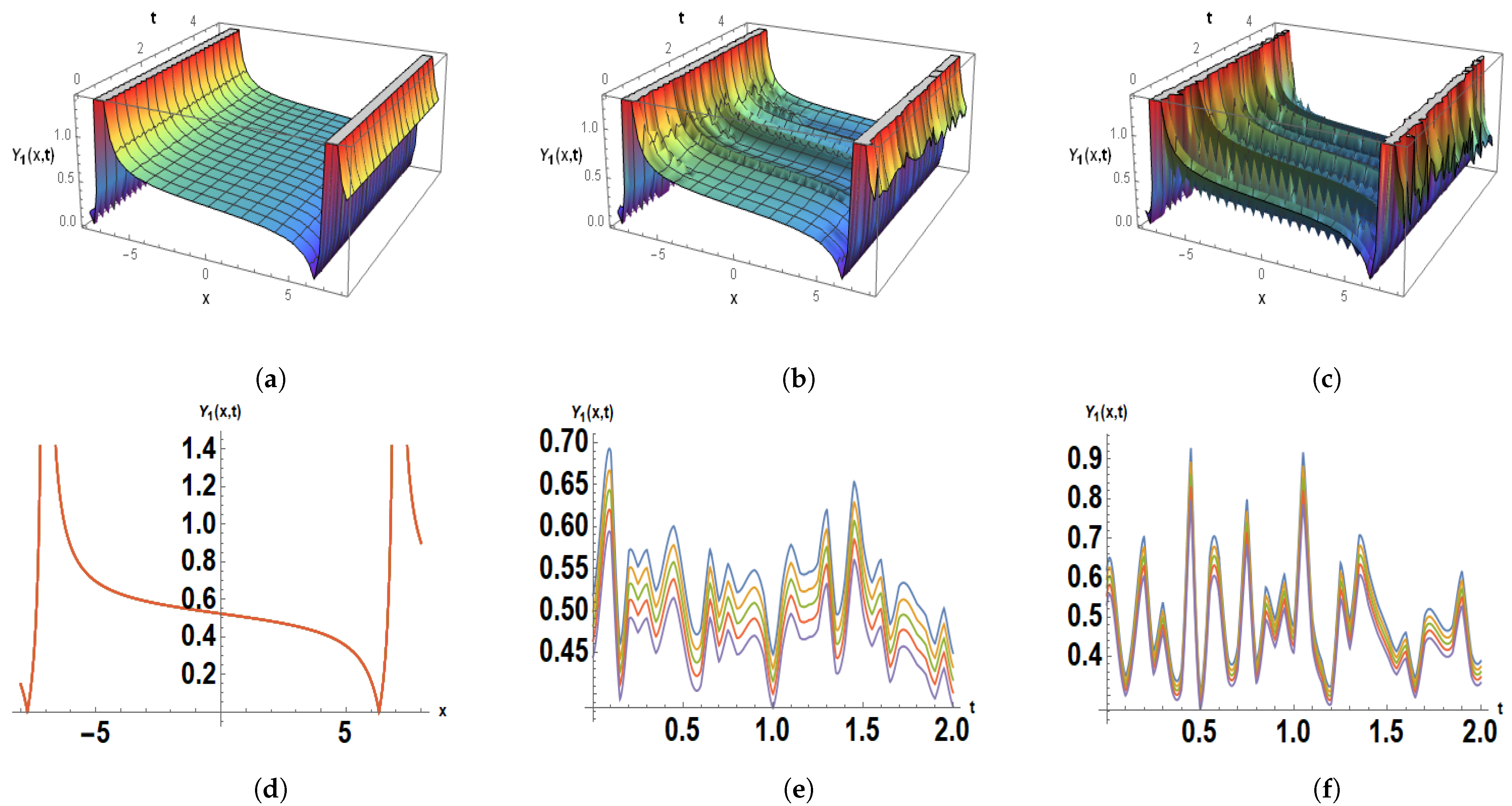
In this subsection, we discuss the physical behavior of the solitons and solitary wave solutions and their effects under noise. Solitons and solitary wave solutions can exhibit complex and diverse behavior when examining the biofilm model and quorum sensing in the context of noise. To completely understand this, one must consider both the mathematical features of the model and the biological impacts. Self-reinforcing, contained, stable waves that can maintain their shape and speed as they travel across a medium are referred to as solitons in mathematics. Solitons are commonly solitary wave solutions for some nonlinear partial differential equations (PDEs) that describe physical phenomena, such as biofilm formation under quorum sensing. The behavior of solitons and solitary waves can be greatly affected by the introduction of noise, either intrinsic or external. Random fluctuations or disturbances in the system can be used to mimic noise. Typically, stochastic partial differential equations (SPDEs) are used to study the impact of noise on solitons in PDEs. When choosing zero noise, these plots clearly demonstrate the right soliton shape.

Some solutions are presented in both 3D and 2D form for various values of the control parameter $\nu$. Figure 1 and Figure 4 provide us with the dark soliton. Figure 2 and Figure 5 give us the dark–bright soliton representations. Figure 3 and Figure 6 are plots for the solitary waves. Solitons can become unstable due to variations brought about by noise. Noise frequency and amplitude can affect how stable solitary wave solutions are.

The equilibrium between the intrinsic stability of the soliton and the intensity of the noise determines whether or not solitons persist in the presence of noise. Over time, noise can cause the soliton to spread out or lose its shape due to energy dissipation.

Diffusion processes generated by noise can characterize spreading behavior. Random disturbances or oscillations in the biofilm environment may interfere with soliton behavior.

There are several possible results from the interaction, such as the annihilation of existing solitons or the generation of new ones.

6.2. Comparison of Results

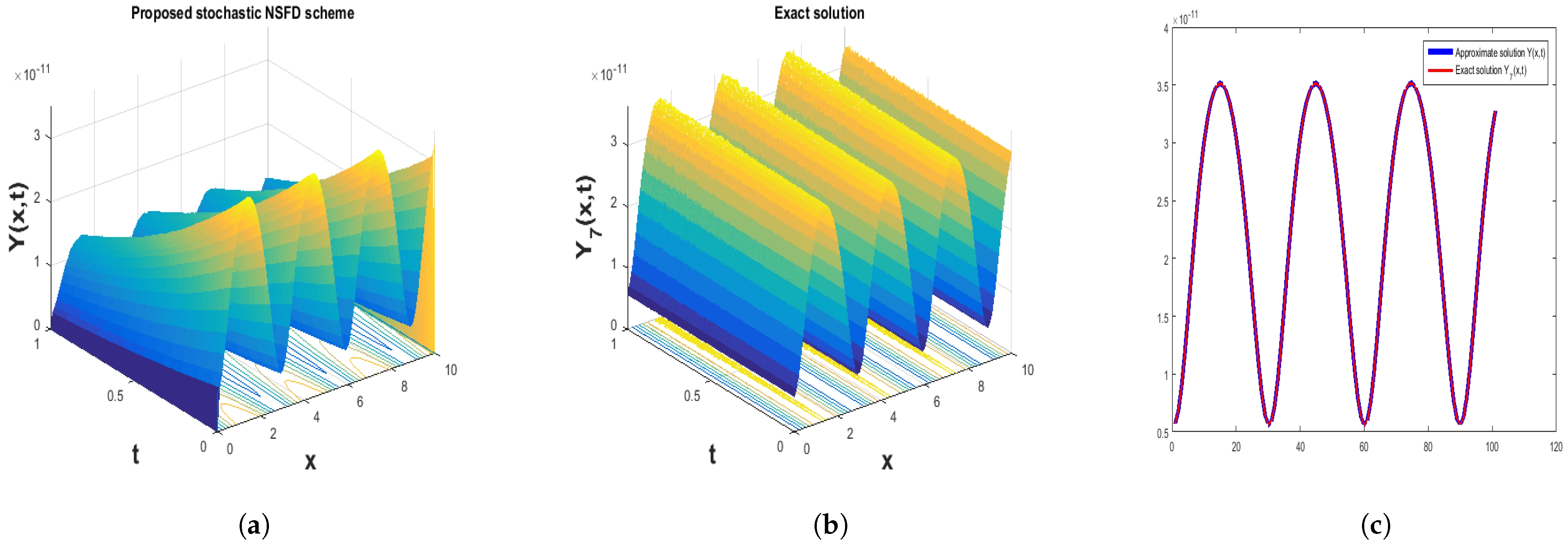
In this study, our main focus is to compare the numerical results with newly constructed exact solitary wave solutions. The proposed NSFD schemes are developed for the approximate solutions while generalized Riccati equation mapping is applied to gain the exact solitary wave solutions. Mainly, we compare the numerical result with selecting some exact solitary wave solutions. These results are visualized under the sense of noise, while we control the noise by ${\nu }_1$ and ${\nu }_2$. The motivation behind constructing initial conditions (ICs) and boundary conditions (BCs) for comparing numerical and solitary wave solutions in stochastic reaction–diffusion models lies in the desire to understand and analyze the behavior of complex systems accurately. Stochastic reaction–diffusion models are often used to simulate various biological, chemical, or physical phenomena. Validating these models is crucial for ensuring their accuracy in predicting real-world behavior. Constructing ICs and BCs provides a tangible platform for comparing the results obtained from numerical simulations with experimental observations, thereby validating the numerical models. Solitary waves, also known as solitons, are localized wave solutions that propagate without changing their shape. These waves are significant in various fields, including biology, physics, and engineering. By comparing numerical solutions with experimental observations obtained from ICs and BCs, researchers can gain insights into the dynamics of solitary waves in stochastic reaction–diffusion systems, helping to refine theoretical models and understand their implications in real systems. For the numerical experiment we always need ICs and BCs that are usually constructed by the exact solutions. In this study, we constructed them from the newly exact solitary wave solutions to compare the results. All the figures clearly show random behavior in their physical representation. The 3D and line plot show almost the same behavior for both numerical and exact solutions. These results are a very effective study of the biofilm dynamical model. This study is very fruitful for the further investigation of the dynamical model. When we deal with the results at the microlevel they show the randomness in their behavior.

Test Problem 1: To compare the graphical representation the proposed scheme (6) is considered for the approximate solutions while the exact solution, from (45) and the IC, is taken as

$$\begin{array}{c}\hfill Y(x,0)=0.000148105-0.000148105tanh\left(1.71828x\right).\end{array}$$

(97)

Figure 7 represents the 3D and line behavior for the proposed scheme (7) and exact solitary wave solution $Y_1(x,t)$ using the parameters values as $\zeta =1.1,\theta =3.5,\kappa =0.1,k=1$, ${\nu }_2=0.51,\xi =0.4,$ and $\sigma =0.0007$.

Test Problem 2: To compare the graphical representation the proposed NSFD scheme (6) is considered for the approximate solutions, while the exact solution from (47) and the IC is taken as

$$\begin{array}{c}\hfill X(x,0)=0.0100243+0.0015{((0.+2.92575i)\mathrm{sech}\left(2.92575x\right)+2.92575tanh\left(2.92575x\right)+3.)}^2,\end{array}$$

(98)

and the BCs are

$$\begin{array}{ccc}\hfill X(0,t)& =& 0.570003e^{-0.15t}\left(0.0100243+0.0015\left((0.+2.92575i)\mathrm{sech}\left(0.0441522t\right)\right.\right.\hfill \\ & & \left.{\left.-2.92575tanh\left(0.0441522t\right)+3\right)}^2\right),\hfill \end{array}$$

(99)

$$\begin{array}{ccc}\hfill X(10,t)& =& 0.570003e^{-0.15t}\left(0.0100243+0.0015(3+2.92575\left(tanh(29.2575-0.0441522t)\right.\right.\hfill \\ & & \left.{\left.+i\mathrm{sech}(29.2575-0.0441522t))\right)}^2\right).\hfill \end{array}$$

(100)

Figure 8 represents the 3D and line behavior for the proposed scheme (6) and the exact solitary wave solution $X_3(x,t)$ using the parameter values $\alpha =0.02,A=0.001$, $\beta =0.02$, $\gamma =0.01,\zeta =0.1,\theta =3,\kappa =1.1,k=1.0004,{\nu }_1=0.3,{\tau }_0=0.000982,$ and ${\tau }_1=0.02$.

Test Problem 3: To compare the graphical representation the proposed NSFD scheme (7) is considered for the approximate solutions while the exact solution from (48) and the IC is taken as

$$\begin{array}{c}\hfill Y(x,0)=-\left({7.976849408707993}^{-8}i\right)sech\left(2.92575x\right)-{7.976849408707993}^{-8}\\ \hfill tanh\left(2.92575x\right)+{7.976849408707992}^{-8}.\end{array}$$

(101)

Figure 9 represents the 3D and line behavior for the proposed scheme (7) and the exact solitary wave solution $Y_3(x,t)$ using the parameter values $\zeta =0.1,\theta =3,\kappa =1.1,k=1.0004,{\nu }_2=0.3,\xi =0.004,$ and $\sigma =0.00007$.

Test Problem 4: To compare the graphical representation the proposed NSFD scheme (6) is considered for the approximate solutions while the exact solution from (53) and the IC is taken as

$$\begin{array}{c}\hfill X(x,0)=1.43391\left(0.0015{\left(\frac{9.25203-8.77724cosh\left(2.92575x\right)}{3.sinh\left(2.92575x\right)+1.}-3\right)}^2+0.0100243\right),\end{array}$$

(102)

and the BCs are

$$\begin{array}{c}\hfill X(0,t)=1.43391e^{-0.15t}\left(0.0015{\left(\frac{9.25203-8.77724cosh\left(0.0441522t\right)}{1-3sinh\left(0.0441522t\right)}-3\right)}^2+0.0100243\right),\end{array}$$

(103)

$$\begin{array}{c}\hfill X(10,t)=\frac{e^{-0.15t}\left(5.81333\times {10}^{23}{e}^{-0.0883044t}-1.10721\times {10}^{11}{e}^{-0.0441522t}\right)}{{(1.sinh(29.2575-0.0441522t)+0.333333)}^2}.\end{array}$$

(104)

Figure 10 represents the 3D and line behavior for the proposed scheme (6) and the exact solitary wave solution $X_6(x,t)$ using the parameters $\alpha =0.02,A=0.001,\beta =0.02$, $\gamma =0.01,\zeta =0.1,\theta =3,\kappa =1.1,k=1.0004,{\nu }_1=0.3,{\tau }_0=0.000982,{\tau }_1=0.02,G=3,$ and $H=1$.

Test Problem 5: To compare the graphical representation the proposed NSFD scheme (7) is considered for the approximate solutions while the exact solution from (54) and the IC is taken as

$$\begin{array}{c}\hfill Y(x,0)=\frac{{5.0186952546034645}^{-20}i{e}^{(-1.22882i)x}+(-{2.8766831763675397}^{-36}-{6.963067713809684}^{-20}i)}{sin\left(1.22882x\right)+(-0.333333i)}.\end{array}$$

(105)

Figure 11 represents the 3D and line behavior for the proposed scheme (7) and the exact solitary wave solution $Y_6(x,t)$ using the parameters $\zeta =1,\theta =1.7,\kappa =1.1,k=0.4,{\nu }_2=0.3,\xi =4^{-10},\sigma =7^{-11},G=3,$ and $H=1$.

Test Problem 6: To compare the graphical representation the proposed NSFD scheme (6) is considered for the approximate solutions while the exact solution from (55) and the IC is taken as

$$\begin{array}{c}\hfill X(x,0)=1.01411\left(1.20888+0.045{\left(-1.7+\frac{1.11056-1.05357cos\left(1.05357x\right)}{1.sin\left(1.05357x\right)+(0.-0.333333i)}\right)}^2\right),\end{array}$$

(106)

and the BCs are

$$\begin{array}{ccc}\hfill X(0,t)& =& 1.01411e^{-0.15t}\left(1.20888+0.045{\left(-1.7+\frac{1.05357cos\left(0.0897216t\right)-1.11056}{1.sin\left(0.0897216t\right)+(0.+0.333333i)}\right)}^2\right),\hfill \end{array}$$

(107)

$$\begin{array}{ccc}\hfill X(10,t)& =& 1.01411e^{-0.15t}\left(1.20888\right.\hfill \\ & & \left.+\frac{0.178384{((0.557787+0.284614i)+0.0951763sin\left(0.0897216t\right)+1.cos\left(0.0897216t\right))}^2}{{(-1.sin(10.5357-0.0897216t)+(0.+0.333333i))}^2}\right).\hfill \end{array}$$

(108)

Figure 12 represents the 3D and line behavior for the proposed scheme (6) and the exact solitary wave solution $X_7(x,t)$ using the parameters $\alpha =0.4,A=0.01,\beta =1.2$, $\gamma =0.001,\zeta =1,\theta =1.7,\kappa =1,{\nu }_1=0.3,G=3,H=1,{\tau }_0=0.982,{\tau }_1=0.32$.

Test Problem 7: To compare the graphical representation the proposed NSFD scheme (7) is considered for the approximate solutions while the exact solution from (54) and the IC is taken as

$$\begin{array}{ccc}\hfill Y(x,0)& =& \left(\left({3.5493768697990816}^{-11}i\right)cos\left(1.05357x\right)+({3.5493768697990816}^{-11}-{8.738023015898668}^{-27}i)\right.\hfill \\ & & \left.sin\left(1.05357x\right)+({3.346384604828817}^{-11}-{1.1831256232663607}^{-11}i)\right)\hfill \\ & & /\left(sin\left(1.05357x\right)+(-0.333333i)\right).\hfill \end{array}$$

(109)

Figure 13 represents the 3D and line behavior for the proposed scheme (7) and the exact solitary wave solution $Y_7(x,t)$ using the parameters $\zeta =1,\theta =1.7,\kappa =1,k=0.4,{\nu }_2=0.3,\xi =0.4,\sigma =7^{-11},G=3$ and $H=1$.

Test Problem 8: To compare the graphical representation the proposed NSFD scheme (6) is considered for the approximate solutions while the exact solution from (77) and the IC is taken as

$$\begin{array}{ccc}\hfill X(x,0)& =& 0.880037\left(1.21774\right.\hfill \\ & & \left.+\frac{0.28755{((2.01753-2.82843i)+0.67251sin\left(2.52784x\right)+1.cos\left(2.52784x\right))}^2}{{(sin\left(2.52784x\right)+3.)}^2}\right),\hfill \end{array}$$

(110)

and the BCs are

$$\begin{array}{ccc}\hfill X(0,t)& =& 0.880037e^{-0.05t}\left(1.21774\right.\hfill \\ & & \left.+0.045{\left(-1.7+\frac{2.52784cos\left(0.0214867t\right)+(0.-7.14983i)}{sin\left(0.0214867t\right)-3.}\right)}^2\right),\hfill \end{array}$$

(111)

$$\begin{array}{ccc}\hfill X(10,t)& =& 0.880037e^{-0.05t}\left(1.21774\right.\hfill \\ & & \left.+0.045{\left(-1.7+\frac{-2.52784cos(25.2784-0.0214867t)+(0.+7.14983i)}{sin(25.2784-0.0214867t)+3.}\right)}^2\right).\hfill \end{array}$$

(112)

Figure 14 represents the 3D and line behavior for the proposed scheme (6) and the exact solitary wave solution $X_{18}(x,t)$ using the parameter values $\alpha =0.04,A=0.001$, $\beta =1.2$, $\gamma =0.001,\zeta =2.9,\theta =1.7,\kappa =0.8,{\nu }_1=0.1,{\tau }_0={9.82}^{-8},{\tau }_1={3.2}^{-9},G=1$ and $H=3$.

7. Conclusions

In this article, we investigated the stochastic reaction–diffusion biofilm model under the randomness effect numerically and analytically. The two outcomes of this model are the concentration of bacteria, which over time depicts the development and decomposition of the biofilm, and the collaboration of the bacteria in the biofilm, which shows the efficacy of resistance and defense against environmental stimuli.

The suggested finite difference scheme performs the numerical solutions. Visualizations of the scheme’s analysis include stability and consistency. Mean square sense is used to evaluate the consistency of the scheme, while the Von Neumann criteria are used to determine stability. Additionally, the generalized Riccati equation mapping approach is used to derive stochastic exact solitary wave solutions in trigonometric, hyperbolic, and rational forms. Some solutions are drawn in 3D and 2D to show the different soliton behavior and their effects on noise. These plots show that if we choose noise strength zero these solutions give us the proper soliton solutions and how noise affects them when we increase the value of $\nu$. Mainly, the numerical results are compared with the exact solitary wave solutions with the help of unique physical problems. The comparison plots are presented in 3D and line representations as well by selecting different values of the parameters.

References

1. Grzybowski, B.A. Chemistry in Motion: Reaction-Diffusion Systems for Micro-and Nanotechnology; John Wiley & Sons: Hoboken, NJ, USA, 2009. [Google Scholar]
2. Wu, Y.F. Computational Systems Analysis of Deterministic Pair Rule Gene Network and Stochastic Bicoid Morphogen Gradient in Drosophila Melanogaster. Ph.D. Thesis, State University of New York at Stony Brook, New York, NY, USA, 2011. [Google Scholar]
3. Iqbal, M.S.; Baber, M.Z.; Inc, M.; Younis, M.; Ahmed, N.; Qasim, M. On multiple solitons of glycolysis reaction–diffusion system for the chemical concentration. Int. J. Mod. Phys. B 2023, 38, 2450055. [Google Scholar] [CrossRef]
4. Shi, S.; Han, D.; Cui, M. A multimodal hybrid parallel network intrusion detection model. Connect. Sci. 2023, 35, 2227780. [Google Scholar] [CrossRef]
5. Wang, J.; Xu, Z.; Zheng, X.; Liu, Z. A fuzzy logic path planning algorithm based on geometric landmarks and kinetic constraints. Inf. Technol. Control 2022, 51, 499–514. [Google Scholar] [CrossRef]
6. Zhang, X.; Feng, Z.; Zhang, X. On reachable set problem for impulse switched singular systems with mixed delays. IET Control Theory Appl. 2023, 17, 628–638. [Google Scholar] [CrossRef]
7. Zou, Z.; Guo, R. The Riemann–Hilbert approach for the higher-order Gerdjikov–Ivanov equation, soliton interactions and position shift. Commun. Nonlinear Sci. Numer. Simul. 2023, 124, 107316. [Google Scholar] [CrossRef]
8. Solhi, E.; Mirzaee, F.; Naserifar, S. Enhanced moving least squares method for solving the stochastic fractional Volterra integro-differential equations of Hammerstein type. Numer. Algorithms 2023, 95, 1921–1951. [Google Scholar] [CrossRef]
9. Waters, C.M.; Bassler, B.L. Quorum sensing: Cell-to-cell communication in bacteria. Annu. Rev. Cell Dev. Biol. 2005, 21, 319–346. [Google Scholar] [CrossRef]
10. Banasiak, J.; Mokhtar-Kharroubi, M. (Eds.) Evolutionary Equations with Applications in Natural Sciences; Lecture Notes in Mathematics 2126; Springer: Berlin/Heidelberg, Germany, 2015. [Google Scholar]
11. Baber, M.Z.; Seadawy, A.R.; Iqbal, M.S.; Rizvi, S.T. Optimization and exact solutions for biofilm model of bacterial communities. Alex. Eng. J. 2024, 90, 89–97. [Google Scholar] [CrossRef]
12. Taghizadeh, L.; Karimi, A.; Presterl, E.; Heitzinger, C. Bayesian inversion for a biofilm model including quorum sensing. Comput. Biol. Med. 2020, 117, 103582. [Google Scholar] [CrossRef]
13. Yasin, M.W.; Iqbal, M.S.; Ahmed, N.; Akgül, A.; Raza, A.; Rafiq, M.; Riaz, M.B. Numerical scheme and stability analysis of stochastic Fitzhugh–Nagumo model. Results Phys. 2022, 32, 105023. [Google Scholar] [CrossRef]
14. Baber, M.Z.; Seadway, A.R.; Ahmed, N.; Iqbal, M.S.; Yasin, M.W. Selection of solitons coinciding the numerical solutions for uniquely solvable physical problems: A comparative study for the nonlinear stochastic Gross–Pitaevskii equation in dispersive media. Int. J. Mod. Phys. B 2022, 37, 2350191. [Google Scholar] [CrossRef]
15. Ahmed, N.; Yasin, M.W.; Iqbal, M.S.; Raza, A.; Rafiq, M.; Inc, M. A dynamical study on stochastic reaction diffusion epidemic model with nonlinear incidence rate. Eur. Phys. J. Plus 2023, 138, 350. [Google Scholar] [CrossRef] [PubMed]
16. Cannon, J.R.; Yanping, L.; Shingmin, W. An implicit finite difference scheme for the diffusion equation subject to mass specification. Int. J. Eng. Sci. 1990, 28, 573–578. [Google Scholar] [CrossRef]
17. Yasin, M.W.; Ahmed, N.; Iqbal, M.S.; Rafiq, M.; Raza, A.; Akgül, A. Reliable numerical analysis for stochastic reaction-diffusion system. Phys. Scr. 2022, 98, 015209. [Google Scholar] [CrossRef]
18. Iqbal, M.S.; Seadawy, A.R.; Baber, M.Z. Demonstration of unique problems from Soliton solutions to nonlinear Selkov–Schnakenberg system. Chaos Solitons Fractals 2022, 162, 112485. [Google Scholar] [CrossRef]
19. Younis, M.; Seadawy, A.R.; Baber, M.Z.; Husain, S.; Iqbal, M.S.; Rizvi, S.T.R.; Baleanu, D. Analytical optical soliton solutions of the Schrödinger-Poisson dynamical system. Results Phys. 2021, 27, 104369. [Google Scholar] [CrossRef]
20. Naher, H.; Abdullah, F.A. The modified Benjamin-Bona-Mahony equation via the extended generalized Riccati equation mapping method. Appl. Math. Sci. 2012, 6, 5495–5512. [Google Scholar]
21. Zhu, S.D. The generalizing Riccati equation mapping method in non-linear evolution equation: Application to (2+1)-dimensional Boiti–Leon–Pempinelle equation. Chaos Solitons Fractals 2008, 37, 1335–1342. [Google Scholar] [CrossRef]
22. Iqbal, M.S.; Seadawy, A.R.; Baber, M.Z.; Ahmed, N.; Yasin, M.W. Extraction of solitons for time incapable illimitable paraxial wave equation in Kerr-media. Int. J. Mod. Phys. B 2022, 37, 2350122. [Google Scholar] [CrossRef]
23. Iqbal, M.S.; Seadawy, A.R.; Baber, M.Z.; Qasim, M. Application of modified exponential rational function method to Jaulent–Miodek system leading to exact classical solutions. Chaos Solitons Fractals 2022, 164, 112600. [Google Scholar] [CrossRef]
24. Zhao, Y.H.; Iqbal, M.S.; Baber, M.Z.; Inc, M.; Ahmed, M.O.; Khurshid, H. On traveling wave solutions of an autocatalytic reaction–diffusion Selkov–Schnakenberg system. Results Phys. 2023, 44, 106129. [Google Scholar] [CrossRef]
25. Mohammed, W.W.; El-Morshedy, M.; Cesarano, C.; Al-Askar, F.M. Soliton solutions of fractional stochastic Kraenkel–Manna–Merle equations in ferromagnetic materials. Fractal Fract. 2023, 7, 328. [Google Scholar] [CrossRef]
26. Mohammed, W.W.; Iqbal, N.; Ali, A.; El-Morshedy, M. Exact solutions of the stochastic new coupled Konno-Oono equation. Results Phys. 2021, 21, 103830. [Google Scholar] [CrossRef]
27. Baber, M.Z.; Ahmed, N.; Yasin, M.W.; Iqbal, M.S.; Akgül, A.; Riaz, M.B.; Rafiq, M.; Raza, A. Comparative analysis of numerical with optical soliton solutions of stochastic Gross–Pitaevskii equation in dispersive media. Results Phys. 2023, 44, 106175. [Google Scholar] [CrossRef]
28. Guo, S.; Mei, L.; Zhou, Y.; Li, C. The extended Riccati equation mapping method for variable-coefficient diffusion–reaction and mKdV equations. Appl. Math. Comput. 2011, 217, 6264–6272. [Google Scholar] [CrossRef]
29. Younis, M.; Seadawy, A.R.; Sikandar, I.; Baber, M.Z.; Ahmed, N.; Rizvi, S.T.R.; Althobaiti, S. Nonlinear dynamical study to time fractional Dullian–Gottwald–Holm model of shallow water waves. Int. J. Mod. Phys. B 2022, 36, 2250004. [Google Scholar] [CrossRef]
30. Shaikh, T.S.; Baber, M.Z.; Ahmed, N.; Shahid, N.; Akgül, A.; De la Sen, M. On the Soliton Solutions for the Stochastic Konno–Oono System in Magnetic Field with the Presence of Noise. Mathematics 2023, 11, 1472. [Google Scholar] [CrossRef]
31. Al-Askar, F.M.; Cesarano, C.; Mohammed, W.W. The Influence of White Noise and the Beta Derivative on the Solutions of the BBM Equation. Axioms 2023, 12, 447. [Google Scholar] [CrossRef]
Figure 1. Dark soliton for the solution X 1 ( x , t ) and its different effects of noise: (a) 3D plot when ν = 0 . (b) 3D plot when ν = 0.3 . (c) 3D plot when ν = 0.5 . (d) 2D plot when ν = 0 . (e) 2D plot when ν = 0.3 . (f) 2D plot when ν = 0.5 .
Mathematics 12 01293 g001
Figure 2. Dark–bright soliton for the solution X 3 ( x , t ) and its different effects of noise: (a) 3D plot when ν = 0 . (b) 3D plot when ν = 0.1 . (c) 3D plot when ν = 0.5 . (d) 2D plot when ν = 0 . (e) 2D plot when ν = 0.1 ; (f) 2D plot when ν = 0.5 .
Mathematics 12 01293 g002
Figure 3. Solitary wave solution for the solution X 18 ( x , t ) and its different effects of noise: (a) 3D plot when ν = 0 . (b) 3D plot when ν = 0.3 . (c) 3D plot when ν = 0.5 . (d) 2D plot when ν = 0 . (e) 2D plot when ν = 0.3 . (f) 2D plot when ν = 0.5 .
Mathematics 12 01293 g003
Figure 4. Dark soliton for the solution Y 1 ( x , t ) and its different effects of noise: (a) 3D plot when ν = 0 . (b) 3D plot when ν = 0.3 . (c) 3D plot when ν = 0.5 ; (d) 2D plot when ν = 0 . (e) 2D plot when ν = 0.3 . (f) 2D plot when ν = 0.5 .
Mathematics 12 01293 g004
Figure 5. Dark soliton for the solution Y 3 ( x , t ) and its different effects of noise: (a) 3D plot when ν = 0 . (b) 3D plot when ν = 0.3 . (c) 3D plot when ν = 0.5 . (d) 2D plot when ν = 0 . (e) 2D plot when ν = 0.3 . (f) 2D plot when ν = 0.5 .
Mathematics 12 01293 g005
Figure 6. Solitary wave for the solution Y 18 ( x , t ) and its different effects of noise: (a) 3D plot when ν = 0 . (b) 3D plot when ν = 0.3 . (c) 3D plot when ν = 0.5 ; (d) 2D plot when ν = 0 . (e) 2D plot when ν = 0.3 . (f) 2D plot when ν = 0.5 .
Mathematics 12 01293 g006
Figure 7. Comparison of results in 3D and line plots for Test 1: (a) Proposed scheme Y(x,t). (b) Exact solution Y 1 ( x , t ) . (c) Line graph of both solutions.
Mathematics 12 01293 g007
Figure 8. Comparison of results in 3D and line plots for Test 2: (a) Proposed NSFD scheme X(x,t). (b) Exact solution X 3 ( x , t ) . (c) Line graph of both solutions.
Mathematics 12 01293 g008
Figure 9. Comparison of results in 3D and line plots for Test 3: (a) Proposed scheme Y(x,t). (b) Exact solution Y 3 ( x , t ) . (c) Line graph of both solutions.
Mathematics 12 01293 g009
Figure 10. Comparison of results in 3D and line plots for Test 4: (a) Proposed scheme Y(x,t). (b) Exact solution X 6 ( x , t ) . (c) Line graph of both solutions.
Mathematics 12 01293 g010
Figure 11. Comparison of results in 3D and line plots for Test 5: (a) Proposed scheme Y(x,t). (b) Exact solution Y 6 ( x , t ) . (c) Line graph of both solutions.
Mathematics 12 01293 g011
Figure 12. Comparison of results in 3D and line plots for Test 6: (a) Proposed scheme Y(x,t). (b) Exact solution X 7 ( x , t ) . (c) Line graph of both solutions.
Mathematics 12 01293 g012
Figure 13. Comparison of results in 3D and line plots for Test 7: (a) Proposed scheme Y(x,t). (b) Exact solution Y 7 ( x , t ) . (c) Line graph of both solutions.
Mathematics 12 01293 g013
Figure 14. Comparison of results in 3D and line plots for Test 8: (a) Proposed scheme Y(x,t). (b) Exact solution X 18 ( x , t ) . (c) Line graph of both solutions.
Mathematics 12 01293 g014
Disclaimer/Publisher’s Note: The statements, opinions and data contained in all publications are solely those of the individual author(s) and contributor(s) and not of MDPI and/or the editor(s). MDPI and/or the editor(s) disclaim responsibility for any injury to people or property resulting from any ideas, methods, instructions or products referred to in the content.