Abstract
Survival analysis is a fundamental tool for modeling time-to-event data in healthcare, engineering, and finance, where censored observations pose significant challenges. While traditional methods like the Beran estimator offer nonparametric solutions, they often struggle with the complex data structures and heavy censoring. This paper introduces three novel survival models, iSurvM (imprecise Survival model based on Mean likelihood functions), iSurvQ (imprecise Survival model based on Quantiles of likelihood functions), and iSurvJ (imprecise Survival model based on Joint learning), that combine imprecise probability theory with attention mechanisms to handle censored data without parametric assumptions. The first idea behind the models is to represent censored observations by interval-valued probability distributions for each instance over time intervals between event moments. The second idea is to employ the kernel-based Nadaraya–Watson regression with trainable attention weights for computing the imprecise probability distribution over time intervals for the entire dataset. The third idea is to consider three decision strategies for training, which correspond to the proposed three models. Experiments on synthetic and real datasets demonstrate that the proposed models, especially iSurvJ, consistently outperform the Beran estimator from accuracy and computational complexity points of view. Codes implementing the proposed models are publicly available.
Keywords:
survival analysis; censored data; classification; attention mechanism; imprecise probabilities; Beran estimator MSC:
68T07; 62N02
1. Introduction
Survival analysis [1], or time-to-event analysis, provides a robust framework for modeling time-to-event data across diverse domains. In healthcare, it predicts critical outcomes such as mortality, disease recurrence, and recovery timelines while quantifying treatment effectiveness and disease progression. In engineering, the method assesses reliability, predicting system failures, optimizing maintenance schedules, and evaluating product durability. It also proves valuable in financial risk modeling (e.g., credit defaults and customer churn) and industrial contexts (e.g., equipment degradation and failure prediction). A key strength of survival analysis is its ability to handle censored data, making it indispensable for scenarios with incomplete event observations, from clinical trials to mechanical system monitoring. This approach delivers quantifiable insights into event timing uncertainty across these fields.
Due to the importance of tasks addressed by survival analysis, numerous machine learning models have been developed to handle time-to-event data and solve related problems within this framework [2,3,4,5,6,7,8]. Comprehensive reviews of these models are available in [9,10,11].
Many of these models adapt and extend traditional classification and regression techniques to handle the unique challenges of survival analysis, for example, random survival forests [12], survival support vector machines [13], neural networks [14], and survival-oriented transformers [15,16,17,18]. These methods demonstrate the growing intersection of classical survival analysis with modern machine learning paradigms.
Survival analysis often involves modeling time-to-event data in the presence of covariates or feature vectors. While traditional nonparametric methods like the Kaplan–Meier estimator [19] assume independence between survival times and covariates, conditional survival models incorporate covariate information to provide more personalized estimates. A prominent example is the Beran estimator [20], a nonparametric conditional survival function estimator that extends the Kaplan–Meier approach by incorporating kernel weighting based on covariates. Kernel-based methods, like the Beran estimator, provide flexible, nonparametric approaches to survival analysis by leveraging smoothing techniques to model time-to-event data with covariates. They offer a powerful toolkit for survival analysis, especially when parametric assumptions fail. Chen [21] presented a neural network framework based on kernels. The deep kernel conditional Kaplan–Meier estimator was introduced in [21]. Sparse kernel methods based on applying SVM were considered in [22]. Instead of estimating the survival function directly, some approaches smooth the cumulative hazard function [23]. A series of survival models based on applying Bayesian kernel methods which combine the flexibility of kernel-based nonparametric modeling with the probabilistic rigor of Bayesian inference [24]. Another kernel-based method is the kernel Cox regression [25,26,27] which relaxes the assumption of the linear covariate effects accepted in the original Cox model [28] by allowing nonlinear effects via kernel functions.
Survival analysis is traditionally framed as a time-to-event prediction problem, but it can also be approached as a classification task by discretizing time and predicting event probabilities over intervals in the framework of discrete-time survival analysis [29], where continuous survival data can be converted into a person–period format [30]. The loss functions in this case are based on applying the likelihood function [31]. A method for treating survival analysis as a classification problem was proposed in [32] where a “stacking” idea was used to collect features and outcomes of the survival data in a large data frame and then to solve the classification problem.
We propose a novel approach within the framework of discrete-time survival analysis, which can be characterized as imprecise survival modeling. The core idea is to model non-parametric probability distributions over time intervals for each instance in the training set. For uncensored observations, the distribution is degenerate, where the event’s true time interval has probability one while all others have probability zero. For censored observations, the probability of the event occurring in any interval after the censored time can range from zero to one, reflecting prior ignorance. This introduces imprecision, meaning each instance induces a set of possible probability distributions. To aggregate the probability distributions generated for each instance from the training set, we propose to employ kernel Nadaraya–Watson regression [33,34] with trainable dot-product attention weights [35,36]. We propose three training strategies, each leading to a distinct model. The first two strategies are based on generating random probability distributions from the produced sets of distributions. The first strategy averages all loss functions in the form of the likelihood function in accordance with the aggregated probability distributions. The corresponding model is called iSurvM (imprecise Survival model based on Mean likelihood functions). The second strategy averages only a portion of the largest values of the loss functions over the generated probability distributions. The corresponding model is called iSurvQ (imprecise Survival model based on Quantiles of likelihood functions). According to the third strategy, the probability distributions and the attention weights are jointly learned in a special way without using the generation procedure. The corresponding model is called iSurvJ (imprecise Survival model based on Joint learning). We avoid any assumptions associated with a survival model, for example, the Cox model, which define the loss functions for training the models (see, for example, [37]).
In contrast to many imprecise models for survival analysis [38,39,40], the proposed models do not consider the incomplete or partial knowledge in event time data. They represent censored observations as interval-valued or imprecise data.
Our contributions can be summarized as follows:
- We propose three training strategies and the corresponding survival models, iSurvM, iSurvQ, iSurvJ, as an alternative to kernel-based models such as the Beran estimator.
- The models can be trained using different attention mechanisms implemented by means of neural networks as well as simple Gaussian kernels (an additional model iSurvJ(G) which uses a Gaussian kernel for the attention weights). The number of trainable parameters depends on the key and query attention matrices and can be arbitrarily chosen.
- Additionally, unlike Beran estimators, the proposed models impose no restrictions on the number of concurrent event times, making them more versatile. Moreover, a high proportion of censored data does not lead to significant accuracy degradation in the proposed models, unlike in Beran estimators.
- No parametric assumptions are made in the proposed models.
- Various numerical experiments with real and synthetic datasets are conducted to compare the proposed survival models with each other under different conditions and to compare them with the Beran estimator using the concordance index and the Brier score. We compare the proposed models with the Beran estimator, but not with available transformer-based models [16,41,42], because the introduced models are regarded as alternatives to the kernel-based Beran estimator and can be incorporated into a more complex model as a component. The corresponding codes implementing the proposed models are publicly available at: https://github.com/NTAILab/iSurvMQJ (accessed on 14 September 2025).
The paper is organized as follows. Related work devoted to machine learning models in survival analysis, to kernel-based methods and models in survival analysis, and to imprecise models in survival analysis can be found in Section 2. Section 3 provides basic definitions of survival analysis, the attention mechanism, and the Nadaraya–Watson regression. Survival analysis as an imprecise multi-label classification problem is considered in Section 4. Training strategies and survival models iSurvM, iSurvQ, iSurvJ are studied in Section 5. Numerical experiments with well-known public real and synthetic data illustrating the proposed models are given in Section 6. Concluding remarks are provided in Section 7.
2. Related Work
Machine learning models in survival analysis. Survival analysis, which deals with time-to-event data, has seen significant advancements through the integration of machine learning techniques. Numerous models have been developed to predict survival times, hazard functions, and other key measures, leveraging both traditional statistical methods and modern computational approaches. Several comprehensive reviews and surveys provide detailed insights into these developments. For instance, ref. [10] offers a broad examination of machine learning methods in survival analysis, while [9] and [43] discuss recent trends, including deep learning and high-dimensional data applications. Additionally, ref. [44] provides a methodological perspective on generalizing survival models, and [45] explores interpretability and benchmarking in survival machine learning. A more contemporary discussion on emerging techniques and challenges in the field can be found in [11].
Kernel-based methods and models in survival analysis. An important kernel-based approach to survival analysis is the Beran estimator [20], which extends the Kaplan–Meier estimator by incorporating covariate information through kernel smoothing. The Beran estimator or the conditional Kaplan–Meier estimator [46] enables robust estimation of survival functions in complex, high-dimensional settings. Recent advances have further enhanced these techniques through integration with deep learning. For instance, ref. [21] proposed a neural network framework that automatically learned optimal kernel functions for survival analysis, leading to the development of the deep kernel conditional Kaplan–Meier estimator, which improved adaptability to heterogeneous data structures.
Alternative kernel-based strategies include sparse kernel methods via support vector machines (SVMs) [22], which enhance computational efficiency, and approaches that focus on smoothing the cumulative hazard function rather than the survival function directly [23]. Bayesian formulations of kernel methods, such as those in [24], combine the flexibility of nonparametric modeling with the probabilistic rigor of Bayesian inference, offering uncertainty quantification alongside predictive accuracy.
Another significant direction is the kernel Cox regression [25,26,27], which generalizes the classical Cox model [28] by replacing linear covariate effects with nonlinear kernel-based relationships. This relaxation captures intricate dependencies in the data, addressing a key limitation of the original proportional hazards framework. Collectively, these methods demonstrate the versatility of kernel-based techniques in survival analysis, balancing interpretability, computational tractability, and adaptability to diverse data regimes.
Attention mechanism. Recent advances in survival analysis have leveraged attention mechanisms [36] to improve interpretability and predictive accuracy. Deep learning approaches use attention to model complex, nonlinear relationships. The corresponding methods address key challenges like censoring, competing risks, and non-proportional hazards while providing interpretable feature importance. The attention mechanism was applied to different deep learning survival models. In particular, a self-attention mechanism was used to model local and global context simultaneously for survival analysis in [47]. The attention mechanism can be a part of transformers, which capture long-range dependencies in survival data, offering improved performance in high-dimensional settings. Transformers for survival analysis with competing events were proposed in [48]. Transformers solving survival machine learning problems were also proposed in [16,41,42]. Different applications of transformers to medical problems in the framework of survival analysis can be found in [49,50,51,52].
Imprecise models in survival analysis. It should be noted that the imprecise survival analysis extends classical survival models to account for partial or incomplete knowledge in time-to-event data. Unlike traditional methods that assume precise probabilities, imprecise models incorporate set-valued or interval-based estimates to reflect epistemic uncertainty, ambiguity in censoring mechanisms, or conflicting expert opinions. A method of statistical inference based on the Hill model [53] for data that include right-censored observations was proposed in [39], where the authors derive bounds for the predictive survival function. Another method of statistical inference based on the imprecise Dirichlet model [54] was proposed in [38]. A method applying a robust Dirichlet process for estimating survival functions from samples with right-censored data was introduced in [40]. It should be note that the proposed imprecise models cope with cases when exact event times are unknown or are interval-valued and strong distributional assumptions are violated.
3. Preliminaries
3.1. Survival Analysis
Datasets in survival analysis are represented by a set . Here, the vector consisting of d features characterizes the ith object. The time corresponds to one of two types of event observations. The first type is when the event is observed. In this case, the observation is called uncensored and the censoring indicator is equal to one. The second type is when the event is not observed, it is greater than , but its ‘true’ value is unknown. In this case, the observation is called censored and the censoring indicator is equal to zero. A survival model is trained on the set to predict probabilistic measures of an event time T for a new object represented by the vector x.
An important concept in survival analysis is the survival function (SF) . It is a function of time t defined as the probability of surviving up to time t, i.e., .
Many survival machine learning models have been developed in the last decades. In order to compare the models, special measures are used, different from the standard accuracy measures accepted in machine learning classification and regression models. The most popular measure in survival analysis is Harrell’s C-index (concordance index) [55]. It estimates the probability that, in a randomly selected pair of objects, the object that fails first had a worst predicted outcome. In fact, this is the probability that the event times of a pair of objects are correctly ranked. The C-index does not depend on choosing a fixed time for evaluation of the model and takes into account censoring of patients [56].
Let be a set of all pairs satisfying conditions and . The C-index is formally computed as proposed in [10,57]:
where and are predicted expected event times.
If the C-index is equal to one, then the corresponding survival model is supposed to be perfect. If the C-index is 0.5, then the model is not better than random guessing.
Another index used to compare survival models is the Brier Score (BS) [58,59] which is defined as
where is the true status of a new test subject, and is the predicted survival probability.
The Integrated Brier Score (IBS) extends the BS by averaging it over a range of time points, typically from to a maximum time . It is defined as:
3.2. Attention Mechanism and the Nadaraya–Watson Regression
The idea of the attention mechanism can be clearly illustrated using the Nadaraya–Watson kernel regression model [33,34]. Consider a training set with N instances, where each is a feature vector and is its corresponding label. For a new input feature vector , the regression output prediction can be estimated as a weighted average using the Nadaraya–Watson kernel regression model [33,34]:
Here, represents the attention weight with trainable parameters , which quantifies the similarity (or distance) between the input feature vector and the training feature vector . The closer is to , the larger the corresponding weight becomes. In general, any distance or similarity function satisfying this monotonicity condition can serve as attention weights. A natural choice is the family of kernel functions, since a kernel K inherently acts as a similarity measure between vectors and . Therefore, the attention weights can be expressed as:
In the context of the attention mechanism [60], the vector is referred to as the query, while vectors and labels are called the keys and values, respectively. The attention weights can be generalized by introducing trainable parameters. For example, using a Gaussian kernel with trainable parameter vector , the attention weight can be expressed as:
where is the softmax function.
Several definitions of attention weights and corresponding attention mechanisms exist in the literature. Notable examples include the additive attention [60] and multiplicative or dot-product attention [35,36].
4. Survival Analysis as an Imprecise Multi-Label Classification Problem
This section demonstrates how survival models can be formulated using the Nadaraya–Watson kernel regression.
Consider a partition of the time axis into discrete intervals:
such that
The partition divides the time axis into T intervals denoted as for . We assume that at each time point (or within interval ), there are uncensored events and right-censored events such that the total number of events is .
Let us define the probability that an event corresponding to the ith object is observed in the interval . This generates a probability distribution for each subject , . If the corresponding observation is uncensored, then the following holds:
For censored observations, the true event time must occur in some interval after , though the specific interval remains unknown. Consequently, the probability that the event is in each interval after time can be from zero to one, i.e.,
The interval is a form of prior ignorance. In all cases, we have the constraint for precise probabilities. However, this condition is not fulfilled when the upper or lower probabilities are summed. Due to imprecision of probabilities , we assume that the ith instance produces a set of probability distributions denoted as .
Let us consider the following classification problem. There is a set of feature vectors . The kth interval can be viewed as the kth class represented by the vector . Then, the Nadaraya–Watson kernel regression can be applied to find the class probability distribution of a new instance . Since the probabilities are interval values, then it is obvious that the predicted class probabilities are also interval values. They are determined as follows:
where is an attention weight expressed through kernels (see (5)), ; is the trainable vector of parameters.
The attention weights satisfy the condition
5. Training Strategies and Three Survival Models
5.1. A General Form of Attention Weights
Before presenting the proposed survival models, their common elements in terms of attention weights and regularization are described. We consider the attention weights in a general form. Let represent the matrix of the input keys (the matrix of N feature vectors , , from the training set), and represent the matrix of the input queries (the matrix of the same feature vectors from the training set). Here, is the dimension of the initial feature vectors , . The matrix is used in the training phase. In many tasks, the sparse representation of feature vectors might be useful. In order to implement it, matrices and can be transformed to sets of vectors of a new dimension by using a neural network with parameters implementing functions and as
where is a parameterized neural network trained with weights .
Let and be the trainable matrices. Then, the matrix of attention weights , , , can be computed as [35,36]:
Each element of represents the similarity between the ith query and jth key. Matrices and are randomly initialized in the training phase. The attention weights are also represented as a neural network with parameters and .
To restrict certain interactions between elements of matrix , we apply an attention mask which is initialized with uniform random values . Then, it is binarized using a threshold (a hyperparameter) as follows:
The mask is applied via element-wise multiplication: . The row-wise softmax normalization yields the final attention weights:
which comprise the final attention weight matrix .
Hence, (11) can be written in a more general form:
In order to solve the above classification problem with interval-valued class probabilities, we have to define how to train the classifier when the class probabilities are interval-valued.
Let and . We introduce the loss function for solving the classification problem , where is a set of training parameters, which includes parameters and from (14), from (13). One way of dealing with the loss function for a set of probabilities is to consider the following optimization problem:
To handle the above optimization problem, we apply the Monte Carlo sampling scheme. The expectation is replaced with the sum of objective functions over a set of different probability distributions taken from , respectively. It can be done by generating M discrete probability distributions for the ith instance from . Here, M is a hyperparameter. If the ith observation is uncensored (), then the probability distribution is degenerate, having the unit value at the interval of time where the corresponding event occurred (see (9)). If the ith observation is censored (), then probabilities are zero before the censoring interval. Probabilities of the subsequent intervals of time are interval-valued (see (10)). The corresponding distributions are randomly generated via the Dirichlet distribution [61]. There are also different approaches to generate points from the unit simplex [62]. As a result, we obtain a set of N matrices , , such that each matrix contains M probability distributions from . It should be noted that we generate only distributions corresponding to interval-valued probabilities . This implies that the distributions are generated only for censored observations; the unit simplex dimension depends on the time interval when the event occurs.
Let be the index of the time interval in which the event, corresponding to the ith instance, occurs. Then, the unit simplex dimension for generating a distribution is equal to .
Hence, the attention-weighted probability matrix for the ith instance is computed as:
The output provides refined event probabilities across M generations and T intervals for the ith instance, where each element of is computed as a weighted sum of probabilities from :
Here, is an element of ; is the kth element of the class probability distribution for the tth instance obtained through the mth generation of the probability distribution from the set ; is the element of the matrix corresponding to the mth generation from and the tth interval.
It is important to note that there are no generations for uncensored observations because we have the precise probability distribution (9). Generations are performed only for censored observations. In order to simplify the model description, we assume that M generations are performed for all instances. However, the software implementing the considered models distinguishes these cases.
5.2. First Model
The main idea behind the first proposed model, iSurvM, is based on averaging the loss function for learning the class probability distributions over all generations with indices . The loss function based on using a likelihood function can be written in the following form:
where is the element of the class probability distribution with index .
The first term in the loss function (21) corresponds to uncensored observations, and the second term is responsible for censored observations. The next step is averaging the loss functions over all generations:
Finally, we obtain the expected loss function for learning the class probability distribution as follows:
Learning the class probability distribution means that we learn attention weights minimizing the loss function because is a function of (see (17)). After finalizing the attention weights , we additionally learn the final class probability distribution. In this learning process, the probabilities are initialized as averaged generated values, and then they are optimized using loss function (21). This approach allows us to enhance model accuracy.
An example of implementation for training the model iSurvM is presented in Algorithm 1.
| Algorithm 1 Training algorithm for iSurvM |
|
5.3. Second Model
The main idea behind the second proposed model, iSurvQ, is based on averaging the same loss function (21) for learning the class probability distributions over all instances , i.e.,
Then, among all , , a portion r of the largest values of the loss functions are selected and averaged over the selected generations. Here, r is a hyperparameter. Let be the set of indices corresponding to the largest values of . In fact, only the worst cases of the loss function are taken into account. This implies that the model is robust.
The final expected loss function for learning the class probability distribution is defined as follows:
In this model, we again learn the attention weights , and then we learn the final class probability distribution in the same way as described for iSurvM. Therefore, the algorithm implementing the model is the same as Algorithm 1 except for the step when the attention weights are trained. In iSurvQ, the matrix is trained using loss functions (24) and (25) instead of (22) and (23).
5.4. Third Model
The main difference of the third proposed model, iSurvJ, is that the class probabilities and the attention weights are jointly learned. This learning allows us to avoid the generation procedure for the probability distributions . To implement the learning, the probability logits are initially initialized as zeros. At each epoch, the operation is applied to the logits to obtain probabilities of intervals and ensuring the condition . Here, are precise analogs of interval-valued probabilities obtained by means of learning.
Let be the probability of the interval with the index defined using (11), but the probability in (11) is replaced with the precise probability . The loss function for learning the model is defined in (23). However, the loss function is determined by
Here, is the precise probability distribution of the time intervals for the ith instance; is the hyperparameter. It can be seen from (26) that the regularization term is added to the loss function, which corresponds to the entropy of the probability distribution . The same term is added to the loss functions (21) in iSurvM and iSurvQ when the last step in Algorithm 1 is performed (fine-tuning the averaged values of the probability distributions ). This regularization term prevents the model iSurvJ from making overly optimistic decisions when optimizing both the weights and probabilities at the same time.
An implementation of training the model iSurvJ is presented as Algorithm 2.
| Algorithm 2 Training algorithm for iSurvJ |
|
For comparison, we also introduce the iSurvJ(G) model. It is identical to iSurvJ but uses a Gaussian kernel with temperature parameter to compute the attention weight, instead of the parameterized neural network representation in (13) and (14), which uses parameters , , and .
For this model, we derive an error bound for the simplest case of a Gaussian kernel without trainable parameters (except for the learned probabilities ) in the form of Proposition 1. Determining tighter bounds is identified as a direction for future work.
Proposition 1
(iSurvJ(G) error). Model with parameters minimizing loss (26) with the smallest , for which the loss is strictly convex, has the error
where is the true probability distribution, is the Nadaraya–Watson regression bounds for a sample size N with output dimensionality T, and is the uniform generalization bound for the loss with the highest probability.
The proof of Proposition 1 is presented in Appendix A. Proposition 1 suggests a general framework for determining bounds for the model. Depending on the admissible assumptions, different bounds on and can be applied. For example, the classical error bound for the Nadaraya–Watson regression with the Gaussian kernel of bandwidth h is of order [63]. Meanwhile, the pointwise error bound for the leave-one-out log-likelihood estimation of under simplex constraints is at least of order [64]. Therefore, in this case, the overall error is dominated by and is largely independent of the kernel properties. Deriving more precise bounds for this error term remains an important objective for future research.
5.5. Extended Intervals
Let us consider a dataset that contains only uncensored instances, where all event times are unique. Recall that the attention mask in (15) is applied to the attention matrix to prevent examples from attending to themselves. For uncensored examples (with ), a constraint is imposed on the probabilities: the probability is set to 1 in the interval containing the actual event time, and 0 in all other intervals. This results in a probability vector of the form . Since all event times are unique (and hence the probability vectors as well), the only example that could influence the learning of a given example is the example itself. However, self-attention is removed by the mask, and thus the predicted probability of falling into the correct interval, which is computed as a weighted sum of probabilities, becomes 0 (since all the weighted terms are masked out).
To fix this issue, instead of considering only the probability of the event in the exact interval, we also consider the neighboring intervals (looking at k intervals on right and k intervals on left) and sum their probabilities. That is, the first term in the loss function, which was
is replaced with
where k is a model hyperparameter that determines how many intervals around the true event time are considered for uncensored data; is the SF defined through probabilities .
As a result, a total of intervals are used for analyzing each time interval .
This modification is applied to all the considered models and ensures that a model considers not only the exact event interval but also adjacent intervals, making training more robust and preventing zero gradients due to masking.
6. Numerical Experiments
The code implementing the proposed models is publicly available at https://github.com/NTAILab/iSurvMQJ (accessed on 14 September 2025).
To rigorously evaluate the performance of the proposed models, we conducted extensive experiments on 11 publicly available survival analysis datasets, including Veterans, AIDS, Breast Cancer, WHAS500, GBSG2, BLCD, LND, GCD, CML, Rossi, and METABRIC.
In addition, we studied the models on synthetic datasets: Friedman1,2,3, Linear, Quadratic, Strong Feature Interactions, Sparse Features, Nonlinear, and Noisy. The number of instances in the synthetic datasets for most experiments was 500 in the training set and 300 in the test set. The noise parameter in the datasets was , except for the noisy data, where . The proportion of censored data in the datasets was . Prior to model training, all numerical features were standardized using z-score normalization, while categorical features were encoded using one-hot encoding to ensure compatibility with the machine learning algorithms.
The experimental design employed a nested cross-validation approach to ensure robust performance estimation. The outer loop consisted of four iterations of 5-fold stratified cross-validation, preserving the distribution of censored events in each fold, with shuffling enabled and random seeds fixed for reproducibility. Within each training fold of the outer loop, an additional three-fold stratified cross-validation was performed for hyperparameter optimization.
We compared the performance of five models: the proposed models iSurvM, iSurvQ, iSurvJ, and iSurvJ(G), along with the baseline Beran estimator. Hyperparameter tuning was conducted using the Optuna library [65], which implements Bayesian optimization. Each model was configured with a tailored search space encompassing key parameters such as embedding dimensions (ranging from 64 to 128), learning rates (from to 1), and regularization coefficients for weights (from to ), and the entropy regularization (from to 3). Additional architectural and training parameters included dropout rates ( to ), mask rates ( to ), batch sizes (10% to 100% of the data), and epoch counts (20 to 2000). The interval width parameter k, which determines the granularity of predictions for uncensored examples, was varied between 3 and 10 across different training instances.
Model performance was assessed using two well-established metrics in survival analysis: the C-index, which measures the ranking consistency of predicted risk scores, and the IBS, which evaluates the accuracy of probabilistic predictions over time.
6.1. Description of Synthetic Data
To evaluate the performance of the survival analysis models, we generated several synthetic datasets with varying levels of complexity, interactions, and noise. These datasets were designed to challenge models in capturing nonlinear dependencies, feature interactions, and the effects of censoring.
The censored data for all synthetic data were generated randomly according to the Bernoulli distribution with some probabilities and . Event times were generated in accordance with the Weibull distribution with the shape parameter and had the following form:
where u is a random number uniformly distributed in the interval ; y is a value that reflects a specific underlying relationship between features and event time and was computed individually for each dataset as shown below; is the gamma function.
The Friedman1 dataset defines the variable y as a nonlinear function of the input features , generated according to the following formula:
where covariates are independently drawn from the uniform distribution on the interval .
The remaining features (if ) are considered as noise variables and do not influence the value of y.
The Friedman2 dataset defines the variable y through a geometric relationship involving an ellipsoidal structure. The response is computed as:
where the input features are independently sampled from the uniform distribution on the interval . The features are then scaled and shifted as follows to introduce variability and align with the desired characteristics of the dataset: is scaled by a factor 100; is scaled by and shifted by ; is scaled by 10 and then shifted by 1.
That function introduces strong nonlinear interactions and is useful for evaluating the performance of algorithms in capturing complex geometric dependencies between features.
The Friedman3 dataset defines the variable y as a highly nonlinear function involving division, multiplicative interactions, and a trigonometric transformation. Specifically, y is computed as follows:
As with the previous dataset, the features are generated by the same way.
This function introduces complex interactions between variables and a strong nonlinear transformation via the arctangent function, making it a challenging benchmark for models.
To evaluate the models’ capability to handle strong feature interactions, we generated a dataset where the variable y was determined as a sum of the pairwise feature interactions:
where is a feature vector, with each component independently drawn from the uniform distribution; , , is a symmetric matrix of interaction coefficients with a zero diagonal, i.e., , and for , the upper-triangular elements are independently sampled from a uniform distribution: .
This formulation ensures that the target variable y is entirely governed by second-order interactions.
The Sparse feature dataset represents a scenario with high-dimensional sparse data. Features are generated as a sparse matrix , where n is the number of samples, d is the number of features, the entries of X are defined such that only some proportion of them are non-zero, with non-zero values sampled from a uniform distribution:
The variable is modeled as a linear function of the features:
where is a coefficient vector. The elements of are generated using . This dataset design challenges models to handle sparsity in the feature space, as most inputs contain limited information.
The Nonlinear dependency dataset is designed to model complex, highly nonlinear relationships between input features and the target variable. The variable y was defined as:
where is a feature vector with ; each component is sampled independently; are additional nonlinear functions applied to the remaining features , which may be chosen from a predefined set of nonlinear transformations (e.g., , , ) to increase the overall complexity of the target variable.
This construction creates a highly nonlinear mapping from features to the target, requiring models to capture a variety of nonlinear behaviors including oscillatory, exponential, polynomial, and saturation effects.
In the Noisy dataset, the target variable T is generated by applying a transformation using the Weibull distribution with a small shape parameter , leading to high-variance noise. Here, is a feature matrix with entries ; and is a coefficient vector. Elements of are generated using .
By setting , the resulting distribution of T becomes heavy-tailed and highly variable, which significantly obscures the underlying linear relationship encoded by y, thus testing a model’s robustness to noise.
The Linear dataset is designed to model simple linear dependencies between features and the target variable. The variable y is generated as follows:
where is a feature vector with components sampled independently from the uniform distribution ; is a vector of weights with coefficients also sampled independently from a uniform distribution .
This setup ensures that the target variable y is a pure linear function of the input features, serving as a baseline for evaluating a model’s ability to learn linear relationships.
The Quadratic dataset is designed to capture second-order (quadratic) dependencies between features. The variable is constructed as a quadratic form of the input features:
where is a feature vector with components independently sampled from the uniform distribution, ; is a symmetric positive semi-definite matrix that defines the curvature of the quadratic form ; is a matrix with entries sampled from the standard normal distribution .
This formulation ensures that Q is symmetric and positive semi-definite, thus guaranteeing for all , and that the target variable captures interactions between features in a smooth, convex manner.
6.2. Description of Real Data
The Veterans’ Administration Lung Cancer Study (Veteran) Dataset includes data on 137 patients characterized by six features. It is available through the R package “survival”, version 3.8-3.
The AIDS Clinical Trials Group Study (AIDS) Dataset contains healthcare and categorical data for 2139 patients, all diagnosed with AIDS, and are described by 23 features. It can be accessed on Kaggle: https://www.kaggle.com/datasets/tanshihjen/aids-clinical-trials (accessed on 14 September 2025).
The Breast Cancer Dataset consists of 198 samples described by 80 features. The endpoint is the occurrence of distant metastases, which are observed in 51 patients (25.8%). It can be obtained from the Python library “scikit-survival”version 0.25.0.
The Worcester Heart Attack Study (WHAS500) Dataset considers 500 patients with 14 features. The dataset can be obtained via the “smoothHR” R package version 1.0.5 or the Python “scikit-survival” package version 0.25.0.
The German Breast Cancer Study Group 2 (GBSG2) Dataset includes observations from 686 patients with 10 features. It is accessible via the “TH.data” R package version 1.1-4.
The Bladder Cancer Dataset (BLCD) includes observations of 86 patients after surgery assigned to placebo or chemotherapy. It has two features and can be obtained from https://www.stat.rice.edu/~sneeley/STAT553/Datasets/survivaldata.txt (accessed on 14 September 2025).
The Lupus Nephritis Dataset (LND) consists of observations of 87 persons with lupus nephritis, followed for over 15 years after an initial renal biopsy. This dataset only contains time to death/censoring, indicator, duration, and log(1 + duration), where duration is the duration of untreated disease prior to biopsy. The dataset is available at http://www.stat.rice.edu/~sneeley/STAT553/Datasets (accessed on 14 September 2025).
The Gastric Cancer Dataset (GCD) includes observations of 90 patients with four features. It is available through the R package “coxphw”version 4.0.3.
The Chronic Myelogenous Leukemia Survival (CML) Dataset is simulated according to the structure of data by the German CML Study Group. The dataset consists of 507 observations with seven features: a factor with 54 levels indicating the study center; a factor with levels trt1, trt2, trt3 indicating the treatment group; sex (0 = female, 1 = male); age in years; risk group (0 = low, 1 = medium, 2 = high); censoring status (FALSE = censored, TRUE = dead); and time survival or censoring time in days. The dataset can be obtained via the “multcomp” R package (cml) version 1.4-28.
The Rossi Dataset contains 432 convicts released from Maryland state prisons in the 1970s, described by 62 features. The dataset can be obtained via the “RcmdrPlugin.survival” R package version 1.3-2.
The Molecular Taxonomy of Breast Cancer International Consortium (METABRIC) Database contains records of 1904 breast cancer patients, including nine gene indicators and five clinical features. The dataset is available at https://www.kaggle.com/datasets (accessed on 14 September 2025).
6.3. Study of the Model Properties
Table 1 shows the C-indices obtained for real datasets by using the Beran estimator, iSurvM, iSurvQ, iSurvJ, and iSurvJ(G). It can be seen from the presented results that the proposed models outperformed the Beran estimator for almost all datasets. The results imply that iSurvJ and iSurvJ(G) provided better results in comparison with other models. Moreover, the worst results were observed for iSurvM. The same conclusion can be made for real datasets based on the IBS as shown in Table 2.

Table 1.
C-indices obtained for real datasets using the Beran estimator, iSurvM, iSurvQ, iSurvJ, and iSurvJ(G). The best results for each dataset are highlighted in bold, and the second-best results are underlined.
Table 2.
Brier score obtained for real datasets using the Beran estimator, iSurvM, iSurvQ, iSurvJ, and iSurvJ(G). The best results for each dataset are highlighted in bold, and the second-best results are underlined.
Numerical results for real data showed that the best models were iSurvJ and iSurvJ(G). Therefore, we studied the properties of these models on the basis of synthetic data.
Based on the results in Table 1 and Table 2, we formally demonstrate the superiority of iSurvJ over the Beran model using the Wilcoxon signed-rank test. This test, which ranks performance differences between two models, was advocated by Demsar [66] for determining statistical significance in classifier comparisons. The test returned a p-value of for the C-index and for the IBS for this model pair. Since both p-values are below the significance level, we conclude that iSurvJ’s superiority is statistically significant. While other models also generally performed better than the Beran estimator, their improvements were not statistically significant.
6.3.1. Dependence on the Number of Features
Using synthetic datasets, we studied how the number of features impacted the accuracy measures. We applied the models to the Linear, Quadratic, Strong Feature Interactions, Sparse Features, Nonlinear, Noisy datasets. The number of features ranged from 1 to 10 in increments of 1. The features were standardized. The parameters of iSurvJ were as follows: the number of epochs was 300, the learning rate was , , the mask rate was , the regularization coefficient for weights was , the embedding dimension was 64, the batch_rate was , and the dropout rate was . Parameters of the Beran estimator: a Gaussian kernel with temperature parameter . For each number of features in one dataset, 50 experiments were conducted.
Figure 1 and Figure 2 show the dependence of the C-index and IBS on the number of features. It can be seen from Figure 1 and Figure 2 that iSurvJ demonstrated better results compared to the Beran estimator on all considered synthetic datasets. Moreover, the greater the number of features in the instances, the more significant the difference between the proposed model and the Beran estimator. This implies that the proposed model is recommended for datasets with high-dimensional feature vectors.
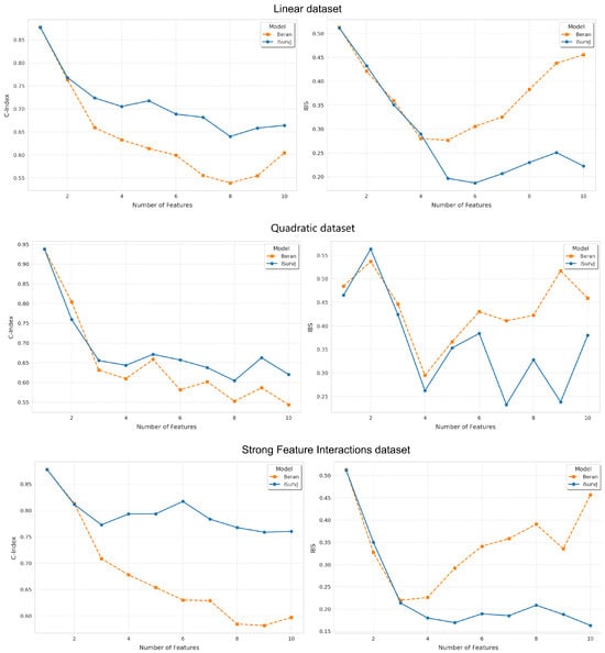
Figure 1.
Dependence of the C-index and IBS on the number of features for the Linear, Quadratic, Strong Feature Interactions datasets.

Figure 2.
Dependence of the C-index and IBS on the number of features for the Sparse Features, Nonlinear, and Noisy datasets.
6.3.2. Dependence on Parameter k
The next question was how parameter k in (29) impacted the model accuracy. We used the Friedman1, Friedman2, and Friedman3 synthetic datasets. The parameters of the model iSurvJ were the same as in the previous experiments. The number of features was five. The proportion of censored data in the dataset was . Values of the parameter k varied from 0 to 20 in increments of 1.
Results are shown in Figure 3. It can be seen from Figure 3 that the model’s accuracy significantly improves as the parameter k increases, but beyond a certain threshold, the improvement plateaus. At the same time, increasing k also raises the computational complexity. Therefore, beyond a certain value, further increasing k becomes pointless.
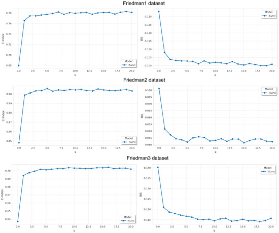
Figure 3.
Dependence of the C-index and IBS on parameter k for the Friedman1, Friedman2, and Friedman3 datasets.
6.3.3. Dependence on the Number of Censored Observations
Another study question was how the model accuracy depended on the number of censored instances. We used the Strong Feature Interactions and Sparse Features synthetic datasets with five features. The proportion of censored data in each dataset varied from 0 to in increments of . The parameters of iSurvJ were the same as in the previous experiments.
Figure 4 shows the dependence of the C-index and IBS on the proportion of censored data. The experimental results primarily illustrate how the accuracy of the proposed model decreased as the proportion of censored data increased.
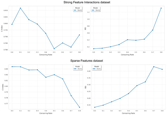
Figure 4.
Dependence of the C-index and IBS on the proportion of censored data for the Strong Feature Interactions and Sparse Features datasets.
The comparative experiments are illustrated in Figure 5, Figure 6 and Figure 7, which show the proposed model compared to the Beran estimator as the proportion of censored data increases. The average Kolmogorov–Smirnov (KS) distances between SFs obtained by these models for the same instances are also shown, depending on the proportion of censored data. The comparison results are provided for the Linear, Quadratic, Strong Feature Interactions, Friedman1, Friedman2, Friedman3, Sparse Features, Nonlinear, and Noisy datasets. The key feature of these comparative experiments was that instead of the iSurvJ model, we used the iSurvJ(G) model, where the neural network attention mechanism was replaced with a Gaussian kernel featuring a learnable parameter. It is interesting to point out from Figure 5, Figure 6 and Figure 7 that iSurvJ(G) outperformed the Beran estimator especially when the number of censored instances was large. This is clearly demonstrated by the KS distances, which show how the difference between SFs of two models increases with the proportion of censored data.
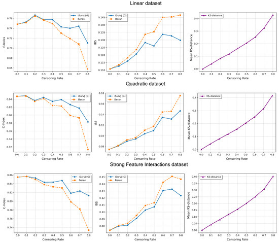
Figure 5.
Comparison of iSurvJ(G) and the Beran estimator for different values of the censored observation proportion for the Linear, Quadratic, and Strong Feature Interactions datasets.
Figure 6.
Comparison of iSurvJ(G) and the Beran estimator for different values of the censored observation proportion for the Friedman1, Friedman2, and Friedman3 datasets.
Figure 7.
Comparison of iSurvJ(G) and the Beran estimator for different values of the censored observation proportion for the Sparse Features, Nonlinear, and Noisy datasets.
6.3.4. Intervals for Survival Functions
The next experiments illustrated intervals of SFs depicted in Figure 8 and Figure 9. The plots are shown for one instance from a dataset (similar patterns can be observed for other instances and other datasets). One SF was produced as the prediction for this instance by the iSurvJ(G) model. Another SF was obtained as a prediction using the Beran estimator.
Figure 8.
Interval-valued SFs for the Friedman1 dataset for different values of the censoring rate.
Figure 9.
Interval-valued SFs for the Nonlinear dataset for different values of the censoring rate.
The bounds for the SF were obtained using (11), where probabilities , are interval-valued for censored observations. The attention weights were computed by using Gaussian kernels. As a result, we obtained the interval-valued probability distribution , , for the jth instance, which produced the interval-valued SFs, depicted in Figure 8 and Figure 9 for instances from the Friedman1 and Nonlinear datasets, respectively.
It is important to note that the Beran estimator predicted an SF which is totally inside the lower and upper SF bounds. This is a very interesting observation.
6.3.5. Unconditional Survival Functions
Let us study the relationship between the unconditional SFs produced by iSurvJ and the Kaplan–Meier estimator. The unconditional SF was calculated by averaging all conditional SFs obtained for all instances from a dataset. We considered the following real datasets: Veterans Lung Cancer, GBSG2, WHAS500, and Breast Cancer. Numerical features were standardized; categorical features were encoded. the parameters of iSurvJ were as follows: the number of epochs was 1000, the learning rate was , , the mask rate was 0, the regularization coefficient for weights was , the embedding dimension was 64, the batch_rate was , and the dropout rate was .
Figure 10 and Figure 11 illustrate the unconditional SFs obtained by iSurvJ and the Kaplan–Meier estimator. One can see from the plots that the SFs of both models are very close to each other.

Figure 10.
Unconditional SFs for the Veterans and GBSG2 datasets.
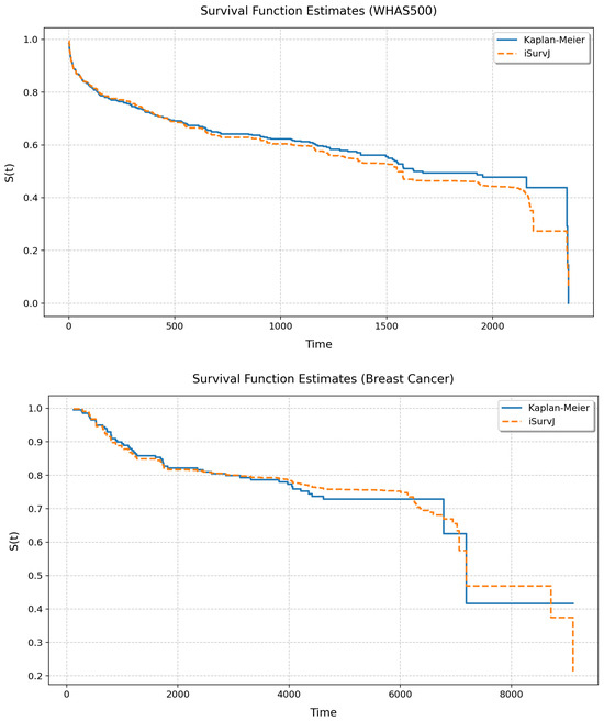
Figure 11.
Unconditional SFs for the WHAS500 and Breast Cancer datasets.
6.3.6. An Illustrative Comparative Example of iSurvJ(G) and Beran Estimator
To demonstrate the quality of the proposed approach, a synthetic dataset was generated in which the true relationship between a feature and the time to event was given by the following parabolic function:
where corresponds to the position of the minimum.
Features were generated to ensure a non-uniform observation density in different intervals: 200 points uniformly distributed in the interval , 10 points located in the interval , and 200 points uniformly distributed in the interval . Thus, the total number of observations was , with the central region corresponding to the smallest time-to-event values artificially thinned to reduce event density.
For the left and right parts of the sample, the censoring indicator was determined randomly according to the Bernoulli scheme with probability . For the central part of the parabola containing 10 observations, the censoring indicators were set manually, alternately taking values zero and one, which ensured diversity of observations in the region of the minimum. The iSurvJ(G) model was used in the experiment with 50 epochs, a learning rate of 7, , , a batch_rate of 1. In the Beran estimator, the same kernel as in iSurvJ(G) was used.
Results of the experiment are shown in Figure 12, which clearly demonstrates that the Beran estimator exhibits unstable behavior and fails to learn effectively from the given data, while the proposed model iSurvJ(G) with the same kernel successfully handles the complex data structure.
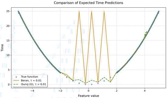
Figure 12.
Comparison of predicted expected times obtained by the Beran estimator and iSurvJ(G).
6.4. Some Conclusions from Numerical Experiments
The proposed models consistently outperformed the Beran estimator across synthetic datasets (Linear, Quadratic, Strong Feature Interactions, etc.), with the performance gap widening as the number of features increased (see Figure 1 and Figure 2). This suggests that iSurvJ is better suited for datasets with complex, high-dimensional feature structures. As the proportion of censored data increased, the Beran estimator exhibited instability, while iSurvJ(G) maintained robust performance (see Figure 5, Figure 6 and Figure 7). The Kolmogorov–Smirnov (KS) distances between SFs further confirmed that iSurvJ(G)’s predictions diverged significantly from the Beran estimator under heavy censoring, highlighting its adaptability.
The interval-valued SFs generated by the interval-valued representation of the instance probability distributions over the time intervals (see Figure 8 and Figure 9) encapsulated the Beran estimator’s predictions within the bounds, suggesting that the proposed model provides a more comprehensive representation of uncertainty, especially for censored observations.
The parameter k, controlling the neighborhood of intervals for uncensored data, initially improved accuracy but plateaued beyond a threshold (see Figure 3). This indicates a trade-off between the computational cost and marginal gains in predictive performance.
The unconditional SFs produced by iSurvJ closely matched those of the nonparametric Kaplan–Meier estimator (see Figure 10 and Figure 11), validating its consistency with classical methods while offering conditional predictions.
To compare the performance of iSurvJ(G) and the Beran estimator, we presented an illustrative example using a synthetic dataset generated with a parabolic time-to-event function (see Figure 12). The example demonstrated unstable behavior of the Beran estimator trained on specific complex data, whereas iSurvJ(G) with the same kernel successfully captured the underlying data structure.
In a nutshell, the experimental results demonstrated the superior performance of the proposed iSurvJ and iSurvJ(G) models compared to the traditional Beran estimator, particularly in high-dimensional and censored-data scenarios.
It should be noted that the models’ performance relies on hyperparameter tuning (e.g., embedding dimensions, regularization coefficients), though Optuna-based optimization mitigated this. While iSurvJ(G) uses a simpler Gaussian kernel, the neural network-based iSurvJ may face scalability issues with large datasets.
The main challenge with comparing our model to available transformer-based or deep learning survival models is that they require large volumes of data. For example, the authors of DeepHit [67] trained their model on the SEER dataset, which consists of 72,809 patients, or on a SYNTHETIC dataset of 30,000 patients. It is difficult to train deep learning survival models on small datasets due to the risk of overfitting. However, we compared our results with those of different models trained on the METABRIC dataset. The best corresponding C-index results, as presented in [16], were as follows: DeepSurv [68] 0.645; DeepHit 0.636; transformer-based deep survival model [16] 0.640. Models iSurvJ 0.647; iSurvJ(G) 0.6407. These results show that iSurvJ achieved the best performance, while the iSurvJ(G) variant remained competitive with the other models.
As a computational complexity example, we compared models iSurvJ and iSurvJ(G) trained on the synthetic Quadratic dataset. For a task with 500 instances and five features using 200 epochs, the learning time for iSurvJ(G) was 505 ms, compared to 808 ms for iSurvJ. The neural network implementing the function (see (13)) produced an embedding of size 64 for both models. The results showed a significant difference in learning time. However, their inference times were found to be approximately equal.
7. Conclusions
This work has introduced three novel survival models: iSurvM, iSurvQ, and iSurvJ, leveraging the imprecise probability theory and attention mechanisms to address censored-data challenges. One of the contributions is flexible modeling which means that the proposed framework avoids parametric assumptions and accommodates interval-valued probabilities for censored instances, enabling richer uncertainty quantification. We also have to point out that iSurvJ and its Gaussian-kernel variant iSurvJ(G) consistently outperformed the Beran estimator, particularly in high-dimensional settings and under heavy censoring.
The attention weights can be interpreted as a quantitative contribution measure within the example-based explanation framework [69]. In this approach, the most similar instances to a given sample are retrieved from the dataset to explain the model’s output—in this case, the survival function. This provides an advanced method for identifying influential instances, directly answering the question: “Which training instances were most responsible for this specific prediction?”
It should be noted that the proposed models deal with the standard survival analysis task. At the same time, it is interesting to extend it to competing risks and time-varying covariates. These are directions for further research. Moreover, we considered only small and middle-dimensional data. Another important direction for further research is to investigate scalability enhancements for ultra-high-dimensional data.
An extreme case of imprecision is when probabilities of time-to-event for the censored observations are in intervals from zero to one. There exist imprecise models and approaches which allow us to reduce the intervals employing additional assumptions, for example, applying definitions of reachable probability intervals [70] or survival models based on imprecise Dirichlet distribution [38].
Author Contributions
Conceptualization, L.U., A.K. and V.M.; methodology, L.U., V.M. and N.V.; software, A.K., V.E. and A.L.; validation, A.K., V.E., N.V., V.M. and A.L.; formal analysis, A.K. and L.U.; investigation, L.U., A.K., N.V. and V.M.; resources, L.U. and V.M.; data curation, V.M., A.L. and V.E.; writing—original draft preparation, L.U., N.V. and A.K.; writing—review and editing, L.U., N.V. and V.M.; visualization, V.E. and A.K.; supervision, L.U.; project administration, V.M.; funding acquisition, L.U. All authors have read and agreed to the published version of the manuscript.
Funding
This work was supported by the Russian Science Foundation under grant 25-11-00021.
Institutional Review Board Statement
Not applicable.
Informed Consent Statement
Not applicable.
Data Availability Statement
The data presented in this study are available in several public repositories. Data were derived from the resources available in the public domain and described in Section 6.2. [AIDS] [https://www.kaggle.com/datasets/tanshihjen/aids-clinical-trials] (accessed on 14 September 2025).
Acknowledgments
The authors would like to express their appreciation to the anonymous referees whose very valuable comments have improved the paper.
Conflicts of Interest
The authors declare no conflicts of interest.
Appendix A
Proof of Proposition 1.
First, decompose the norm:
The second term is as it is a classical Nadaraya–Watson’s error.
The first term can be bounded as follows:
It remains to derive the error bound on .
We find the vector as a minimizer of the loss function (26), which is a negative log-likelihood calculated for the kernel regression predictions. It can be seen that since estimates the vector as a Nadaraya–Watson regressor, then , the loss is Lipschitz continuous (given sufficient ), and the following holds
Then, taking into account that minimize the empirical loss function, minimizes the expected loss function, and the generalization bound assumption holds
therefore, for the expected loss functions, we obtain
By using the Pinsker’s inequality, we write
Combining the above, we obtain
Substituting this back into (A2) establishes the claimed rate for , since dominates . □
References
- Hosmer, D.; Lemeshow, S.; May, S. Applied Survival Analysis: Regression Modeling of Time to Event Data; John Wiley & Sons: Hoboken, NJ, USA, 2008. [Google Scholar]
- Jing, B.; Zhang, T.; Wang, Z.; Jin, Y.; Liu, K.; Qiu, W.; Ke, L.; Sun, Y.; He, C.; Hou, D.; et al. A deep survival analysis method based on ranking. Artif. Intell. Med. 2019, 98, 1–9. [Google Scholar] [CrossRef] [PubMed]
- Hao, L.; Kim, J.; Kwon, S.; Ha, I.D. Deep learning-based survival analysis for high-dimensional survival data. Mathematics 2021, 9, 1244. [Google Scholar] [CrossRef]
- Lee, E.; Wang, J. Statistical Methods for Survival Data Analysis; John Wiley & Sons: Hoboken, NJ, USA, 2003. [Google Scholar]
- Hothorn, T.; Bühlmann, P.; Dudoit, S.; Molinaro, A.; van der Laan, M. Survival ensembles. Biostatistics 2006, 7, 355–373. [Google Scholar] [CrossRef]
- Wrobel, L.; Gudys, A.; Sikora, M. Learning rule sets from survival data. BMC Bioinform. 2017, 18, 285–297. [Google Scholar] [CrossRef] [PubMed]
- Zhao, L.; Feng, D. DNNSurv: Deep Neural Networks for Survival Analysis Using Pseudo Values. arXiv 2019, arXiv:1908.02337v2. [Google Scholar]
- Zhao, Z.; Zobolas, J.; Zucknick, M.; Aittokallio, T. Tutorial on survival modeling with applications to omics data. Bioinformatics 2024, 40, btae132. [Google Scholar] [CrossRef]
- Marinos, G.; Kyriazis, D. A Survey of Survival Analysis Techniques. In Proceedings of the HEALTHINF, Online, 11–13 February 2021; pp. 716–723. [Google Scholar] [CrossRef]
- Wang, P.; Li, Y.; Reddy, C. Machine Learning for Survival Analysis: A Survey. ACM Comput. Surv. (CSUR) 2019, 51, 1–36. [Google Scholar] [CrossRef]
- Wiegrebe, S.; Kopper, P.; Sonabend, R.; Bischl, B.; Bender, A. Deep learning for survival analysis: A review. Artif. Intell. Rev. 2024, 57, 1–34. [Google Scholar] [CrossRef]
- Ishwaran, H.; Kogalur, U. Random Survival Forests for R. R News 2007, 7, 25–31. [Google Scholar]
- Belle, V.V.; Pelckmans, K.; Suykens, J.; Huffel, S.V. Survival SVM: A practical scalable algorithm. In Proceedings of the ESANN, Bruges, Belgium, 23–25 April 2008; pp. 89–94. [Google Scholar]
- Chen, G.H. An Introduction to Deep Survival Analysis Models for Predicting Time-to-Event Outcomes. Found. Trends Mach. Learn. 2024, 17, 921–1100. [Google Scholar] [CrossRef]
- Arroyo, A.; Cartea, A.; Moreno-Pino, F.; Zohren, S. Deep attentive survival analysis in limit order books: Estimating fill probabilities with convolutional-transformers. Quant. Financ. 2024, 24, 35–57. [Google Scholar] [CrossRef]
- Hu, S.; Fridgeirsson, E.; van Wingen, G.; Welling, M. Transformer-based deep survival analysis. In Proceedings of the Survival Prediction-Algorithms, Challenges and Applications, PMLR, Palo Alto, CA, USA, 22–24 March 2021; pp. 132–148. [Google Scholar]
- Li, C.; Zhu, X.; Yao, J.; Huang, J. Hierarchical Transformer for Survival Prediction Using Multimodality Whole Slide Images and Genomics. In Proceedings of the 26th International Conference on Pattern Recognition (ICPR), Montreal, QC, Canada, 21–25 August 2022; IEEE Computer Society: Los Alamitos, CA, USA, 2022; pp. 4256–4262. [Google Scholar] [CrossRef]
- Zhang, X.; Mehta, D.; Hu, Y.; Zhu, C.; Darby, D.; Yu, Z.; Merlo, D.; Gresle, M.; Van Der Walt, A.; Butzkueven, H.; et al. Adaptive transformer modelling of density function for nonparametric survival analysis. Mach. Learn. 2025, 114, 31. [Google Scholar] [CrossRef]
- Kaplan, E.; Meier, P. Nonparametric Estimation from Incomplete Observations. J. Am. Stat. Assoc. 1958, 53, 457–481. [Google Scholar] [CrossRef]
- Beran, R. Nonparametric regression with randomly censored survival data. In Technical Report; University of California: Berkeley, CA, USA, 1981. [Google Scholar]
- Chen, G.H. Survival kernets: Scalable and interpretable deep kernel survival analysis with an accuracy guarantee. J. Mach. Learn. Res. 2024, 25, 1–78. [Google Scholar]
- Evers, L.; Messow, C.M. Sparse kernel methods for high-dimensional survival data. Bioinformatics 2008, 24, 1632–1638. [Google Scholar] [CrossRef] [PubMed]
- Gefeller, O.; Michels, P. A review on smoothing methods for the estimation of the hazard rate based on kernel functions. In Proceedings of the Computational Statistics: Volume 1: Proceedings of the 10th Symposium on Computational Statistics, Neuchatel, Switzerland, August 1992; Springer: Berlin/Heidelberg, Germany, 1992; pp. 459–464. [Google Scholar] [CrossRef]
- Cawley, G.; Talbot, N.; Janacek, G.; Peck, M. Bayesian kernel learning methods for parametric accelerated life survival analysis. In Proceedings of the First International Conference on Deterministic and Statistical Methods in Machine Learning, Sheffield, UK, 7–10 September 2004; pp. 37–55. [Google Scholar] [CrossRef]
- Li, H.; Luan, Y. Kernel Cox regression models for linking gene expression profiles to censored survival data. In Proceedings of the Pacific Symposium Biocomputing 2003; World Scientific: Singapore, 2002; pp. 65–76. [Google Scholar] [CrossRef]
- Rong, Y.; Zhao, S.D.; Zheng, X.; Li, Y. Kernel Cox partially linear regression: Building predictive models for cancer patients’ survival. Stat. Med. 2024, 43, 1–15. [Google Scholar] [CrossRef] [PubMed]
- Yang, H.; Zhu, H.; Ahn, M.; Ibrahim, J.G. Weighted functional linear Cox regression model. Stat. Methods Med. Res. 2021, 30, 1917–1931. [Google Scholar] [CrossRef]
- Cox, D. Regression models and life-tables. J. R. Stat. Soc. Ser. (Methodol.) 1972, 34, 187–220. [Google Scholar] [CrossRef]
- Tutz, G.; Schmid, M. Modeling Discrete Time-to-Event Data; Springer: New York, NY, USA, 2016; Volume 3. [Google Scholar] [CrossRef]
- Suresh, K.; Severn, C.; Ghosh, D. Survival prediction models: An introduction to discrete-time modeling. BMC Med. Res. Methodol. 2022, 22, 207. [Google Scholar] [CrossRef]
- Kvamme, H.; Borgan, Ø. Continuous and discrete-time survival prediction with neural networks. Lifetime Data Anal. 2021, 27, 710–736. [Google Scholar] [CrossRef]
- Zhong, C.; Tibshirani, R. Survival analysis as a classification problem. arXiv 2019, arXiv:1909.11171v2. [Google Scholar] [CrossRef]
- Nadaraya, E. On estimating regression. Theory Probab. Its Appl. 1964, 9, 141–142. [Google Scholar] [CrossRef]
- Watson, G. Smooth regression analysis. Sankhya Indian J. Stat. Ser. 1964, 26, 359–372. [Google Scholar]
- Luong, T.; Pham, H.; Manning, C. Effective approaches to attention-based neural machine translation. In Proceedings of the 2015 Conference on Empirical Methods in Natural Language Processing; Association for Computational Linguistics: Lisbon, Portugal, 2015; pp. 1412–1421. [Google Scholar] [CrossRef]
- Vaswani, A.; Shazeer, N.; Parmar, N.; Uszkoreit, J.; Jones, L.; Gomez, A.; Kaiser, L.; Polosukhin, I. Attention is all you need. In Proceedings of the Advances in Neural Information Processing Systems, Long Beach, CA, USA, 4–9 December 2017; pp. 5998–6008. [Google Scholar]
- Kvamme, H.; Borgan, O.; Scheel, I. Time-to-Event Prediction with Neural Networks and Cox Regression. J. Mach. Learn. Res. 2019, 20, 1–30. [Google Scholar]
- Coolen, F. An imprecise Dirichlet model for Bayesian analysis of failure data including right-censored observations. Reliab. Eng. Syst. Saf. 1997, 56, 61–68. [Google Scholar] [CrossRef]
- Coolen, F.; Yan, K. Nonparametric predictive inference withright-censored data. J. Stat. Plan. Andin. 2004, 126, 25–54. [Google Scholar] [CrossRef]
- Mangili, F.; Benavoli, A.; de Campos, C.; Zaffalon, M. Reliable survival analysis based on the Dirichlet process. Biom. J. 2015, 57, 1002–1019. [Google Scholar] [CrossRef]
- Tang, Z.; Liu, L.; Chen, Z.; Ma, G.; Dong, J.; Sun, X.; Zhang, X.; Li, C.; Zheng, Q.; Yang, L.; et al. Explainable survival analysis with uncertainty using convolution-involved vision transformer. Comput. Med. Imaging Graph. 2023, 110, 102302. [Google Scholar] [CrossRef]
- Wang, Y.; Kong, X.; Bi, X.; Cui, L.; Yu, H.; Wu, H. ResDeepSurv: A Survival Model for Deep Neural Networks Based on Residual Blocks and Self-attention Mechanism. Interdiscip. Sci. Comput. Life Sci. 2024, 16, 405–417. [Google Scholar] [CrossRef]
- Salerno, S.; Li, Y. High-dimensional survival analysis: Methods and applications. Annu. Rev. Stat. Its Appl. 2023, 10, 25–49. [Google Scholar] [CrossRef]
- Bender, A.; Rügamer, D.; Scheipl, F.; Bischl, B. A general machine learning framework for survival analysis. In Proceedings of the Joint European Conference on Machine Learning and Knowledge Discovery in Databases, Ghent, Belgium, 14–18 September 2020; Springer: Berlin/Heidelberg, Germany, 2020; pp. 158–173. [Google Scholar] [CrossRef]
- Emmert-Streib, F.; Dehmer, M. Introduction to Survival Analysis in Practice. Mach. Learn. Knowl. Extr. 2019, 1, 1013–1038. [Google Scholar] [CrossRef]
- Chen, G.H. Deep kernel survival analysis and subject-specific survival time prediction intervals. In Proceedings of the Machine Learning for Healthcare Conference, PMLR, Durham, NC, USA, 7–8 August 2020; pp. 537–565. [Google Scholar]
- Yang, X.; Qiu, H. Deep Gated Neural Network With Self-Attention Mechanism for Survival Analysis. IEEE J. Biomed. Health Inform. 2024, 29, 2945–2956. [Google Scholar] [CrossRef] [PubMed]
- Wang, Z.; Sun, J. Survtrace: Transformers for survival analysis with competing events. In Proceedings of the 13th ACM International Conference on Bioinformatics, Computational Biology and Health Informatics, Chicago, IL, USA, 7–10 August 2022; pp. 1–9. [Google Scholar] [CrossRef]
- Jiang, S.; Suriawinata, A.A.; Hassanpour, S. MHAttnSurv: Multi-head attention for survival prediction using whole-slide pathology images. Comput. Biol. Med. 2023, 158, 106883. [Google Scholar] [CrossRef] [PubMed]
- Teng, J.; Yang, L.; Wang, S.; Yu, J. A Semi-Supervised Transformer Survival Prediction Model for Lung Cancer. Adv. Funct. Mater. 2025, 35, 2419005. [Google Scholar] [CrossRef]
- Wang, Z.; Gao, Q.; Yi, X.; Zhang, X.; Zhang, Y.; Zhang, D.; Liò, P.; Bain, C.; Bassed, R.; Li, S.; et al. Surformer: An interpretable pattern-perceptive survival transformer for cancer survival prediction from histopathology whole slide images. Comput. Methods Programs Biomed. 2023, 241, 107733. [Google Scholar] [CrossRef] [PubMed]
- Yao, Z.; Chen, T.; Meng, L.; Wong, K.C. A Multi-head Attention Transformer Framework for Oesophageal Cancer Survival Prediction. In Proceedings of the 2024 4th International Conference on Artificial Intelligence, Robotics, and Communication (ICAIRC), Xiamen, China, 27–29 December 2024; IEEE: Piscataway, NJ, USA, 2024; pp. 309–313. [Google Scholar] [CrossRef]
- Hill, B.M. De Finetti’s theorem, induction, and A (n) or Bayesian nonparametric predictive inference (with discussion). Bayesian Stat. 1988, 3, 211–241. [Google Scholar]
- Walley, P. Inferences from multinomial data: Learning about a bag of marbles. J. R. Stat. Soc. Ser. 1996, 58, 3–57. [Google Scholar] [CrossRef]
- Harrell, F.; Califf, R.; Pryor, D.; Lee, K.; Rosati, R. Evaluating the yield of medical tests. J. Am. Med. Assoc. 1982, 247, 2543–2546. [Google Scholar] [CrossRef]
- May, M.; Royston, P.; Egger, M.; Justice, A.; Sterne, J. Development and validation of a prognostic model for survival time data: Application to prognosis of HIV positive patients treated with antiretroviral therapy. Stat. Med. 2004, 23, 2375–2398. [Google Scholar] [CrossRef]
- Uno, H.; Cai, T.; Pencina, M.; D’Agostino, R.; Wei, L.J. On the C-statistics for evaluating overall adequacy of risk prediction procedures with censored survival data. Stat. Med. 2011, 30, 1105–1117. [Google Scholar] [CrossRef]
- Brier, G. Verification of forecasts expressed in terms of probability. Mon. Weather. Rev. 1950, 78, 1–3. [Google Scholar] [CrossRef]
- Graf, E.; Schmoor, C.; Sauerbrei, W.; Schumacher, M. Assessment and comparison of prognostic classification schemes for survival data. Stat. Med. 1999, 18, 2529–2545. [Google Scholar] [CrossRef]
- Bahdanau, D.; Cho, K.; Bengio, Y. Neural machine translation by jointly learning to align and translate. arXiv 2014, arXiv:1409.0473. [Google Scholar]
- Rubinstein, R.; Kroese, D. Simulation and the Monte Carlo Method, 2nd ed.; Wiley: Hoboken, NJ, USA, 2008; p. 345. [Google Scholar] [CrossRef]
- Smith, N.; Tromble, R. Sampling uniformly from the unit simplex. In Technical Report 29; Johns Hopkins University: Baltimore, MD, USA, 2004. [Google Scholar]
- Gyorfi, L.; Kohler, M.; Krzyzak, A.; Walk, H. A Distribution-Free Theory of Nonparametric Regression; Springer: Berlin/Heidelberg, Germany, 2002. [Google Scholar] [CrossRef]
- Lei, Y.; Dogan, U.; Zhou, D.X.; Kloft, M. Data-dependent generalization bounds for multi-class classification. IEEE Trans. Inf. Theory 2019, 65, 2995–3021. [Google Scholar] [CrossRef]
- Akiba, T.; Sano, S.; Yanase, T.; Ohta, T.; Koyama, M. Optuna: A next-generation hyperparameter optimization framework. In Proceedings of the 25th ACM SIGKDD International Conference on Knowledge Discovery & Data Mining, Anchorage, AK, USA, 4–8 August 2019; pp. 2623–2631. [Google Scholar] [CrossRef]
- Demsar, J. Statistical comparisons of classifiers over multiple data sets. J. Mach. Learn. Res. 2006, 7, 1–30. [Google Scholar]
- Lee, C.; Zame, W.; Yoon, J.; van der Schaar, M. Deephit: A deep learning approach to survival analysis with competing risks. In Proceedings of the 32nd Association for the Advancement of Artificial Intelligence (AAAI) Conference, New Orleans, LA, USA, 2–7 February 2018; pp. 1–8. [Google Scholar] [CrossRef]
- Katzman, J.; Shaham, U.; Cloninger, A.; Bates, J.; Jiang, T.; Kluger, Y. DeepSurv: Personalized treatment recommender system using a Cox proportional hazards deep neural network. BMC Med. Res. Methodol. 2018, 18, 1–12. [Google Scholar] [CrossRef]
- Poché, A.; Hervier, L.; Bakkay, M.C. Natural example-based explainability: A survey. In Proceedings of the World Conference on Explainable Artificial Intelligence, Lisbon, Portugal, 26–28 July 2023; Springer: Berlin/Heidelberg, Germany, 2023; pp. 24–47. [Google Scholar] [CrossRef]
- Destercke, S.; Antoine, V. Combining Imprecise Probability Masses with Maximal Coherent Subsets: Application to Ensemble Classification. In Advances in Intelligent Systems and Computing, Proceedings of the Synergies of Soft Computing and Statistics for Intelligent Data Analysis; Springer: Berlin/Heidelberg, Germany, 2013; Volume 190, pp. 27–35. [Google Scholar] [CrossRef]


Disclaimer/Publisher’s Note: The statements, opinions and data contained in all publications are solely those of the individual author(s) and contributor(s) and not of MDPI and/or the editor(s). MDPI and/or the editor(s) disclaim responsibility for any injury to people or property resulting from any ideas, methods, instructions or products referred to in the content. |
© 2025 by the authors. Licensee MDPI, Basel, Switzerland. This article is an open access article distributed under the terms and conditions of the Creative Commons Attribution (CC BY) license (https://creativecommons.org/licenses/by/4.0/).