Abstract
With the advancement of autonomous driving technology, vehicle lane-change decision (LCD) has become a critical issue for improving driving safety and efficiency. Traditional deep reinforcement learning (DRL) methods face challenges such as slow convergence, unstable decisions, and low accuracy when dealing with complex traffic environments. To address these issues, this paper proposes a novel integrated deep reinforcement learning model called “SGD-TripleQNet” for autonomous vehicle lane-change decision-making. This method integrates three types of deep Q-learning networks (DQN, DDQN, and Dueling DDQN) and uses the Stochastic Gradient Descent (SGD) optimization algorithm to dynamically adjust the network weights. This dynamic weight adjustment process fine-tunes the weights based on gradient information to minimize the target loss function. The approach effectively addresses key challenges in autonomous driving lane-change decisions, including slow convergence, low accuracy, and unstable decision-making. The experiment shows that the proposed method, SGD-TripleQNet, has significant advantages over single models: In terms of convergence speed, it is approximately 25% faster than DQN, DDQN, and Dueling DDQN, achieving stability within 150 epochs; in terms of decision stability, the Q-value fluctuations are reduced by about 40% in the later stages of training; in terms of final performance, the average reward exceeds that of DQN (by 6.85%), DDQN (by 6.86%), and Dueling DDQN (by 6.57%), confirming the effectiveness of the proposed method. It also provides a theoretical foundation and practical guidance for the design and optimization of future autonomous driving systems.
Keywords:
autonomous driving; deep reinforcement learning; lane-change decision; stochastic gradient descent (SGD) optimization algorithm MSC:
90-10
1. Introduction
Autonomous driving systems, as cutting-edge technologies in the field of transportation, are centered around improving vehicle safety and decision-making efficiency [1,2]. The decision-making system, acting as the bridge between perception and control, not only needs to accurately understand complex road traffic environments but also must plan the optimal driving strategies for the vehicle [3]. Through artificial intelligence technologies such as deep reinforcement learning, the adaptability of the decision-making system in dynamic traffic scenarios can be significantly enhanced, reducing the risk of traffic accidents, optimizing traffic flow, and alleviating congestion issues [4]. Additionally, the research findings can be directly applied to improve existing driver assistance systems and promote the industrialization of autonomous driving technologies, bringing significant social benefits and economic value. With the rapid development of autonomous driving technology, lane-change decision-making has become an increasingly critical component in ensuring both safety and efficiency on the road [5,6]. Existing research indicates that behavioral decision-making models for autonomous vehicles can be divided into two main categories based on their underlying principles: rule-based methods and deep learning-based driving behavior decision models [7,8,9,10].
Rule-based driving behavior decision models guide vehicle behavior through human-designed rules or strategies. Before the advent of artificial intelligence, the implementation of lane-change decision (LCD) tasks was primarily solved using feedback control techniques [11]. These techniques typically used information collected from sensor measurements as input, employing classical control algorithms such as fuzzy logic models and LQR to stabilize vehicle behavior in simple lane-change tasks. With deeper research into the LCD problem, a new lane-change model was proposed that considers uncertainties or fuzzy factors and their relationships [12], which included simulations of mixed traffic flows at different penetration rates and demonstrated the impact of autonomous vehicle penetration and certain fuzziness on lane-change behavior. In the LQR approach, an improved LQR lateral motion control method for vehicle lane-changing with feedforward control was introduced, which enhanced control accuracy and adaptability [13]. However, these classical control methods generally require accurate mathematical models of the system, are better suited for simpler traffic scenarios, and often require the manual adjustment of tools and parameters. In dynamic or extreme environments, these methods may exhibit unstable behavior and cannot fully handle all unseen scenarios, thus posing safety risks [14,15].
With advances in technology and the continuous development of deep reinforcement learning (DRL), deep learning-based driving behavior decision models have become mainstream in research. These models generate decisions by learning from historical data or interacting with the environment, training deep neural networks [16]. In 2013, the DeepMind team introduced DRL through the Atari game platform, combining deep learning and reinforcement learning to train agents that automatically learn from environmental feedback (rewards), which sparked widespread interest in academia [17]. Researchers began using onboard sensors and communication network systems to gather scene information, focusing primarily on strategies to improve safety, comfort, and energy optimization for autonomous driving in complex environments. However, the research found that its generalization ability was poor, and it was difficult to implement in real-world environments. However, deep reinforcement learning-based lane-change decision frameworks were proposed to find the optimal decision-making strategy that minimizes the risks of autonomous driving [18,19]. However, compared to earlier methods, the end-to-end learning approach can more effectively handle complex and dynamic task environments [20]. Researchers then began studying integrated deep reinforcement learning models, combining Deep Deterministic Policy Gradient (DDPG) reinforcement learning with Long Short-Term Memory (LSTM) trajectory prediction models [21], significantly improving lane-change safety and efficiency. An improved Grey Wolf Optimization Deep Belief Network (DBN) model was introduced, effectively predicting the longitudinal and lateral positions of vehicles and enabling efficient lane-change prediction [22], but its stability was poor and lacked application in real-world traffic environments [23]. Subsequently, an integrated deep reinforcement learning-based driving behavior decision model for autonomous vehicles was proposed [24]. However, this model only used a simple voting mechanism to assign weights to a single model based on the current environmental state, and the data used were not from real-world environments, making it less capable of handling complex and dynamic traffic scenarios [25].
This paper proposes an ensemble deep reinforcement learning model, called SGD-TripleQNet. The model integrates three deep Q-learning networks and dynamically adjusts their individual weights through the Stochastic Gradient Descent (SGD) optimization algorithm to optimize the decision-making process. The weights are updated dynamically based on the loss functions of each model, enabling effective collaboration and performance enhancement between the models.
2. Materials
In this section, we introduce the advantages of the NGSIM dataset for vehicle LCD and describe the steps of data preprocessing, data filtering, and smoothing. These processes aim to enhance the model’s training performance and generalization ability, enabling a more accurate simulation of lane-change behavior in real-world traffic scenarios.
2.1. Environment Description
In LCD tasks, data quality plays a crucial role in ensuring the accuracy and reliability of decisions. A comprehensive dataset should encompass a wide range of real-world driving scenarios, including vehicle trajectories for straight driving, left turns, right turns, acceleration, and deceleration. Therefore, this study selects the NGSIM (Next Generation Simulation) dataset, a high-quality traffic data collection and simulation project initiated by the U.S. Department of Transportation, and specifically utilizes highway data without intersections to validate the vehicle lane-change model [26]. The NGSIM dataset provides detailed motion information for each vehicle on monitored road segments, recorded at 0.1-s intervals (such as speed, acceleration, and position). The dataset includes highway data collected at various locations and times, including segments of California’s US-101 and I-80, as well as urban street data from Peachtree Street in Atlanta and Lankershim Boulevard in Los Angeles. The US-101 and I-80 datasets are important sources of data for analyzing vehicle driving behavior. The data from the US-101 highway in California cover three time periods (each 15 s) between 7:50 and 8:35 a.m., reflecting different traffic flow and speed conditions. The data from the I-80 highway in California span three time periods (each 15 s) between 4:00 and 5:30 p.m., focusing on complex traffic scenarios such as highway merging and lane changing [27].
Both datasets are collected from multi-lane, bidirectional highways and provide detailed information on vehicle position, speed, acceleration, and headway distance. They include three different traffic flow conditions: sparse, medium-density, and dense. The I-80 dataset offers greater diversity in terms of traffic density and the number of lanes, and it features numerous merging sections. In contrast, the US-101 highway dataset is from a straight road environment with simpler scenarios, lacking complex highway merges or diverging lanes. This makes the US-101 dataset more suitable for early-stage research, as it allows the focus to be on lane-change behavior itself without the interference of complex traffic patterns. Therefore, this paper selects the US-101 as the lane-change environment for the study [28,29].
2.2. Data Filtering
The NGSIM (Next Generation Simulation) US-101 dataset includes data from three time periods: 7:50 a.m.–8:05 a.m., 8:05 a.m.–8:20 a.m., and 8:20 a.m.–8:35 a.m. These periods cover different traffic flow densities and dynamic variations during the morning rush hour. The data record traffic scenes ranging from sparse to medium-density to dense flow conditions. This paper analyzes vehicle behavior during these different time periods, as shown in the Figure 1.
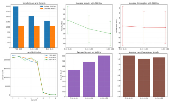
Figure 1.
Traffic flow density and behavior analysis charts for the time periods 7:50 a.m.–8:05 a.m., 8:05 a.m.–8:20 a.m., and 8:20 a.m.–8:35 a.m.
As shown in the figure above, the data from 8:05 a.m.–8:20 a.m. demonstrate optimal conditions in terms of traffic flow, stability, and lane-change behavior.
The lane utilization curve for the 8:05 a.m.–8:20 a.m. period is similar to other time intervals but exhibits a more balanced distribution of data, which is beneficial for analyzing vehicle behavior across different lanes. The number of unique vehicles and total records during this period are at moderate levels, and the moderate traffic flow is conducive to studying lane-change behavior. It helps to avoid the issue of sparse or overly congested data, which could make lane-change behavior less evident.
Furthermore, the standard deviations of average speed (Velocity) and average acceleration (Acceleration) are relatively small, indicating that vehicle behavior during this period is more consistent with less fluctuation in the data. This makes it an ideal time segment for the research and modeling of vehicle lane-change decision-making.
2.3. Data Preprocessing
We performed outlier handling and smoothing on the NGSIM dataset. The specific preprocessing steps include handling missing values, outliers, and data transformation, followed by smoothing using the Savitzky–Golay filter [30,31].
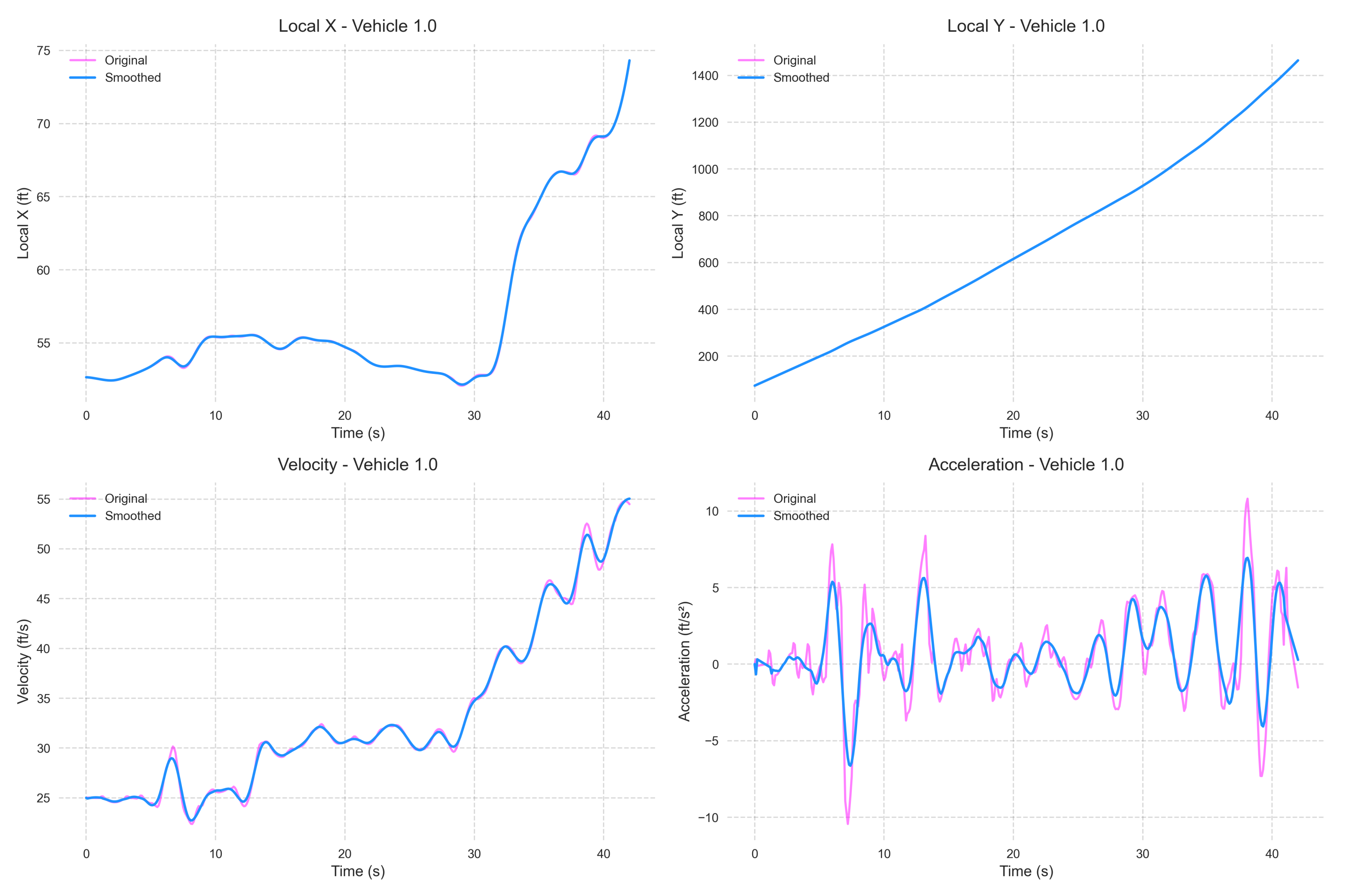
In real-world traffic data, raw position data often exhibit high volatility due to measurement errors and sensor noise. The Savitzky–Golay filter effectively preserves the trend of the signal while reducing the impact of noise on the results. To minimize the effect of noise and extract meaningful vehicle motion information from the traffic data, we applied the Savitzky–Golay filter for smoothing [32,33]. The following Figure 2 illustrates the smoothed curve when the filter window size is 25.

Figure 2.
A comparison chart of the smoothed vehicle speed, X and Y positions, and acceleration with the original data.
3. Background
In this section, we describe three individual deep reinforcement learning (DRL) models: DQN, DDQN, and Dueling DDQN, and provide a detailed introduction to their algorithmic principles and model structures.
3.1. DQN Model
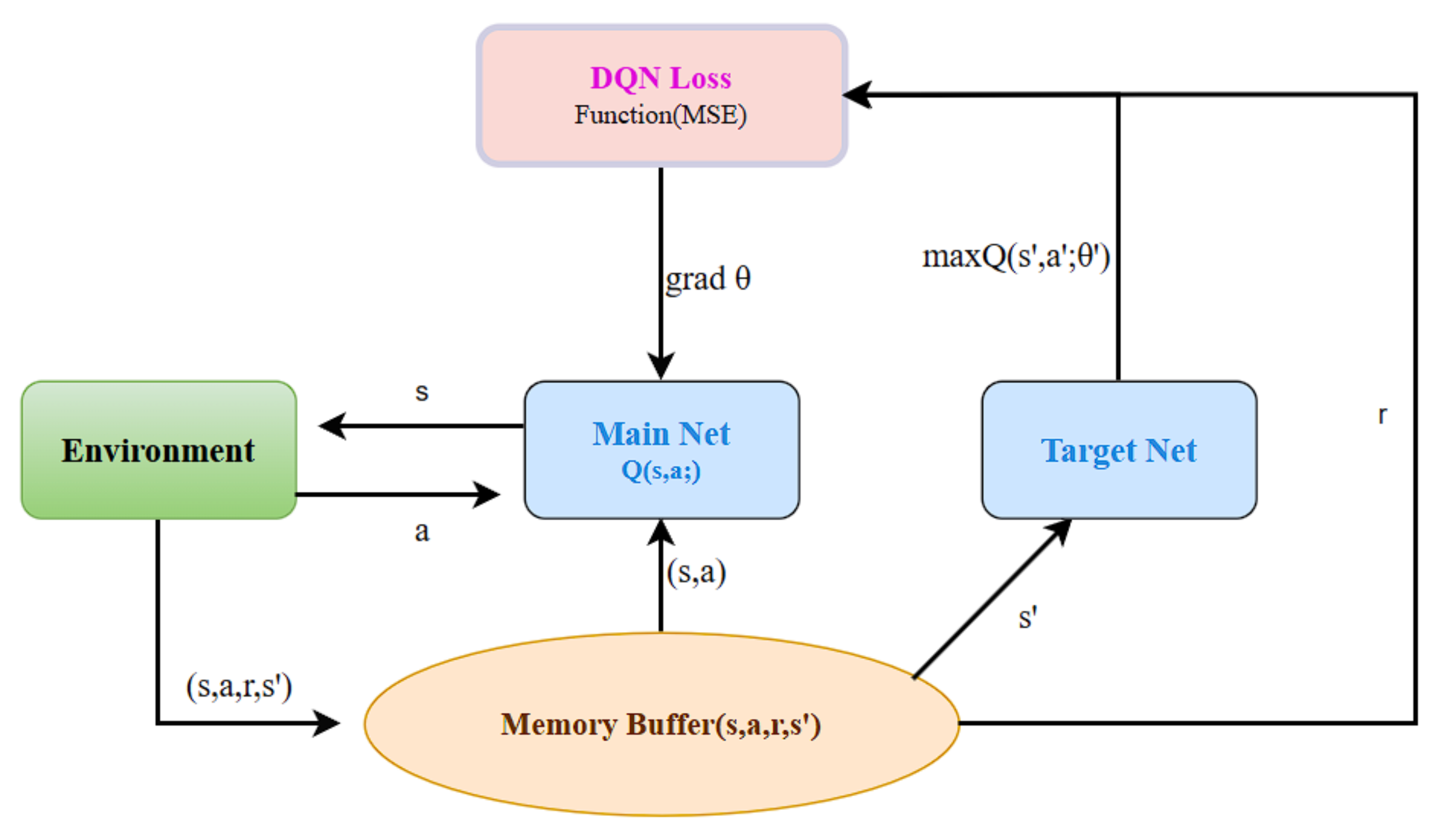
The Q-learning algorithm is the predecessor of the DQN (Deep Q-Network) algorithm. Q-learning was proposed by Watkins in 1989, while DQN is an algorithm that combines deep learning with reinforcement learning, introduced by the Google DeepMind team in 2015 [34]. DQN is a reinforcement learning algorithm based on Q-learning, enhanced by the incorporation of a deep convolutional neural network to approximate the value function, a simulation replay mechanism, and an independent target network. DQN is primarily designed to address issues in high-dimensional state spaces [35,36]. Reinforcement learning algorithms typically use Markov Decision Processes (MDP) to model reinforcement learning tasks. The specific implementation process is shown in Figure 3.

Figure 3.
DQN architecture diagram.
Where is the learning rate, is the discount factor, is the immediate reward obtained by the agent, and and represent the new state and the action taken in that state, respectively. In the lane-change decision-making task, DQN can estimate the future rewards for each lane-change option (such as left lane, middle lane, or right lane) by considering both the historical and current states, thereby guiding the decision-making process. In the model training process, the DQN model updates the parameters using gradient descent to optimize the loss function, which represents the difference between the target value network and the current value network outputs. The loss function is typically expressed by Equation (1):
where
is the loss function, representing the mean squared error between the target value network output and the current value network output. is the target value, given by , where represents the immediate reward from the environment at time t, is the discount factor, is the next state of the environment at time , represents the possible actions that can be taken in the next state , is the Q-value for the next state–action pair under the target value network parameters , and refers to the parameters of the target value network.
3.2. DDQN Model
DDQN (Double Deep Q-Network) is an improved version of DQN designed to address the overestimation problem inherent in DQN. The overestimation issue can lead to biased learning, which negatively impacts the performance of the policy. DDQN resolves this by splitting the maximization process in the target network into two parts: action selection using the current Q-network and action evaluation using the target Q-network. This approach effectively reduces the overestimation bias in DQN, thereby enhancing the model’s stability [36].
Although the two networks have different structures in the reinforcement learning task, they share the same input and output data types, making it possible to integrate them into a unified model. The target value calculation formula is shown in Equation (2).
where is the action chosen by the current online network (Online Network) for the next state , is the Q-value output by the target network (Target Network) for the next state and the selected action , is the discount factor, typically in the range of [0, 1], and is the immediate reward received at time step t.
This target value formulation reduces overestimation bias by using the online network to select the action and the target network to evaluate it.
3.3. Dueling DDQN Model
Dueling DDQN (Dueling Double Deep Q-Network) is a further improvement upon DDQN, combining the Dueling Network Architecture with the action selection and evaluation separation mechanism of DDQN. This mechanism enables more efficient learning in certain states, as it avoids the excessive optimization of irrelevant actions and addresses the learning efficiency issues faced by traditional Q-learning methods in some states [37]. This improves both the performance and stability of the model [38].
The core idea of Dueling Network Architecture is to decompose the Q-value into two components; this is shown in Equation (3).
The final state–action in Dueling DDQN can be expressed as shown in Equation (4):
where represents the state value, represents the advantage function, represents the hidden layer network parameters, represents the number of actions, represents the state value network parameters, and represents the action advantage network parameters.
4. Methods
In this section, we first define the state space using six features: vehicle speed, X/Y coordinates, current lane, and the distances to the front and rear vehicles. Next, we define the action space, which includes five actions: left lane change, right lane change, keep lane, accelerate, and decelerate. We then consider various reward and penalty factors for LCD and design a reward function that incorporates driving safety, traffic efficiency, driving comfort, lane-change behavior, and lane-keeping performance to ensure a comprehensive evaluation of the vehicle’s behavior under different traffic conditions. Finally, we provide a detailed introduction to the proposed SGD-TripleQNet model and its principles.
4.1. Set State Space
State Space is a core concept in reinforcement learning, used to describe the environmental state of an intelligent agent at a specific time [32]. The state space S represents the state information perceived by an autonomous driving vehicle while driving on the road, including the position (X, Y), velocity v, and acceleration a of both the ego vehicle and surrounding vehicles. Each state represents the current status of the vehicle, which serves as an input for the reinforcement learning model. The model selects actions based on the current state (State) and learns through a reward (Reward) function.
The state space consists of six key features, defined as a six-dimensional vector. Its function is represented by Equation (5):
where Presence indicates whether a vehicle exists; x represents the lateral position of the vehicle, indicating its position relative to the road laterally; and y represents the longitudinal position of the vehicle, indicating its position relative to the road longitudinally. v represents the real-time velocity of the vehicle in feet/second, reflecting the current dynamic state of the vehicle. P represents the state information of surrounding vehicles. The design of these state features can comprehensively describe the actual position and dynamic behavior of vehicles in the traffic environment.
4.2. Set Action Space
The action space is designed with five choices. In the autonomous vehicle behavior decision MDP model, the action space A (6) includes five driving behaviors to adapt to different driving scenarios: changing lanes to the left (), changing lanes to the right (), maintaining the current lane (), accelerating in the same lane (), and decelerating in the same lane ():
This design ensures that the agent can consider actual traffic rules when making decisions and avoid selecting invalid lane-changing actions.
4.3. Design Reward Function
4.3.1. Basic Safety Reward
This reward is primarily based on evaluating inter-vehicle distance. A positive reinforcement is given when the headway exceeds the safety threshold, with the reward proportional to the margin above the safe distance; a negative punishment is given when the distance falls below the safety threshold, with the penalty proportional to the safety deficit. This design aims to encourage vehicles to maintain safe distances and avoid rear-end collision risks [34,35]. Its reward function is represented by Equation (7).
where, Space_Hdwy (SH) represents the current headway distance, and SAFE_DISTANCE (SD) is the preset safety distance.
4.3.2. Traffic Efficiency Reward
This reward incorporates two factors: speed deviation, which is the absolute difference between current and target speeds, and time step penalty. By applying a negative reward to speed deviation, it guides vehicles to maintain speeds near the desired velocity while considering time costs to promote efficient traffic flow. Its reward function is represented by Equation (8)
where is the vehicle velocity, is the target velocity, and is the time step penalty.
4.3.3. Comfort Reward
The driving comfort is measured by evaluating vehicle acceleration and jerk (rate of change in acceleration), suppressing dramatic speed changes to enhance driving comfort. This paper designs the reward function using an inverse form, so that the smaller acceleration and jerk values result in larger rewards. Its reward function is represented by Equations (9) and (10).
where is the acceleration at time t, is the acceleration at the next time step, is the time step interval, jerk represents the rate of acceleration change, and is the comfort balance coefficient.
4.3.4. Lane-Change Behavior Reward
This component introduces a lane-change cooling mechanism. The agent receives a penalty for lane changes during the cooling period (T) to suppress frequent lane changes, provides a larger positive reward for lane changes outside the cooling period to support necessary lane-changing behavior, and gives a moderate positive reward for maintaining the current lane to encourage stable driving. If the agent chooses to change lanes or maintain the current lane, each action receives a reward of 5. The formula for its reward function is (11)
where represents the time elapsed since the last lane change and T is the cooling period threshold. A penalty is applied for lane changes during the cooling period (), a larger positive reward is given for lane changes after the cooling period (), and a moderate positive reward is given for maintaining the current lane (stay).
4.3.5. Violation Penalty
When the vehicle drives outside the normal lane boundaries, a significant negative penalty is applied to ensure that the vehicle always drives within the designated lanes. Its reward function is represented by Equation (12):
4.3.6. Final Total Reward
The final comprehensive reward can be expressed as the sum of the above five sub-rewards. This design enables the reward function to comprehensively evaluate vehicle lane-changing decision behavior. It balances traffic efficiency and driving comfort, effectively regulates vehicle lane-changing behavior, and weights each reward component to achieve optimal results, all while ensuring driving safety. The finall rewards function is represented by Equation (13).
where is the weighting coefficients for each sub-reward component .
4.4. SGD-TripleQNet Model
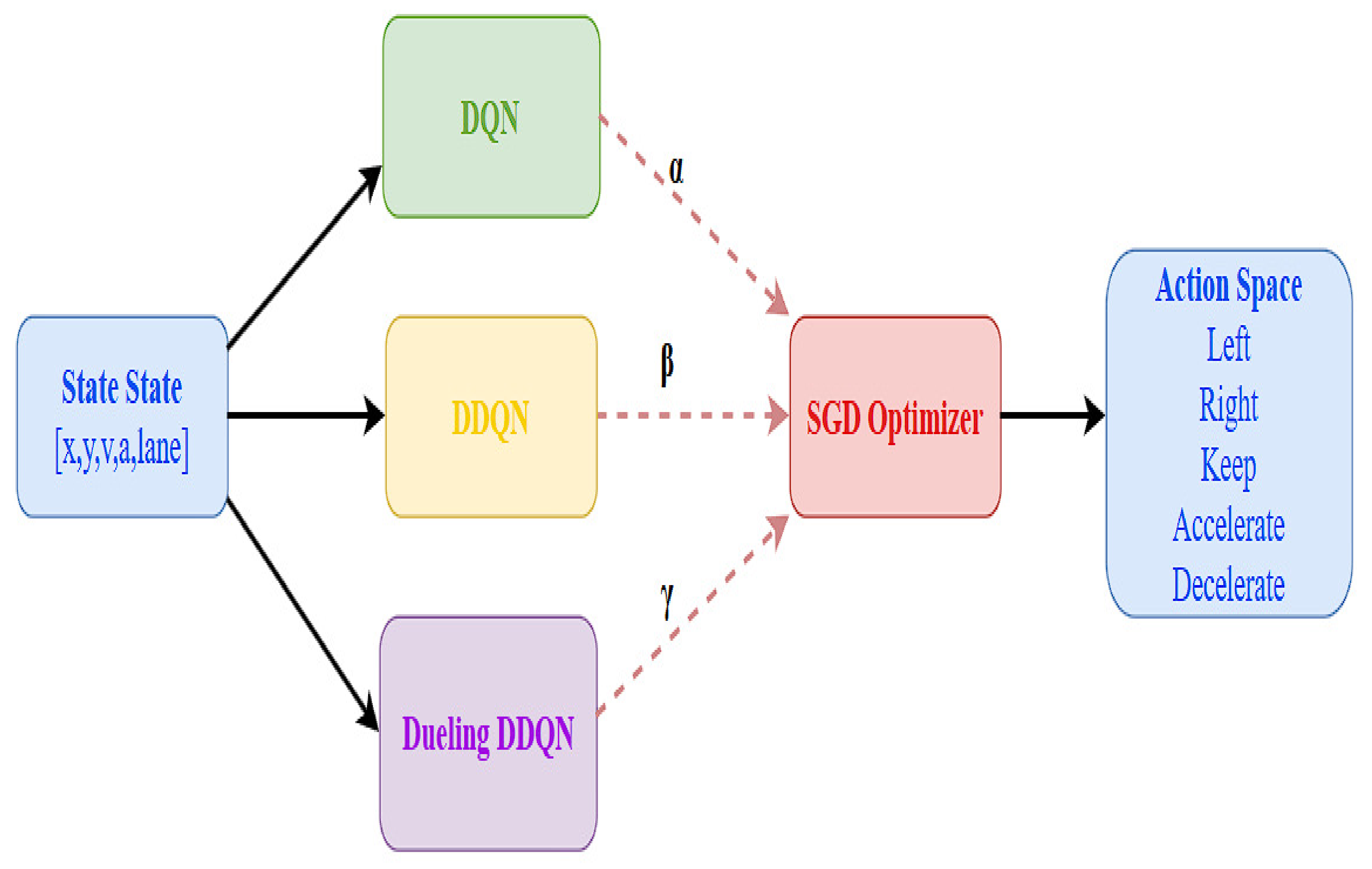
The core objective of this paper is to integrate three network models—DQN, DDQN, and Dueling DDQN—to collaboratively optimize lane-changing decisions through their respective advantages. At the start of model training, the initial weights , , and are assigned to each model. Initially, , which is used to distribute weights among different models, and an SGD optimizer is used to update these weights with a certain step size. Then, the Q-values for each model are calculated independently, denoted as , , and . The Q-value output of TripleQNet can be expressed in Equation (14).
where s represents the current state, and a represents the current chosen action (such as “lane left”, ”lane left”, “keep lane”, etc.). This method leverages the strengths of different models to achieve a more stable and robust policy.
After each training round, the gradient of the loss function is calculated, and the weights of each model are dynamically updated with a learning rate to minimize the total model loss. To prevent any model’s weight from becoming too large, an L2 regularization term is added to TripleQNet’s loss function (15) and (16).
The weights, shown in Equation (17), are updated according to the loss gradient during each epoch:
The updated weights are used for Q-value calculation in the next round, allowing the model to gradually optimize its performance. The architecture diagram of SGD-TripleQNet is shown in the Figure 4.

Figure 4.
Architecture diagram of SGD-TripleQNet.
4.5. DQN, DDQN, Dueling DDQN and SGD-TripleQNet Pseudocode
SGD-TripleQNet integrates the training processes of DQN, DDQN, and Dueling DDQN into a unified framework, leveraging the SGD algorithm to optimize the weights, thereby minimizing the total loss. Additionally, an L2 regularization method is incorporated to prevent any single model’s weight from becoming excessively large. The pseudocode for the SGD-TripleQNet algorithm, the individual DQN, DDQN, and Dueling DDQN is shown in Algorithm 1 below.
| Algorithm 1 DQN, DDQN, Dueling DDQN, and SGD-TripleQNet Training |
| 1: Initialize: state s, Input:, learning rate , L2 coefficient , initialized Q-learning networks: DQN, DDQN, Dueling DDQN, training dataset D, target network update frequency: T, batchsize. 2: Neural networks: DQN, DDQN, Dueling DDQN 3: Optimizers: Adam for each model 5: Action space: 6: State space: 7: Replay buffer: 8: For each episode = 1 to max_episodes: 9: Initialize state at time step 10: For each step to : 11: Choose action based on policy (e.g., epsilon-greedy) 12: Execute action , observe next state , and reward 13: Store transition in 14: If episode > warmup_steps: 15: Compute target : 16: For DQN: 17: For DDQN: 18: For Dueling DDQN: Similar to DDQN 19: Compute loss: 20: Perform gradient descent to minimize 21: Update target network every T steps 22: End if 23: End for 24: Update learning rates using SGD for SGD-TripleQNet: 25: Adjust weights for each model based on performance 26: Update weights using SGD: 28: 29: 30: End for 31: End |
5. Results
This section verifies the performance of the three individual models, DQN, DDQN, and Dueling DDQN, on lane-change decision (LCD) through training. It also implements an integrated model with optimized weight distribution using the SGD optimization algorithm, and discusses the training results, considering factors such as driving safety, lane change necessity, and comfort.
In the training process, we conducted model training over 1000 epochs and evaluated the model performance using various metrics including the loss function, Q-values, and rewards. We designed and conducted comparative experiments across four algorithms: traditional DQN, DDQN, Dueling DDQN, and the proposed SGD-TripleQNet. The stability of the SGD-TripleQNet model was evaluated, and the average rewards obtained by the agent under different policies were compared. In order to evaluate and compare the learning capabilities and stability characteristics of these algorithms, we conducted comprehensive training of three models: DQN, DDQN, and Dueling DDQN. Throughout the training process, we monitored and recorded both the evolution of loss values and weight convergence patterns, which are summarized in the subsequent table. The models were trained for 1000 epochs, and their final loss values and weight distributions are presented in Figure 5.
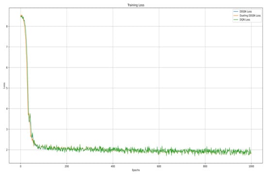
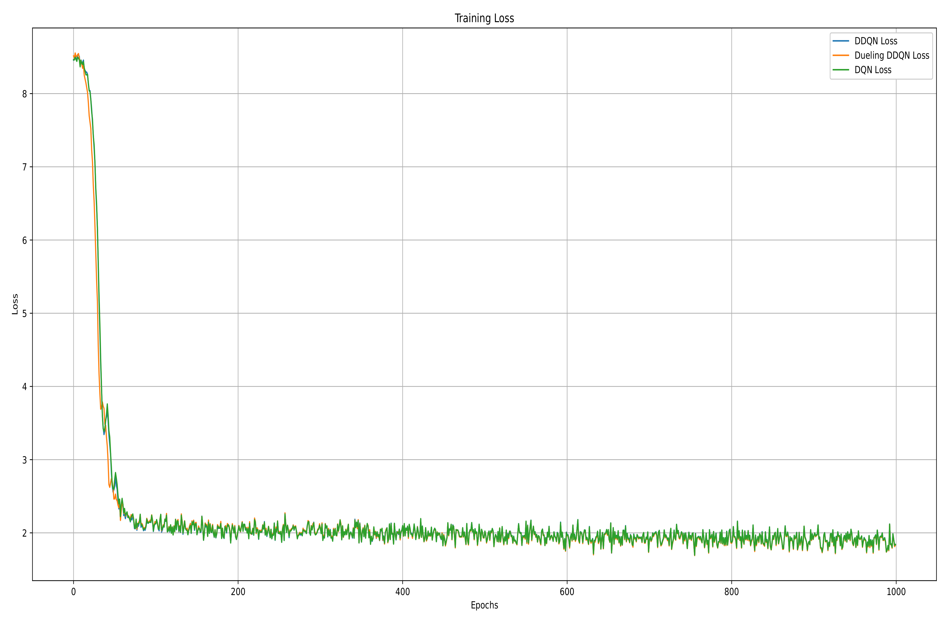
Figure 5.
DQN, DDQN, and Dueling DDQN training loss curves.
The training loss curves illustrate the convergence characteristics of three deep reinforcement learning models: DQN, DDQN, and Dueling DDQN. Initially, all three models start with a loss value of approximately 8.5. However, during the first 50 epochs, the loss rapidly decreases, indicating efficient initial learning and parameter optimization. Around the 100th epoch, the loss curve shows a clear inflection point, after which the rate of change gradually slows down. From epoch 200 onward, the loss stabilizes at around 2.0, with minimal fluctuations, indicating that the models have reached a stable convergence state. During the later stages of training (epochs 400 to 1000), the curves remain stable, validating the effectiveness of the chosen hyperparameters, gradient descent optimization method, and training strategy. All three models successfully converge and find their optimal parameters.
Finally, after 1000 epochs, the final loss values and the weights of the three models are shown in the Table 1 below.

Table 1.
Final loss values of DQN, DDQN, and Dueling DDQN after 1000 epochs.
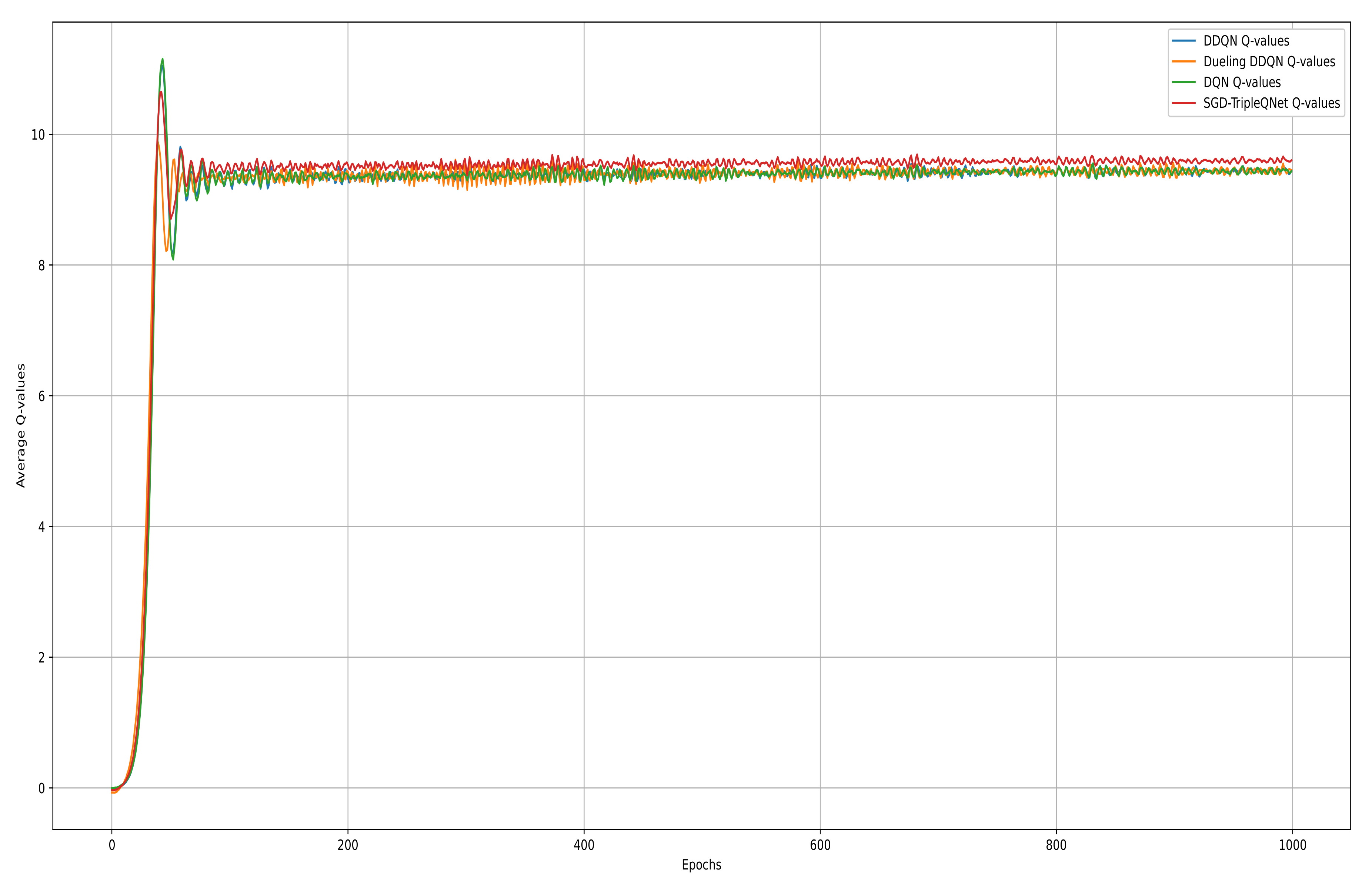
We plot the average Q-value curve and the average action–reward curve for four models during the training process in Figure 6 and Figure 7. The average Q-value curve represents the model’s estimate of the expected cumulative future reward, while the average action–reward curve reflects the agent’s average reward per action throughout the task. From the average Q-value curve, we can observe that in the early stages of training (0–50 epochs), all models exhibit a consistent rapid learning pattern, with Q-values quickly rising from 0 to a peak of 11. In the optimization phase (50–200 epochs), the SGD-TripleQNet model shows smaller oscillations (±0.3), while the single models exhibit relatively larger fluctuations (±0.5).

Figure 6.
Average Q-value curves of DQN, DDQN, Dueling DDQN, and SGD-TripleQNet.

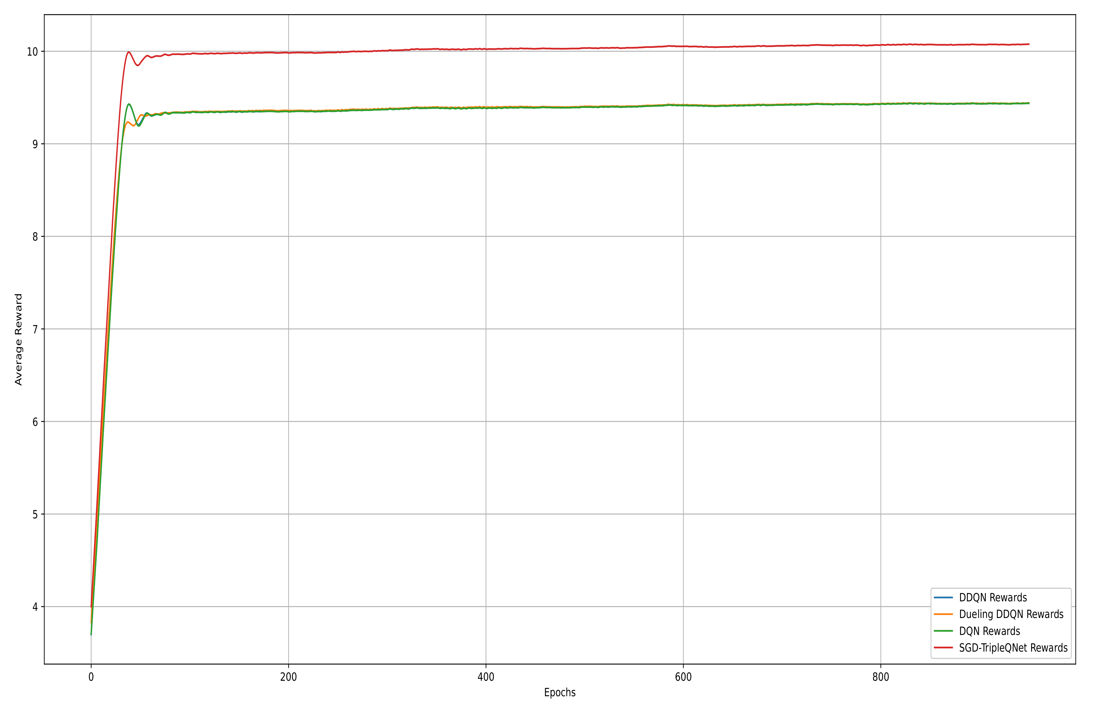
Figure 7.
Average reward curves of DQN, DDQN, Dueling DDQN, and SGD-TripleQNet.
Between 200 and 1000 epochs, the Q-value for SGD-TripleQNet stabilizes at around 9.7 ± 0.1, which is approximately 2.1% higher than the single models, which stabilize at 9.5 ± 0.15. All four models eventually converge and stabilize, reflecting an accurate estimation of state–action values and validating the model’s strong generalization ability and decision-making performance. However, the performance of Dueling DDQN is similar to that of DQN, indicating that the separation of state value and advantage function does not provide a significant advantage in this LCD task.
The average reward curve clearly demonstrates the model’s performance in real-world decision-making. Starting from an initial random policy level (around 3.7), the model rapidly improves within the first 50 epochs. SGD-TripleQNet reaches an average reward of 9.8 at epoch 75, while the three single models stabilize around 9.3. Ultimately, SGD-TripleQNet maintains the highest average reward of 10.0 ± 0.05, with minimal fluctuation, showcasing its superior stability in decision-making and performance optimization.
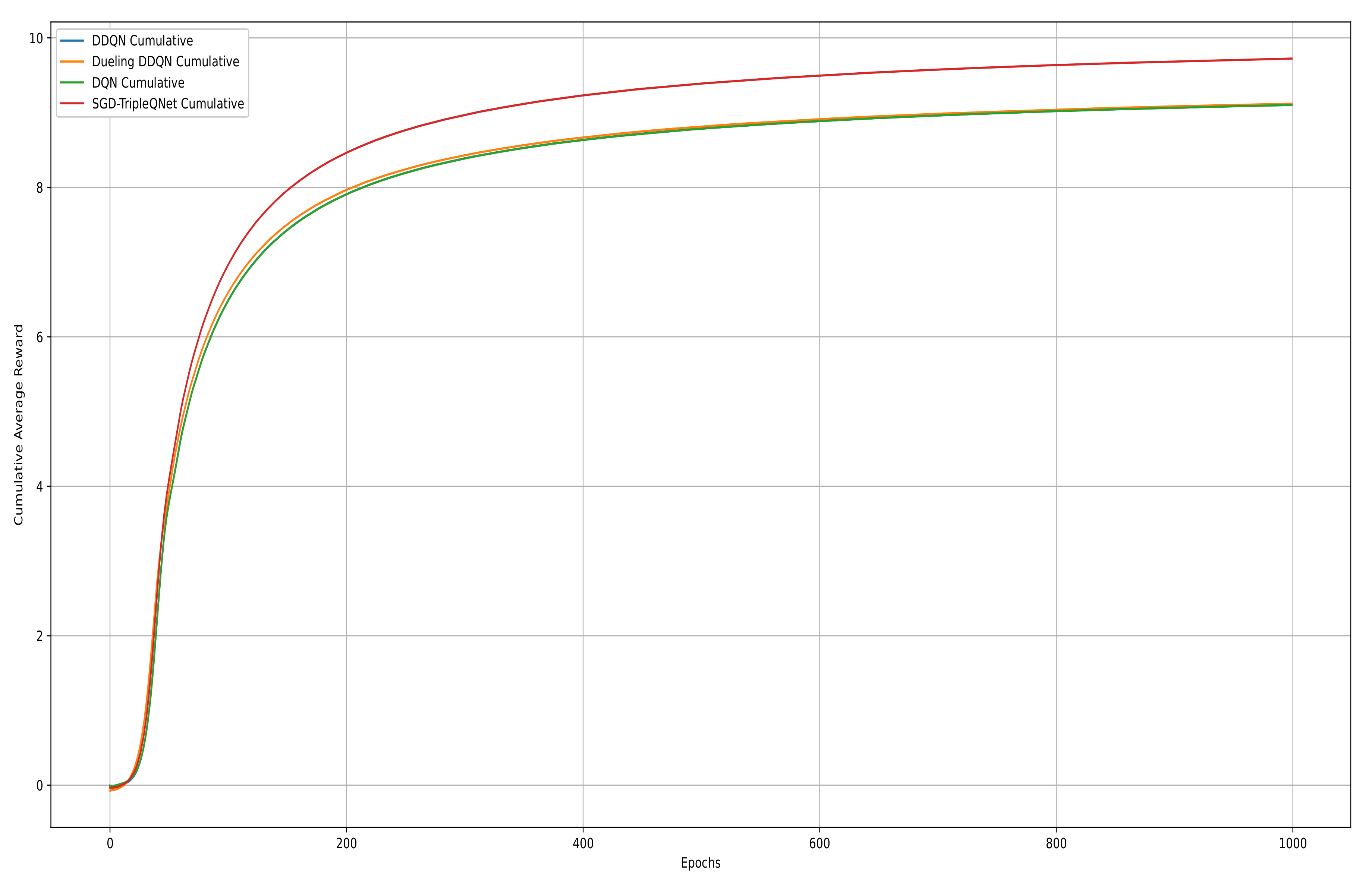
The cumulative average reward curve represents the running average of rewards accumulated over each training epoch, reflecting the model’s long-term learning performance. In Figure 8, we plotted the cumulative average reward curves for DDQN, Dueling DDQN, DQN, and SGD-TripleQNet. Over the first 800 epochs, their performance steadily improves as the models learn. From epochs 800 to 1000, the curves stabilize with minimal fluctuations, indicating that the models have learned a relatively stable strategy. Notably, the SGD-TripleQNet model consistently achieves higher and more stable reward values than the individual models, suggesting that SGD-TripleQNet has the best learning performance.

Figure 8.
Cumulative average reward curves of the DQN, DDQN, Dueling DDQN, and SGD-TripleQNet.
Based on the comprehensive analysis of the average Q-value, average reward curves, and cumulative average reward, SGD-TripleQNet demonstrates clear advantages in terms of convergence speed, decision stability, and generalization. This also confirms that the ensemble deep reinforcement learning strategy not only effectively overcomes the limitations of single models but also validates the effectiveness of dynamic weight adjustment mechanisms in deep reinforcement learning. Furthermore, it provides reliable technical support for the practical application of autonomous driving decision systems. We also recorded the average Q-value, average reward, and cumulative average reward after 1000 epochs in Table 2 below.
Table 2.
The average Q-value, average reward, and cumulative average reward after 1000 epochs.
6. Conclusions
This study proposes an integrated vehicle lane-change decision-making model based on deep reinforcement learning, named SGD-TripleQNet. The model leverages an innovative dynamic weight adjustment mechanism to successfully integrate the complementary advantages of DQN, DDQN, and Dueling DDQN, thereby improving the accuracy and reliability of lane-change decisions while achieving balanced collaboration among the sub-models. Compared to single models, SGD-TripleQNet demonstrates superior performance, addressing common issues of slow convergence and instability in traditional methods. Additionally, the integrated model achieves a good exploration–exploitation balance during the training phase and maintains consistently high performance in later stages. Through the design of a multidimensional reward function that incorporates dynamic safety distance and speed control mechanisms, the model effectively balances efficiency and safety, improving decision-making safety while optimizing travel efficiency.
However, there are limitations to our work that require further improvement. First, the training and inference processes of the integrated model demand significant computational resources. Due to resource constraints, our experiments were conducted on a subset of NGSIM data, which may result in certain limitations in the decision-making outcomes. Second, our research is confined to highway scenarios. The model’s performance in more complex environments, such as intersections, or under extreme conditions like adverse weather, needs further validation to assess its generalizability. Furthermore, the data used in this study are limited to a specific time period during the morning rush hour on a single highway. The lack of data from other time periods, such as nighttime or dusk, restricts the model’s ability to adapt to more diverse real-world traffic conditions. To address these issues, we plan to incorporate a multimodal mechanism and expand the dataset in future work, including more scenarios to enhance the model’s robustness in handling complex and dynamic road environments.
Author Contributions
Methodology, Y.L. and T.Y.; software, J.P. and T.Y.; validation, Y.L. and J.P.; investigation, Y.L., J.P. and T.Y.; data curation, T.Y.; writing—original draft preparation, T.Y.; writing—review and editing, Y.L. and T.Y.; visualization, T.Y., J.P. and L.T.; funding acquisition, Y.L. and L.T. All authors have read and agreed to the published version of the manuscript.
Funding
This research was supported by the “Research and Development of Data Security Sharing, Integration and Situational Awareness System Based on Quantum Blockchain Vehicular Networking” as a “2023 Liaoning Province Unveiling the List of Commanders” Science and Technology Program Project (Technology Tackling Category)–(2023JH1/10400099).
Data Availability Statement
The raw data supporting the conclusions of this article will be made available by the authors on request.
Acknowledgments
The authors would like to express their gratitude for the financial support from the Liaoning Provincial Science and Technology Program “Listed and Commanding”.
Conflicts of Interest
The authors declare no conflicts of interest.
References
- Liu, T.; Tang, X.; Wang, H.; Zhang, M.; Huang, H. Dynamic States Prediction in Autonomous Vehicles: Comparison of Three Different Methods. IEEE Intell. Transp. Syst. Conf. (ITSC) 2019, 2019, 3750–3755. [Google Scholar]
- Gao, F.; Zheng, X.; Hu, Q.; Liu, H. Integrated Decision and Motion Planning for Highways with Multiple Objects Using a Naturalistic Driving Study. Sensors 2025, 25, 26. [Google Scholar] [CrossRef]
- Ko, W.; Shim, M.; Park, S.; Lee, S.; Yun, I. Development of Test Cases for Automated Vehicle Driving Safety Assessment Using Driving Trajectories. Sensors 2024, 24, 7981. [Google Scholar] [CrossRef] [PubMed]
- Yang, Z.; Gao, Z.; Gao, F.; Wu, X.; He, L. Lane changing assistance strategy based on an improved probabilistic model of dynamic occupancy grids. Front. Inf. Technol. Electron. Eng. 2021, 22, 1492–1504. [Google Scholar] [CrossRef]
- Cesari, G.; Schildbach, G.; Carvalho, A.; Borrelli, F. Scenario model predictive control for lane change assistance and autonomous driving on highways. IEEE Intell. Transp. Syst. Mag. 2017, 9, 23–35. [Google Scholar] [CrossRef]
- He, Y.; Feng, J.; Wei, K.; Cao, J.; Chen, S.; Wan, Y. Modeling and simulation of lane-changing and collision avoiding autonomous vehicles on superhighways. Phys. A Stat. Mech. Its Appl. 2023, 609, 128328. [Google Scholar] [CrossRef]
- Liu, S.; Wang, X.; Hassanin, O.; Xu, X.; Yang, M.; Hurwitz, D.; Wu, X. Calibration and evaluation of responsibility-sensitive safety (RSS) in automated vehicle performance during cut-in scenarios. Transp. Res. Part C Emerg. Technol. 2021, 125, 103037. [Google Scholar] [CrossRef]
- Moon, H.; Kang, S.H.; Eom, J.; Hwang, M.J.; Kim, Y.; Wang, J.; Kim, B.; Kim, T.; Ga, T.; Choi, J.; et al. Autonomous Robot Racing Competitions: Truly Multivehicle Autonomous Racing Competitions [Competitions]. IEEE Robot. Autom. Mag. 2024, 31, 123–132. [Google Scholar] [CrossRef]
- Selvi, V.T.; Dhurgadevi, M.; Prithiviraj, P.; Jackulin, T.; Baskaran, K. Extending the FSM Model for Critical Decision-Making and Safety Control in Autonomous Vehicles. Int. J. Intell. Syst. Appl. Eng. 2024, 12, 397–410. [Google Scholar]
- Tang, T.; Guo, Y.; Souders, D.J.; Li, X.; Yang, M.; Xu, X.; Qian, X. Moderating effects of policy measures on intention to adopt autonomous vehicles: Evidence from China. Travel Behav. Soc. 2024, 38, 100921. [Google Scholar] [CrossRef]
- Chen, Z.; Wang, Y.; Hu, H.; Zhang, Z.; Zhang, C.; Zhou, S. Investigating Autonomous Vehicle Driving Strategies in Highway Ramp Merging Zones. Mathematics 2024, 12, 3859. [Google Scholar] [CrossRef]
- Li, H.; Zhang, S. Lane change behavior with uncertainty and fuzziness for human driving vehicles and its simulation in mixed traffic. Phys. A Stat. Mech. Its Appl. 2022, 606, 128130. [Google Scholar] [CrossRef]
- Gao, L.; Tang, F.; Guo, P.; He, J. Research on Improved LQR Control for Self-driving Vehicle Lateral Motion. Mech. Sci. Technol. Aerosp. Eng. 2021, 40, 435–441. [Google Scholar]
- Van Hoek, R.; Ploeg, J.; Nijmeijer, H. Cooperative driving of automated vehicles using B-splines for trajectory planning. IEEE Trans. Intell. Veh. 2021, 6, 594–604. [Google Scholar] [CrossRef]
- Erke, S.; Dai, B.; Nie, Y.; Zhu, Q.; Xiao, L.; Zhao, D. An improved A-Star based path planning algorithm for autonomous land vehicles. Int. J. Adv. Robot. Syst. 2020, 17, 1729881420962263. [Google Scholar] [CrossRef]
- Moghadam, M.; Elkaim, G.H. A hierarchical architecture for sequential decision-making in autonomous driving using deep reinforcement learning. arXiv 2019, arXiv:1906.08464. [Google Scholar]
- Kiran, B.R.; Sobh, I.; Talpaert, V.; Mannion, P.; Perez, P. Deep reinforcement learning for autonomous driving: A survey. IEEE Trans. Intell. Transp. Syst. 2021, 10, 1–18. [Google Scholar] [CrossRef]
- Mnih, V.; Koray, K.; David, S.; Alex, G.; Ioannis, A.; Daan, W. Playing Atari with Deep Reinforce-ment Learning. arXiv 2013, arXiv:1312.5602. [Google Scholar]
- Qiao, L.; Bao, H.; Xuan, Z.; Liang, J.; Pan, F. Autonomous Driving Ramp Merging Model Based on Reinforcement Learning. Comput. Eng. 2018, 44, 20–24. [Google Scholar]
- Shen, Y.; Peng, J.; Kang, C.; Zhang, S.; Yi, F.; Wan, J.; Wang, X. Collaborative optimisation of lane change decision and trajectory based on double-layer deep reinforcement learning. Int. J. Veh. Des. 2023, 92, 336–356. [Google Scholar] [CrossRef]
- Lv, K.; Pei, X.; Chen, C.; Xu, J. A Safe and Efficient Lane Change Decision-Making Strategy of Autonomous Driving Based on Deep Reinforcement Learning. Mathematics 2022, 10, 1551. [Google Scholar] [CrossRef]
- Yang, Z.; Wu, Z.; Wang, Y.; Wu, H. A Deep Reinforcement Learning Lane-Changing Decision Algorithm for Intelligent Vehicles Combining LSTM Trajectory Prediction. World Electr. Veh. J. 2024, 15, 173. [Google Scholar] [CrossRef]
- Deva Hema, D.; Rajeeth Jaison, T. A Novel Deep Learning-Driven Smart System for Lane Change Decision-Making. Int. J. Intell. Transp. Syst. Res. 2024, 22, 648–659. [Google Scholar]
- An, H.; Jung, J. A Novel Decision-Making System for Lane Change Using Deep Reinforcement Learning in Connected and Automated Driving. Electronics 2019, 8, 542. [Google Scholar] [CrossRef]
- Zhang, X.; Wu, L. Behavior decision-making model for autonomous vehicles based on an ensemble deep reinforcement learning. Automot. Saf. Energy 2023, 14, 472–479. [Google Scholar]
- Ahmed, I. Characterizing lane changing behavior and identifying extreme lane changing traits. Transp. Lett. 2023, 15, 450–464. [Google Scholar] [CrossRef]
- Xu, Z. Analytical study of the lane-by-lane variation for lane-utility and traffic safety performance assessment using NGSIM data. MATEC Web Conf. 2017, 124, 04001. [Google Scholar] [CrossRef]
- Lu, X.; Varaiya, P.; Horowitz, R. Fundamental Diagram Modelling and Analysis Based NGSIM Data. IFAC Proc. 2009, 42, 367–374. [Google Scholar] [CrossRef]
- Lu, J. State of charge estimation for energy storage lithium-ion batteries based on gated recurrent unit neural network and adaptive Savitzky-Golay filter. Ionics 2024, 30, 297–310. [Google Scholar] [CrossRef]
- Li, H.; Gao, D.; Shi, L.R. State of Health Estimation of Lithium-Ion Battery Using Multi-Health Features Based on Savitzky–Golay Filter and Fitness-Distance Balance- and Lévy Roulette-Enhanced Coyote Optimization Algorithm-Optimized Long Short-Term Memory. Processes 2024, 12, 2284. [Google Scholar] [CrossRef]
- Nadia, K.; Farinawati, Y.; Rohaya, W.R. Chemometrics analysis for the detection of dental caries via UV absorption spectroscopy. Spectrochim. Acta Part A Mol. Biomol. Spectrosc. 2022, 266, 120464. [Google Scholar]
- Kordestani, H.; Zhang, C. Direct Use of the Savitzky–Golay Filter to Develop an Output-Only Trend Line-Based Damage Detection Method. Sensors 1983, 20, 1983. [Google Scholar] [CrossRef] [PubMed]
- Mukadam, M.; Akansel, C.; Alireza, N. Tactical Decision Making for Lane Changing with Deep Reinforcement Learning. Comput. Sci. 2017, 302, 248. [Google Scholar]
- Azar, A.T.; Koubaa, A.; Ali Mohamed, N.; Ibrahim, H.A.; Ibrahim, Z.F.; Kazim, M.; Ammar, A.; Benjdira, B.; Khamis, A.M.; Hameed, I.A.; et al. Drone Deep Reinforcement Learning: A Review. Electronics 2021, 10, 999. [Google Scholar] [CrossRef]
- Zheng, L.; Liu, W.; Zhai, C. A Dynamic Lane-Changing Trajectory Planning Algorithm for Intelligent Connected Vehicles Based on Modified Driving Risk Field Model. Actuators 2024, 13, 380. [Google Scholar] [CrossRef]
- Tang, L.; Niu, Y.; Wang, R.; Xing, B.; Wang, Y. Classification study of interpretable methods for reinforcement learning. Appl. Res. Comput. 2023, 41, 1001–3695. [Google Scholar]
- Shi, H.; Chen, J.; Zhang, F.; Liu, M.; Zhou, M. Achieving Robust Learning Outcomes in Autonomous Driving with DynamicNoise Integration in Deep Reinforcement Learning. Drones 2024, 8, 470. [Google Scholar] [CrossRef]
- Hussain, Q.; Dias, C.; Al-Shahrani, A.; Hussain, I. Safety Analysis of Merging Vehicles Based on the Speed Difference between on-Ramp and Following Mainstream Vehicles Using NGSIM Data. Sustainability 2022, 24, 16436. [Google Scholar] [CrossRef]

Disclaimer/Publisher’s Note: The statements, opinions and data contained in all publications are solely those of the individual author(s) and contributor(s) and not of MDPI and/or the editor(s). MDPI and/or the editor(s) disclaim responsibility for any injury to people or property resulting from any ideas, methods, instructions or products referred to in the content. |
© 2025 by the authors. Licensee MDPI, Basel, Switzerland. This article is an open access article distributed under the terms and conditions of the Creative Commons Attribution (CC BY) license (https://creativecommons.org/licenses/by/4.0/).