Article

The Multi-Soliton Solutions for the (2+1)-Dimensional Caudrey–Dodd–Gibbon–Kotera–Sawada Equation

1
Department of Mathematics, Lishui University, Lishui 323000, China
2
Department of Mathematics, Zhejiang Sci-Tech University, Hangzhou 310018, China
3
Department of Photoelectric Engineering, Lishui University, Lishui 323000, China
*
Author to whom correspondence should be addressed.
Mathematics 2025, 13(2), 236; https://doi.org/10.3390/math13020236
Submission received: 29 November 2024 / Revised: 27 December 2024 / Accepted: 8 January 2025 / Published: 12 January 2025

Abstract

:
The (2+1)-dimensional integrable Caudrey–Dodd–Gibbon–Kotera–Sawada equation is a higher-order generalization of the Kadomtsev–Petviashvili equation, which can be applied in some physical branches such as the nonlinear dispersive phenomenon. In this paper, we first present the bilinear form for this equation after constructing one Bäcklund transformation. As a result, the one-soliton solution, two-soliton solution, and three-soliton solution are shown successively and the corresponding soliton structures are constructed. These solitons and their interactions illustrate that the obtained solutions have powerful applications.

1. Introduction

Konpelchenko and Dubrovsky first proposed the following (2+1)-dimensional Caudrey–Dodd–Gibbon–Kotera–Sawada (CDGKS) equation:
36 u t + ( u 4 x + 15 u u x x + 15 u 3 ) x 5 ( u x x y + 3 u u y + 3 u x v y + v y y ) , u = v x ,
through the inverse scattering transform method, in which u = u ( x , y , t ) , v = v ( x , y , t ) [1]. Cheng proved that this (2+1)-dimensional equation can be constrained to the integrable hierarchies in 1+1 dimensions [2]. Hu proposed a hierarchy of the bilinear CDGKS equations with a unified structure and proved one nonlinear superposition formula under certain conditions [3]. For the CDGKS Equation (1), Cao obtained the quasi-periodic solutions in terms of the Riemann theta functions [4,5]. Tang illustrated the lump solitons and their interaction phenomena through a direct method [6], while Peng studied the characteristics of the solitary waves and lump waves with interaction phenomena by the way of vector notations [7]. Fang demonstrated the lump-type solution, rogue wave, fusion and fission phenomena by means of the Hirota direct method, and symbolic computation [8]. Zhang constructed the generalized lump solution, classical lump solution, and the novel analytical solution based on the bilinear neural network method [9]. Ma and Zhuang presented the specific expression of the N-soliton solutions for the (2+1)-dimensional generalized CDGKS equation in fluid mechanics under Hirota’s bilinear method and studied the different localized waves [10,11,12]. The Nth-order Pfaffian solutions via the modified Pfaffian technique, the symmetry group theorem by using the improved Clarkson, and the Kruskal (CK) method were also applied to the above equation [13,14]. The Kadomtsev–Petviashvili (KP) equation corresponds to a third-order Korteweg-de Vries (KdV) integrable equation, while the CDGKS equation is the fifth-order modified KdV integrable equation, which is a higher-order representation of the KP equation [2,15].
We know that to find the solitary waves and solitons for an integrable system, apart from the above-mentioned methods, such as the Hirota bilinear method, the Bäcklund transformation, the direct CK’s method, and the bilinear neural network method, there are still some powerful tools that can be listed, including the inverse scattering method, the Darboux transformation, the Painlevé analysis approach, and the bilinear residual network method [16,17,18,19,20,21,22].
The paper is outlined as follows: In Section 2, the bilinear form is written through a Bäcklund transformation for Equation (1). Therefore, the solutions which contain multi-solitons exist for this equation. The abundant solitons, such as the peak, plateau, M-type, and molecular solitons for the one-soliton solution, the interactions of two peak solitons, two M-type solitons, and two molecular solitons, as well as breathers with their molecules for the two-soliton solution, the interactions of three peak solitons, three molecular solitons, one peak soliton, and a breather for the three-soliton solution are all constructed successively after the constrained parameters are taken suitably. Section 3 is a short summary.

2. The Multi-Soliton Solutions and Their Hybrid Structures

We introduce the following Bäcklund transformation of Equation (1):
u = 2 ( ln f ) x x , v = 2 ( ln f ) x ,
with the transformation function f = f ( x , y , t ) being defined later. Therefore, Equation (1) has the bilinear form
( 36 D x D t + D x 6 5 D x 3 D y 5 D y 2 ) ( f · f ) = 0 ,
where the Hirota derivative operators are as follows [23,24]:
D x U D y V D t W ( P · Q ) = ( x x ) U ( y y ) V ( t t ) W P ( x , y , t ) · Q ( x , y , t ) | x = x , y = y , t = t .
In a similar situation, Equation (3) has another bilinear version as follows:
36 f x f t 36 f x t f f 6 x f + 6 f 5 x f x 15 f 4 x f x x
+ 10 f 3 x 2 5 f 3 x f y + 5 f 3 x y f + 15 f x x f x y 15 f x x y f x + 5 f y y f 5 f y 2 = 0 .

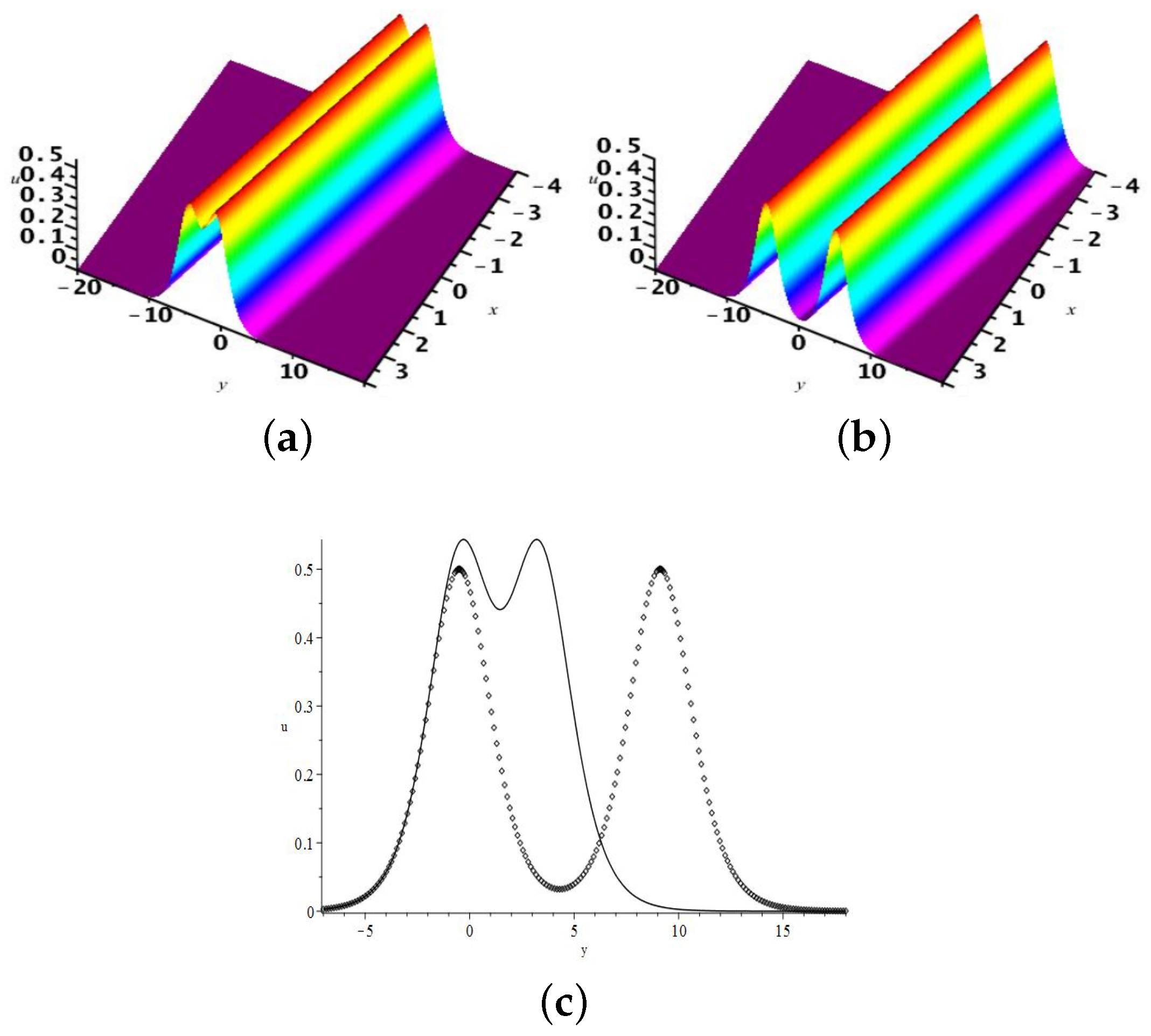
2.1. The One-Soliton Solution

Equation (1) has a single soliton solution through Equation (2) with
u = 2 k 1 2 ( b 1 e ξ 1 + 4 δ 1 e 2 ξ 1 + b 1 δ 1 e 3 ξ 1 ) f 2 , v = 2 k 1 ( b 1 e ξ 1 + 2 δ 1 e 2 ξ 1 ) f ,
where
f f 1 = 1 + b 1 e ξ 1 + δ 1 e 2 ξ 1 , ξ 1 = k 1 x + k 1 3 y + 1 4 k 1 5 t ,
Here, k 1 , b 1 and δ 1 are three constants. In fact, the parameter δ 1 affects the structure of this soliton through its determined function f. For example, the single peak soliton can be presented when δ 1 = 1 4 . As the value of δ 1 decreases, the shape of the soliton is changed. Figure 1 and Figure 2 show the evolution process with δ 1 = 1 4 , 1 16 , 1 50 , and 1 15 , 000 , respectively, with other parameters taking the same value k 1 = b 1 = 1 when t = 2 . As a result, the peak soliton (Figure 1a), plateau soliton (Figure 1b), M-type soliton (Figure 2a), and molecular soliton (Figure 2b) will be constructed sooner or later.

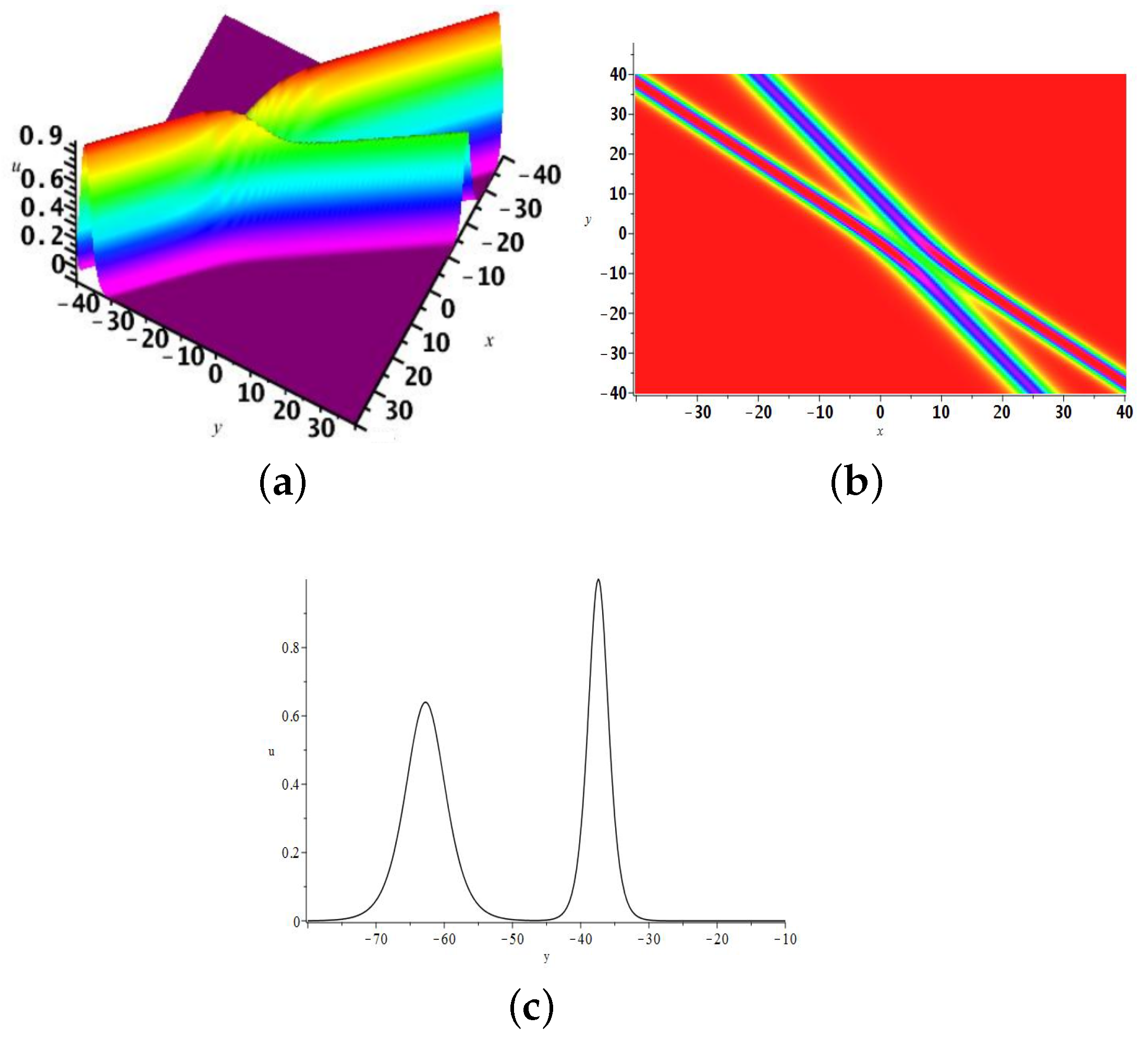
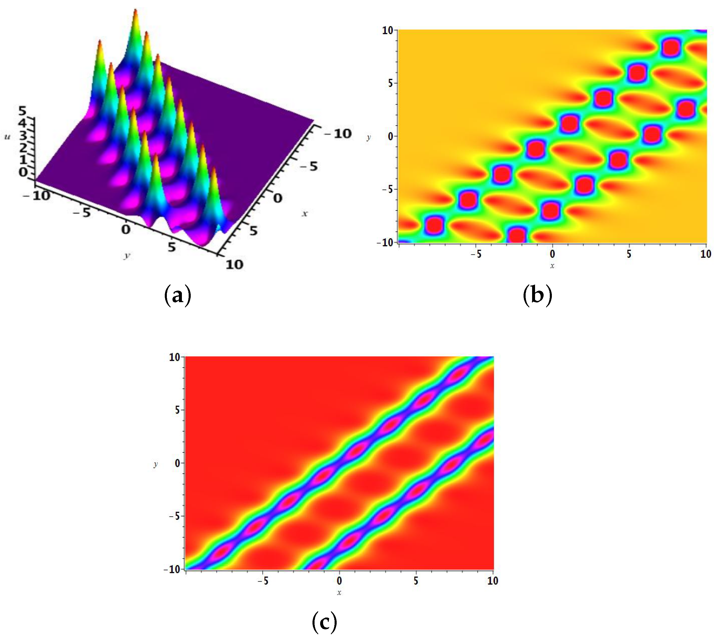
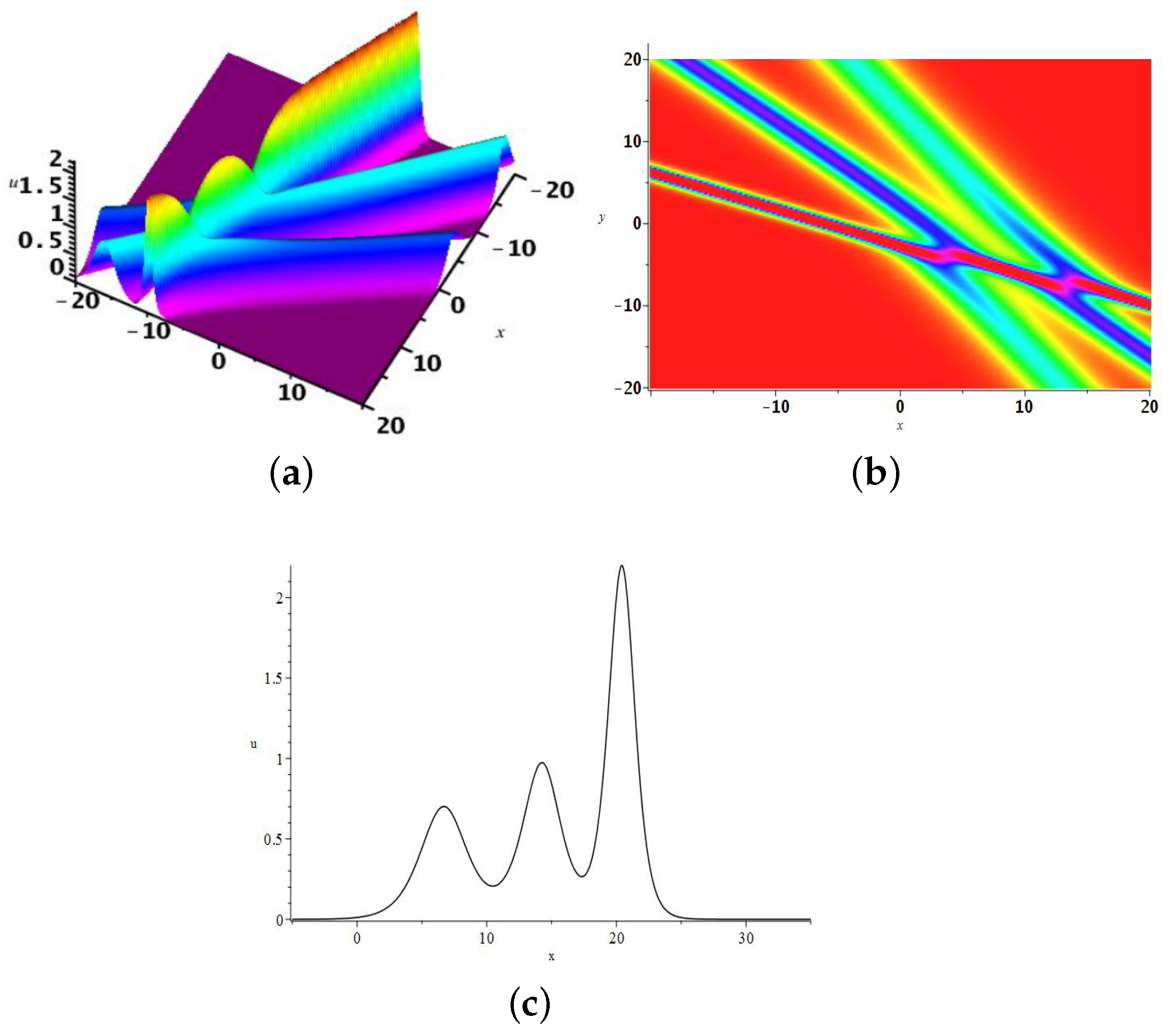
2.2. The Two-Soliton Solution

The two-soliton solution of Equation (1) can be expressed through Equation (2):
f f 2 = 1 + b 1 e ξ 1 + b 2 e ξ 2 + δ 1 e 2 ξ 1 + δ 2 e 2 ξ 2 + B 12 e ξ 1 + ξ 2
+ b 1 δ 2 a 12 2 e ξ 1 + 2 ξ 2 + b 2 δ 1 a 12 2 e 2 ξ 1 + ξ 2 + Y 12 e 2 ξ 1 + 2 ξ 2 , ξ 1 = k 1 x + k 1 3 y + 1 4 k 1 5 t , ξ 2 = k 2 x + k 2 3 y + 1 4 k 2 5 t ,
where the constraint constants have
a 12 = k 1 k 2 k 1 + k 2 , Y 12 = δ 1 δ 2 a 12 4 ,
from Equation (5).
For this circumstance, to study the soliton structures for the CDGKS Equation (1) through the auxiliary function of Equation (8), the asymptotic analysis technique should be adopted [25,26,27,28]. That is, when taking the independent parameters B 12 = b 1 = b 2 = k 1 = 1 and k 2 = 4 5 , the asymptotic expressions have the following forms:
(1) Before the action ( t ) ,
(a) ξ 1 0 , ξ 2 + , f b 2 e ξ 2 + δ 2 e 2 ξ 2 + B 12 e ξ 1 + ξ 2 + δ 1 b 2 a 12 2 e 2 ξ 1 + ξ 2 + δ 2 b 1 a 12 2 e ξ 1 + 2 ξ 2 + Y 12 e 2 ξ 1 + 2 ξ 2 ,
u u 1 = 2 ( 1076168025 e ξ 10 + 2 ξ 20 + 656100 δ 1 e 2 ξ 10 + 2 ξ 20 + 164025 δ 1 e 3 ξ 10 + 2 ξ 20 + 688747536 δ 2 e 3 ξ 20
+ 43578162 δ 2 e ξ 10 + 3 ξ 20 + 104976 δ 2 e 2 ξ 10 + 3 ξ 20 + 1522152 δ 1 δ 2 e 2 ξ 10 + 3 ξ 20 + 531442 δ 1 δ 2 e 3 ξ 10 + 3 ξ 20
+ 164025 δ 2 2 e ξ 10 + 4 ξ 20 + 16 δ 1 2 δ 2 e 4 ξ 10 + 3 ξ 20 + 656100 δ 1 δ 2 2 e 2 ξ 10 + 4 ξ 20 + 25 δ 1 δ 2 2 e 3 ξ 10 + 4 ξ 20 ) / 25 ( 6561 e ξ 20
+ 6561 e ξ 10 + ξ 20 + δ 1 e 2 ξ 10 + ξ 20 + δ 2 e ξ 10 + 2 ξ 20 + 6561 δ 2 e 2 ξ 20 + δ 1 δ 2 e 2 ξ 10 + 2 ξ 20 ) 2 ,
(b) ξ 2 0 , ξ 1 , f 1 + b 2 e ξ 2 + δ 2 e 2 ξ 2 ,
u u 2 = 32 ( 1 + 4 δ 2 e ξ 20 + δ 2 e 2 ξ 20 ) e ξ 20 25 ( 1 + e ξ 20 + δ 2 e 2 ξ 20 ) 2 .
(2) After the action ( t + ) ,
(a) ξ 1 0 , ξ 2 , f 1 + b 1 e ξ 1 + δ 1 e 2 ξ 1 ,
u u 1 + = 2 ( 1 + 4 δ 1 e ξ 10 + δ 1 e 2 ξ 10 ) e ξ 10 ( 1 + e ξ 10 + δ 1 e 2 ξ 10 ) 2 ,
(b) ξ 2 0 , ξ 1 + , f b 1 e ξ 1 + δ 1 e 2 ξ 1 + B 12 e ξ 1 + ξ 2 + δ 1 b 2 a 12 2 e 2 ξ 1 + ξ 2 + δ 2 b 1 a 12 2 e ξ 1 + 2 ξ 2 + Y 12 e 2 ξ 1 + 2 ξ 2 ,
u u 2 + = 2 ( 688747536 e 2 ξ 10 + ξ 20 + 1076168025 δ 1 e 3 ξ 10 + 43578162 δ 1 e 3 ξ 10 + ξ 20 + 164025 δ 1 e 3 ξ 10 + 2 ξ 20
+ 419904 δ 2 e 2 ξ 10 + 2 ξ 20 + 104976 δ 2 e 2 ξ 10 + 3 ξ 20 + 104976 δ 1 2 e 4 ξ 10 + ξ 20 + 1167858 δ 1 δ 2 e 3 ξ 10 + 2 ξ 20
+ 531442 δ 1 δ 2 e 3 ξ 10 + 3 ξ 20 + 419904 δ 1 2 δ 2 e 4 ξ 10 + 2 ξ 20 + 16 δ 1 2 δ 2 e 4 ξ 10 + 3 ξ 20 + 25 δ 1 δ 2 2 e 3 ξ 10 + 4 ξ 20 ) / 25 ( 6561 e ξ 10
+ 6561 e ξ 10 + ξ 20 + δ 1 e 2 ξ 10 + ξ 20 + δ 2 e ξ 10 + 2 ξ 20 + 6561 δ 1 e 2 ξ 10 + δ 1 δ 2 e 2 ξ 10 + 2 ξ 20 ) 2 .
Here, ξ 10 = x + y + 1 4 t , ξ 20 = 4 5 x + 64 125 y + 256 3125 t .
In order to describe the soliton solution u of Equation (1) with Equation (8), we just focus on the parameters δ 1 and δ 2 , while the others are fixed; that is, the independent parameters B 12 = b 1 = b 2 = k 1 = 1 and k 2 = 4 5 are taken as above. For this time, two separated solitary waves of the solution u will interplay with each other as the time increases. However, they maintain the original styles after their interactions. That is, two solitons have not changed their shapes, velocities, and amplitudes, although their phases and positions shift with the varying time. Figure 3, Figure 4 and Figure 5 show the elastic interactions of two peak solitons, two M-type solitons, and two molecular solitons with δ 1 = δ 2 = 1 4 , 1 150 , and 1 15 , 000 , respectively ( t = 10 ) . These plots show that the soliton structures change with the varying parameters δ 1 and δ 2 .
We know that the breather is a periodic structure in a certain direction, but also a partially localized breathing wave. In order to derive the breather solution for the solution u of Equation (1) with Equation (8), we establish the following conjugate relation for the related parameters ( I is a imaginary unit) [29,30,31,32]:
b 1 = b 2 ¯ = b 11 + b 22 I , k 1 = k 2 ¯ = k + κ I , δ 1 = δ 2 ¯ = σ + ρ I ,
while the others satisfy a 12 = k 1 k 2 k 1 + k 2 , Y 12 = δ 1 δ 2 a 12 4 . Therefore,
f f 2 = 1 + 2 b 1 cos ( Ξ ) e Ω + [ B 12 2 ρ sin ( 2 Ξ ) + 2 σ cos ( 2 Ξ ) ] e 2 Ω
+ 2 b 1 κ 2 [ ρ sin ( Ξ ) σ cos ( Ξ ) ] e 3 Ω k 2 + κ 4 ( ρ 2 + σ 2 ) e 4 Ω k 4 , ξ 1 = Ξ I + Ω , ξ 2 = Ξ I + Ω ,
with
Ξ = κ x + κ ( 3 k 2 κ 2 ) y + 1 4 κ ( κ 4 10 k 2 κ 2 + 5 k 4 ) t , Ω = k x + k ( k 2 3 κ 2 ) y + 1 4 k ( k 4 10 k 2 κ 2 + 5 κ 4 ) t ,
from Equation (8).
This transformation function can induce the breather structure for the solution u through Equation (2). For example, two kinds of breathers for the solution u of Equation (1) with Equation (15) are presented, when B 12 = k = 1 , κ = 4 5 , σ = ρ = 1 5 , t = 0 , but b 1 = b 2 = 1 or b 1 = b 2 = 1 10 (Figure 6). As the value of b 1 and b 2 varies, the breathers show different structures. Furthermore, when the module of | δ 1 | and | δ 1 |   1 16 , the breather molecules for the solution u of Equation (1) with Equation (15) can be constructed. Figure 7 owns two kinds of breather molecules, when B 12 = k = 1 , κ = 4 5 , t = 0 , but also when b 1 = b 2 = 1 2 , σ = ρ = 1 500 , or b 1 = b 2 = 1 10 , σ = ρ = 1 1500 . To a certain extent, this phenomenon shows that as the values of related parameters decrease, the distance between two lines of periodic solitons becomes larger and the breather molecule changes increasingly noticeably.

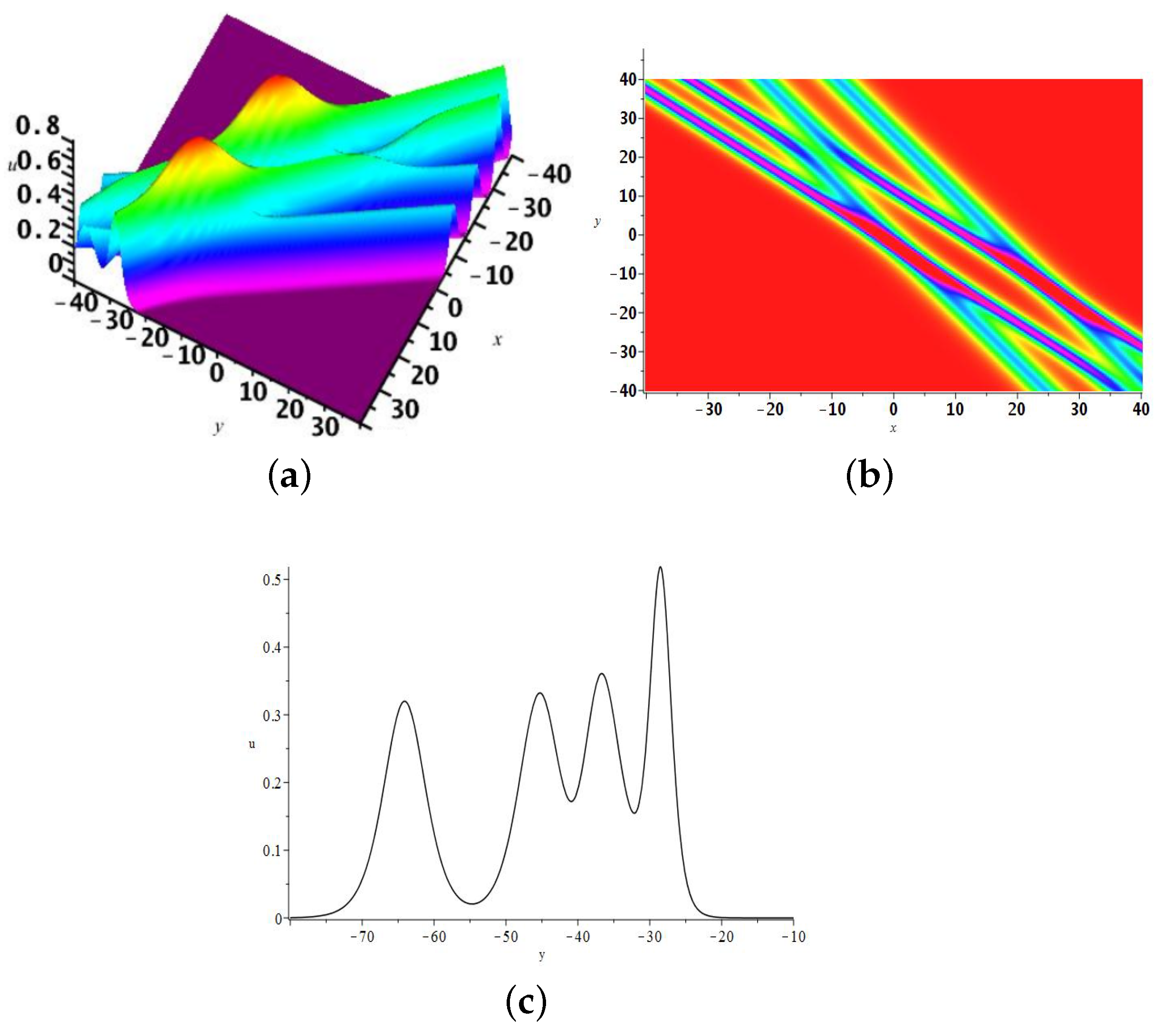
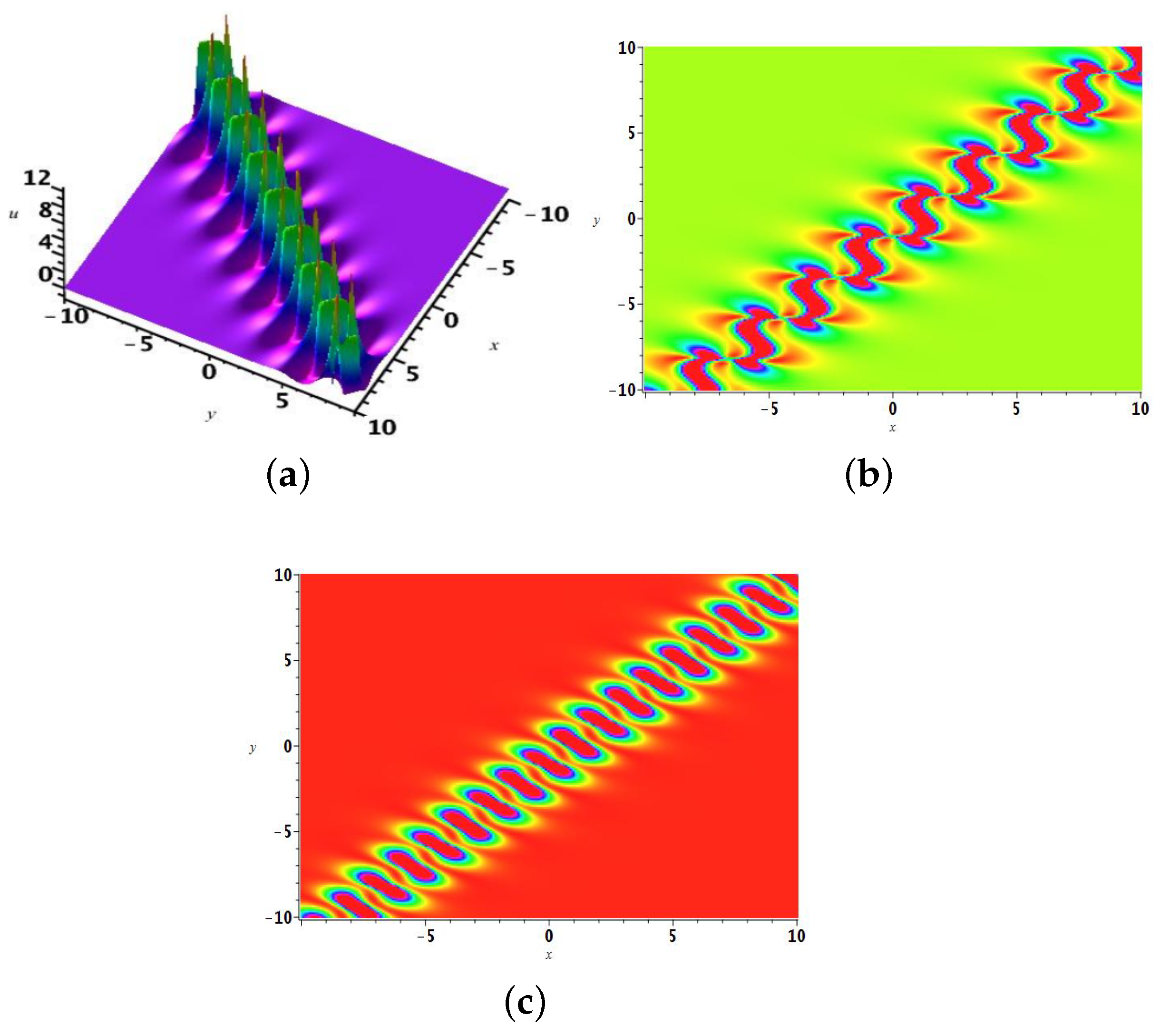
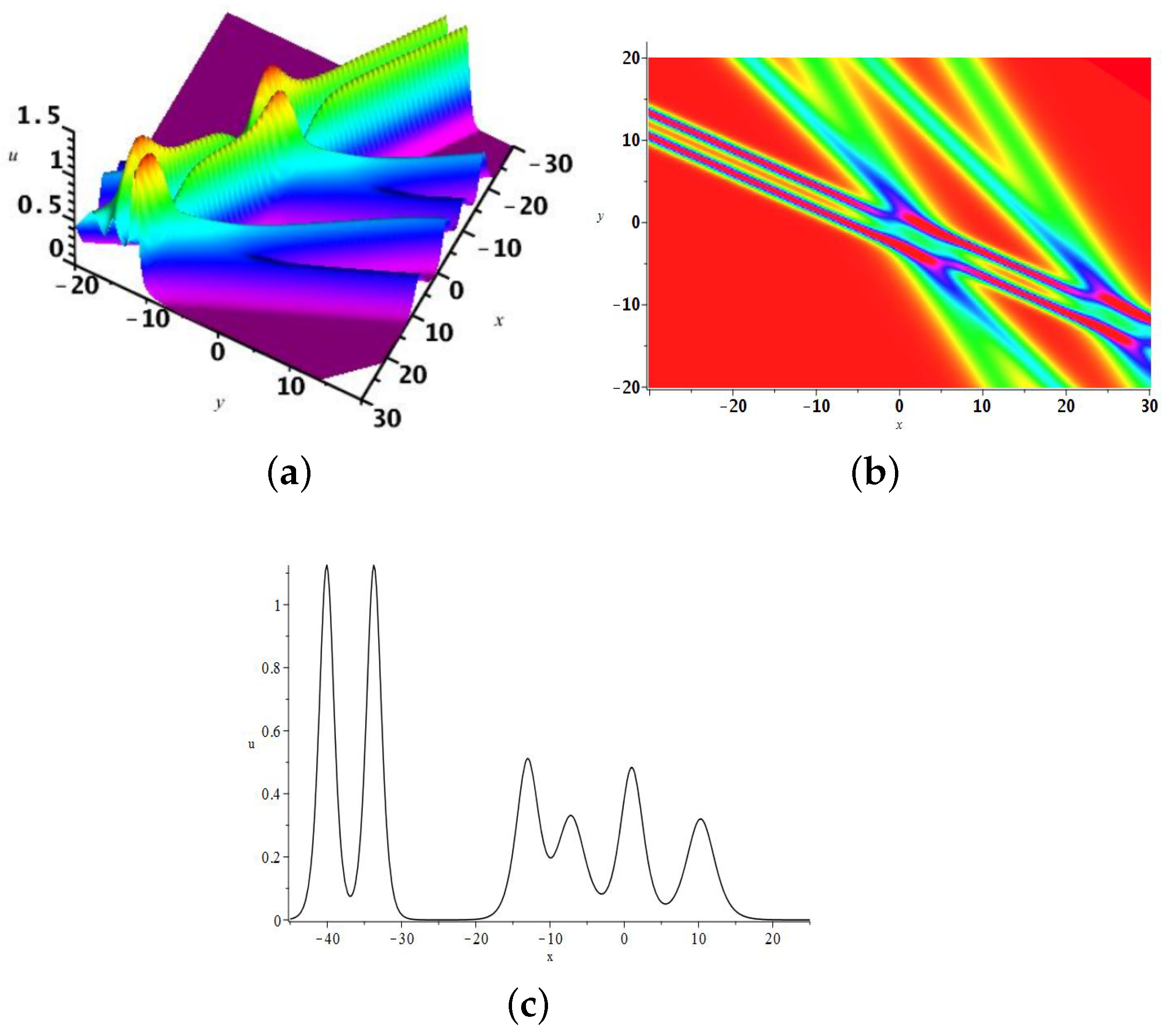
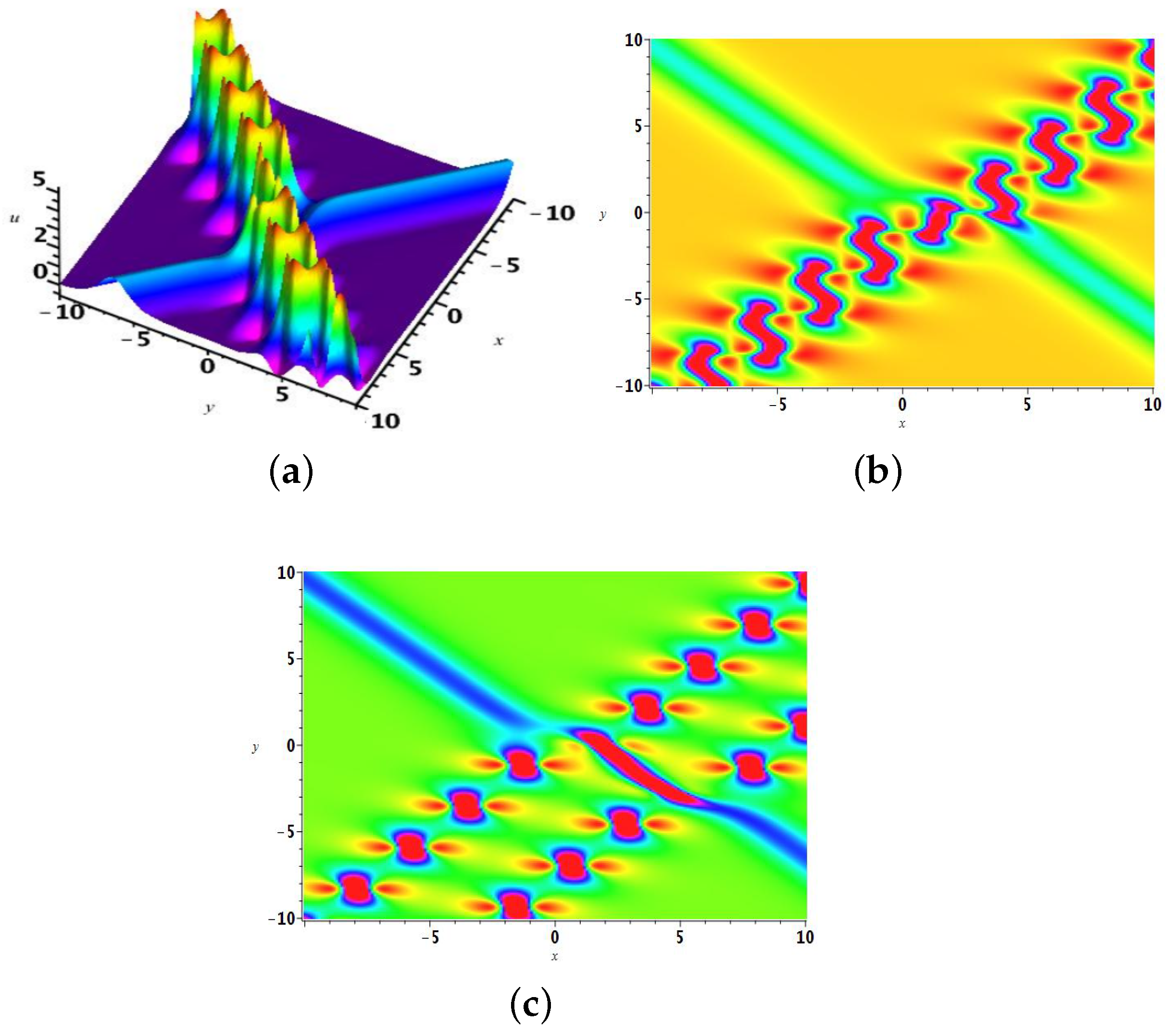
2.3. The 3-Soliton Solution

In order to derive the interaction solution of three solitons for Equation (1), we devise the auxiliary function f as follows:
f f 3 = 1 + b 1 e ξ 1 + b 2 e ξ 2 + b 3 e ξ 3 + δ 1 e 2 ξ 1 + δ 2 e 2 ξ 2 + δ 3 e 2 ξ 3 + B 12 e ξ 1 + ξ 2 + B 13 e ξ 1 + ξ 3 + B 23 e ξ 2 + ξ 3
+ Y 12 e 2 ξ 1 + 2 ξ 2 + Y 13 e 2 ξ 1 + 2 ξ 3 + Y 23 e 2 ξ 2 + 2 ξ 3 + Y 123 e 2 ξ 1 + 2 ξ 2 + 2 ξ 3 + δ 1 b 2 a 12 2 e 2 ξ 1 + ξ 2 + δ 1 b 3 a 13 2 e 2 ξ 1 + ξ 3
+ δ 2 b 1 a 12 2 e ξ 1 + 2 ξ 2 + δ 2 b 3 a 23 2 e 2 ξ 2 + ξ 3 + δ 3 b 1 a 13 2 e ξ 1 + 2 ξ 3 + δ 3 b 2 a 23 2 e ξ 2 + 2 ξ 3 + a 12 a 13 a 23 B 123 e ξ 1 + ξ 2 + ξ 3
+ δ 1 a 12 2 a 13 2 B 23 e 2 ξ 1 + ξ 2 + ξ 3 + δ 2 a 12 2 a 23 2 B 13 e ξ 1 + 2 ξ 2 + ξ 3 + δ 3 a 13 2 a 23 2 B 12 e ξ 1 + ξ 2 + 2 ξ 3
+ b 1 a 12 2 a 13 2 Y 23 e ξ 1 + 2 ξ 2 + 2 ξ 3 + b 2 a 12 2 a 23 2 Y 13 e 2 ξ 1 + ξ 2 + 2 ξ 3 + b 3 a 13 2 a 23 2 Y 12 e 2 ξ 1 + 2 ξ 2 + ξ 3 ,
where ξ i = k i x + k i 3 y + 1 4 k i 5 t ( i = 1 , 2 , 3 ) .
Therefore, the constraint constants satisfy
a i j = k i k j k i + k j , Y i j = δ i δ j a i j 4 ( 1 i < j 3 ) ,
Y 123 = Y 12 Y 13 Y 23 δ 1 δ 2 δ 3 , B 123 = b 3 B 12 a 12 b 2 B 13 a 13 + b 1 B 23 a 23 ,
from the bilinear Equation (5).
To illustrate the effect of Equation (17), one can choose the independent parameters as
B 12 = B 13 = B 23 = b 1 = b 2 = b 3 = k 1 = 1 , k 2 = 4 5 , k 3 = 3 2 ,
then the expected solitons can be derived from Equation (2) through Equation (17) with Equations (18) and (19) ( δ i ( i = 1 , 2 , 3 ) will be suitable taken). Figure 8 and Figure 9 are two typical structures for this situation ( t = 5 ) . Figure 8 shows the interaction of three peak solitons, while Figure 9 presents the interaction of three molecular solitons, when δ i ( i = 1 , 2 , 3 ) = 1 4 and 1 14 , 000 , respectively.
Finally, after the established conjugate relations for the related parameters are
b 1 = b 2 ¯ = b 11 + b 22 I , k 1 = k 2 ¯ = k + κ I , δ 1 = δ 2 ¯ = σ + ρ I , a 12 = A 12 I ,
a 13 = a 23 ¯ = A 13 + A 23 I , Y 12 = y 12 , Y 13 = Y 23 ¯ = y 13 + y 23 I , B 13 = B 23 ¯ = b 13 + b 23 I ,
that is
a 12 = κ I k , a 13 = k k 3 + κ I k + k 3 + κ I , a 23 = k k 3 κ I k + k 3 κ I ,
A 12 = κ k , A 13 = k 2 k 3 2 + κ 2 k 2 + 2 k k 3 + k 3 2 + κ 2 , A 23 = 2 k 3 κ k 2 + 2 k k 3 + k 3 2 + κ 2 ,
Y 12 = σ 1 σ 2 κ 4 k 4 , Y 13 = σ 1 σ 3 ( k k 3 + κ I ) 4 ( k + k 3 + κ I ) 4 , Y 23 = σ 2 σ 3 ( k k 3 κ I ) 4 ( k + k 3 κ I ) 4 ,
and the others satisfy Equations (16) and (19) ( ξ 3 = k 3 x + k 3 3 y + 1 4 k 3 5 t ), we can obtain the following transformation function from Equation (17):
f f 3 = 1 + b 3 e ξ 3 + δ 3 e 2 ξ 3 + 2 [ b 11 cos ( Ξ ) b 22 sin ( Ξ ) ] e Ω + [ 2 ( σ cos ( 2 Ξ ) ρ sin ( 2 Ξ ) ) + B 12 ] e 2 Ω
+ 2 a 12 2 [ b 11 ( σ cos ( Ξ ) ρ sin ( Ξ ) ) + b 22 ( σ sin ( Ξ ) + ρ cos ( Ξ ) ) ] e 3 Ω + y 12 e 4 Ω + 2 [ b 13 cos ( Ξ ) b 23 sin ( Ξ ) ] e Ω + ξ 3
+ 2 δ 3 [ ( b 22 A 23 2 2 b 11 A 13 A 23 b 22 A 13 2 ) sin ( Ξ ) + ( b 11 A 13 2 2 b 22 A 13 A 23 b 11 A 23 2 ) cos ( Ξ ) ] e Ω + 2 ξ 3
+ [ a 12 ( A 13 2 + A 23 2 ) B 123 + 2 b 3 ( ( ρ A 23 2 2 σ A 13 A 23 ρ A 13 2 ) sin ( 2 Ξ ) + ( σ A 13 2 2 ρ A 13 A 23 σ A 23 2 ) cos ( 2 Ξ ) ) ] e 2 Ω + ξ 3
+ [ δ 3 B 12 ( A 13 2 + A 23 2 ) 2 + 2 ( y 13 cos ( 2 Ξ ) y 23 sin ( 2 Ξ ) ) ] e 2 Ω + 2 ξ 3 + 2 a 12 2 [ ( ( σ b 23 ρ b 13 ) A 13 2 2 ( σ b 13 + ρ b 23 ) A 13 A 23
+ ( ρ b 13 σ b 23 ) A 23 2 ) sin ( Ξ ) + ( ( σ b 13 + ρ b 23 ) A 13 2 + 2 ( σ b 23 ρ b 13 ) A 13 A 23 ( σ b 13 + ρ b 23 ) A 23 2 ) cos ( Ξ ) ] e 3 Ω + ξ 3
+ 2 a 12 2 [ ( ( b 22 y 13 b 11 y 23 ) A 13 2 + 2 ( b 11 y 13 + b 22 y 23 ) A 13 A 23 + ( b 11 y 23 b 22 y 13 ) A 23 2 ) sin ( Ξ ) + ( ( b 11 y 13 + b 22 y 23 ) A 13 2
+ 2 ( b 11 y 23 b 22 y 13 ) A 13 A 23 ( b 11 y 13 + b 22 y 23 ) A 23 2 ) cos ( Ξ ) ] e 3 Ω + 2 ξ 3 + b 3 Y 12 ( A 13 2 + A 23 2 ) 2 e 4 Ω + ξ 3
+ Y 123 e 4 Ω + 2 ξ 3 .
This transformation will induce the interaction between different types of solitons. For instance, when we take the independent parameters b 11 = k = b 13 = b 3 = k 3 = 1 , b 22 = b 23 = 0 , κ = 4 5 , B 12 = δ 3 = 2 , and σ = ρ = 1 5 , the interaction between one peak soliton and a breather for the solution u of Equation (1) with Equation (26) is presented (Figure 10a). While taking σ = 1 500 , ρ = 1 1 , 5000 , the interaction between one peak soliton and the molecular breather for the solution u is constructed (Figure 10c).

3. Summary

In a word, the multi-soliton solutions of the (2+1)-dimensional integrable CDGKS equation are derived, which is a higher-order generalization of the Kadomtsev–Petviashvili equation. Through the Bäcklund transformation (2), the bilinear form (3) for this Equation (1) is presented. In fact, the approach through the polynomial functions, which contain the exponential functions, is applied. As a result, the lower order solutions and the related dynamic structures can be obtained. These solutions are all explicit, and the structures of solitons involve the peaks, plateaus, breathers, and their molecular structures with the suitable parameters. This methodology is rather meaningful to research an integrable nonlinear system with abundant local or nonlocal structures.
Generally speaking, a peak soliton has a sharp cusp and can model certain shallow-water wave phenomena where wave crests sharpen [33]. A plateau soliton is continuous and smooth, which can maintain a uniform amplitude over part of the wave. The M-type soliton usually indicates a multi-humped structure that can have multiple peaks that remain bound together. The breather is a periodic structure in a certain direction, but is also a partially localized breathing wave. These structures are depicted through Figure 1a,b, Figure 2a and Figure 6. The elastic interaction of two separated solitary waves will interplay with each other but maintain the original styles after their interaction. These phenomena are constructed through Figure 3, Figure 4, Figure 8 and Figure 10, while the soliton molecule is a bound state of two or more elementary solitons that travel together, with these solitons maintaining their invariant shape and distance as time increases due to the same moving velocity. These structures are shown through Figure 2b, Figure 5, Figure 7 and Figure 9.
We know that to derive the soliton molecules is one of the most important topics for an integrable system. The results derived here to form the soliton molecules are different from the velocity resonant mechanism introduced by Lou a few years ago for some integrable systems [34,35]. Under his technology, two solitons can also form such soliton molecules as the kinks, lumps, and breathers. Undoubtedly, the following ideas should guide our future work: Are there any other powerful methods for seeking the multi-soliton solutions of the (2+1)-dimensional integrable CDGKS equation? Doe other soliton molecules, such as dromions, lumps, or even compactons, exist for these solutions other than the soliton structures presented here? Could we apply this methodology to (1+1)-dimensional or (3+1)-dimensional integrable systems while retaining similar effects?

Author Contributions

L.-J.X.: Supervision, Software. Z.-Y.M.: Investigation, Writing—original draft, Funding acquisition. J.-X.F.: Formal analysis, Software. H.-L.W.: Supervision, Investigation. L.C.: Conceptualization, Funding acquisition. All authors have read and agreed to the published version of the manuscript.

Funding

This work was supported by the National Natural Science Foundation of China (Grant Nos. 12171217, 12375003 and 11775104) and the Zhejiang Province Natural Science Foundation of China (Grant No. 2022SJGYZC01).

Data Availability Statement

No data associated in the manuscript.

Acknowledgments

The authors would like to thank R. X. Yao for her helpful instruction.

Conflicts of Interest

The authors declare that they have no known competing financial interests or personal relationships that could have appeared to influence the work reported in this paper.

References

  1. Konopelchenko, B.G.; Dubrovsky, V.G. Some new integrable nonlinear evolution equations in 2+1 dimensions. Phys. Lett. A 1984, 102, 15–17. [Google Scholar] [CrossRef]
  2. Cheng, Y.; Li, Y.S. Constraints of the 2+1 dimensional integrable soliton systems. J. Phys. A Math. Gen. 1992, 25, 419–431. [Google Scholar] [CrossRef]
  3. Hu, X.B.; Li, Y. Some results on the Caudrey-Dodd-Gibbon-Kotera- Sawada equation. J. Phys. A Math. Gen. 1991, 24, 3205–3212. [Google Scholar] [CrossRef]
  4. Cao, C.W.; Wu, Y.T.; Geng, X.G. On quasi-periodic solutions of the 2+1 dimensional Caudrey-Dodd-Gibbon-Kotera-Sawada equation. Phys. Lett. A 1999, 256, 59–65. [Google Scholar] [CrossRef]
  5. Pu, J.C.; Chen, Y. Double and triple-pole solutions for the third-order flow equation of the Kaup-Newell system with zero/nonzero boundary conditions. arXiv 2022, arXiv:2105.06098v3. [Google Scholar] [CrossRef]
  6. Tang, Y.N.; Tao, S.Q.; Guan, Q. Lump solitons and the interaction phenomena of them for two classes of nonlinear evolution equations. Comput. Math. Appl. 2016, 72, 2334–2342. [Google Scholar] [CrossRef]
  7. Peng, W.Q.; Tian, S.F.; Zou, L.; Zhang, T.T. Characteristics of the solitary waves and lump waves with interaction phenomena in a (2+1)-dimensional generalized Caudrey-Dodd-Gibbon-Kotera-Sawada equation. Nonlinear Dyn. 2018, 93, 1841–1851. [Google Scholar] [CrossRef]
  8. Fang, T.; Gao, C.N.; Wang, H.; Wang, Y.H. Lumpt-ype solution, rogue wave, fusion and fission phenomena for the (2+1)-dimensional Caudrey-Dodd-Gibbon-Kotera-Sawada equation. Mod. Phys. Lett. B 2019, 33, 1950198. [Google Scholar] [CrossRef]
  9. Zhang, R.F.; Li, M.C.; Albishari, M.; Zheng, F.C.; Lan, Z.Z. Generalized lump solutions, classical lump solutions and rogue waves of the (2+1)-dimensional Caudrey-Dodd-Gibbon-Kotera-Sawada-like equation. Appl. Math. Comput. 2021, 403, 126201. [Google Scholar] [CrossRef]
  10. Ma, H.C.; Yue, S.P.; Deng, A.P. Resonance Y-shape solitons and mixed solutions for a (2+1)-dimensional generalized Caudrey-Dodd-Gibbon-Kotera -Sawada equation in fluid mechanics. Nonlinear Dyn. 2022, 108, 505–519. [Google Scholar] [CrossRef]
  11. Ma, H.C.; Yue, S.P.; Deng, A.P. Nonlinear superposition between lump and other waves of the (2+1)-dimensional generalized Caudrey-Dodd-Gibbon -Kotera-Sawada equation in fluid dynamics. Nonlinear Dyn. 2022, 109, 1969–1983. [Google Scholar] [CrossRef]
  12. Zhuang, J.H.; Liu, Y.Q.; Zhuang, P. Variety interaction solutions comprising lump solitons for the (2+1)-dimensional Caudrey-Dodd-Gibbon-Kotera -Sawada equation. AIMS Math. 2021, 6, 5370–5386. [Google Scholar] [CrossRef]
  13. Liu, F.Y.; Gao, Y.T.; Yu, X.; Hu, L.; Wu, X.H. Hybrid solutions for the (2+1)-dimensional variable-coefficient Caudrey-Dodd-Gibbon-Kotera-Sawada equation in fluid mechanics. Chaos Soliton. Fract. 2021, 152, 111355. [Google Scholar] [CrossRef]
  14. Wang, T.T.; Liu, X.Q.; Yu, J.Q. Symmetries, exact solutions and conservation laws of Caudrey-Dodd-Gibbon-Kotera-Sawada equation. Chin. J. Quant. Elect. 2011, 28, 385–390. [Google Scholar]
  15. Li, L.F.; Xie, Y.Y.; Wang, M.C. Characteristics of the interaction behavior between solitons in (2+1)-dimensional Caudrey-Dodd-Gibbon-Kotera-Sawada equation. Results Phys. 2020, 19, 103697. [Google Scholar] [CrossRef]
  16. Gardner, C.S.; Greene, J.M.; Kruskal, M.D.; Miura, R.M. Method for solving the KdV equation. Phys. Rev. Lett. 1967, 19, 1095–1097. [Google Scholar] [CrossRef]
  17. Zheng, Y.B.; Ma, W.X.; Shao, Y. Two binary Darboux transformations for the KdV hierarchy with self-consistent sources. J. Math. Phys. 2001, 42, 2113–2128. [Google Scholar] [CrossRef]
  18. Ablowitz, M.J.; Ramini, A.; Segur, H. A connection between nonlinear evolution equations and ordinary differential equations of P-type. J. Math. Phys. 1980, 21, 1006–1015. [Google Scholar] [CrossRef]
  19. Burdik, C.; Shaikhova, G.; Rakhimzhanov, B. Soliton solutions and traveling wave solutions for the two-dimensional generalized nonlinear Schrödinger equations. Eur. Phys. J. Plus 2021, 136, 1095. [Google Scholar] [CrossRef]
  20. Mandal, U.K.; Malik, S.; Kumar, S.; Das, A. A generalized (2+1)-dimensional Hirota bilinear equation: Integrability, solitons and invariant solutions. Nonlinear Dyn. 2023, 111, 4593–4611. [Google Scholar] [CrossRef]
  21. Qin, C.Y.; Zhang, R.F.; Li, Y.H. Various exact solutions of the (4+1)-dimensional Boiti–Leon–Manna–Pempinelli-like equation by using bilinear neural network method. Chaos Soliton. Fract. 2024, 187, 115438. [Google Scholar] [CrossRef]
  22. Zhang, R.F.; Li, M.C.; Cherraf, A.; Vadyala, S.R. The interference wave and the bright and dark soliton for two integro-differential equation by using BNNM. Nonlinear Dyn. 2023, 111, 8637–8646. [Google Scholar] [CrossRef]
  23. Hirota, R. Exact solution of the Korteweg-de Vries equation for multiple collisions of solitons. Phys. Rev. Lett. 1971, 27, 1192–1194. [Google Scholar] [CrossRef]
  24. Hirota, R. The Direct Method in Soliton Theory; Cambridge University Press: Cambridge, UK, 2004. [Google Scholar]
  25. Xu, T.; Tian, B. Bright N-soliton solutions innterms of the triple Wronskia for the coupled nonlinear Schödinger equations in optical fibers. J. Phys. A Math. Theor. 2010, 43, 245205. [Google Scholar] [CrossRef]
  26. Zhang, C.C.; Chen, A.H. Bilinear form and new multi-soliton solutions of the classical Boussinesq-Burgers system. Appl. Math. Lett. 2016, 58, 133–139. [Google Scholar] [CrossRef]
  27. Zhu, J.Y.; Chen, Y. A new form of general soliton solutions and multiple zeros solutions for a higher-order Kaup-Newell equation. J. Math. Phys. 2021, 62, 123501. [Google Scholar] [CrossRef]
  28. Li, Y.; Yao, R.X.; Lou, S.Y. An extended Hirota bilinear method and new wave structures of (2+1)-dimensional Sawada-Kotera equation. Appl. Math. Lett. 2023, 145, 1087608. [Google Scholar] [CrossRef]
  29. Dai, Z.D.; Liu, Z.J.; Li, D.L. Exact periodic solitary-wave solution for KdV equation. Chin. Phys. Lett. 2008, 25, 1531–1533. [Google Scholar]
  30. Wang, C.J.; Fang, H.; Tang, X.X. State transition of lump-type waves for the (2+1)-dimensional generalized KdV equation. Nonlinear Dyn. 2019, 95, 2943–2961. [Google Scholar] [CrossRef]
  31. Wu, H.L.; Wu, H.Y.; Zhu, Q.Y.; Fei, J.X.; Ma, Z.Y. Soliton, breather and lump molecules in the (2+1)-dimensional B-type Kadomtsev-Petviashvili-Korteweg de-Vries equation. J. Appl. Anal. Comput. 2022, 12, 230–244. [Google Scholar] [CrossRef]
  32. Ma, Z.Y.; Fei, J.X.; Cao, W.P. The N-soliton solutions of the (2+1)-dimensional Hirota–Satsuma–Ito equation. Results Phys. 2022, 43, 106090. [Google Scholar] [CrossRef]
  33. Camassa, R.; Hyman, J.M.; Luce, B.E. Nonlinear waves and solitons in physical systems. Physica D 1998, 123, 1–20. [Google Scholar] [CrossRef]
  34. Lou, S.Y. Soliton molecules and asymmetric solitons in three fifth order systems via velocity resonance. J. Phys. Commun. 2020, 4, 041002. [Google Scholar] [CrossRef]
  35. Yan, Z.W.; Lou, S.Y. Soliton molecules in Sharma-Tasso-Olver-Burgers equation. Appl. Math. Lett. 2020, 104, 106271. [Google Scholar] [CrossRef]
Figure 1. (a,b) are the peak soliton and plateau soliton for the solution u of Equation (1) with Equation (7), when k 1 = b 1 = 1 , t = 2 , while δ 1 = 1 4 and 1 16 . (c) is their contour lines with x = 0 .
Mathematics 13 00236 g001
Figure 2. (a,b) are the M-type soliton and molecular soliton for the solution u of Equation (1) with Equation (7), when k 1 = b 1 = 1 , t = 2 , while δ 1 = 1 50 and 1 15 , 000 . (c) is their contour lines with x = 0 .
Mathematics 13 00236 g002
Figure 3. The interaction of two peak solitons, (a) the three-dimensional plot, (b) the density plot, and (c) the contour plot with x = 40 for the solution u of Equation (1) with Equation (8), when B 12 = b 1 = b 2 = k 1 = 1 , k 2 = 4 5 , t = 10 , while δ 1 = δ 2 = 1 4 .
Mathematics 13 00236 g003
Figure 4. The interaction of two M-type solitons, (a) the three-dimensional plot, (b) the density plot, and (c) the contour plot with x = 40 for the solution u of Equation (1) with Equation (8), when B 12 = b 1 = b 2 = k 1 = 1 , k 2 = 4 5 , t = 10 , while δ 1 = δ 2 = 1 150 .
Mathematics 13 00236 g004
Figure 5. The interaction of two molecular solitons, (a) the three-dimensional plot, (b) the density plot, and (c) the contour plot with x = 40 for the solution u of Equation (1) with Equation (8), when B 12 = b 1 = b 2 = k 1 = 1 , k 2 = 4 5 , t = 10 , while δ 1 = δ 2 = 1 15 , 000 .
Mathematics 13 00236 g005
Figure 6. Two kinds of breathers for the solution u of Equation (1) with Equation (15), when B 12 = k = 1 , κ = 4 5 , σ = ρ = 1 5 , t = 0 , (a) the three-dimensional plot with b 1 = b 2 = 1 , (b) the density plot of (a), (c) the density plot with b 1 = b 2 = 1 10 .
Mathematics 13 00236 g006
Figure 7. Two kinds of breather molecules for the solution u of Equation (1) with Equation (15), when B 12 = k = 1 , κ = 4 5 , t = 0 , (a) the three-dimensional plot with b 1 = b 2 = 1 2 , σ = ρ = 1 500 , (b) the density plot of (a), (c) the density plot with b 1 = b 2 = 1 10 , σ = ρ = 1 1500 .
Mathematics 13 00236 g007
Figure 8. The interaction of three peak solitons, (a) the three-dimensional plot, (b) the density plot, and (c) the contour plot with y = 10 for the solution u of Equation (1) with Equation (17), when the parameters satisfy Equation (20) and δ i ( i = 1 , 2 , 3 ) = 1 4 .
Mathematics 13 00236 g008
Figure 9. The interaction of three molecular solitons, (a) the three-dimensional plot, (b) the density plot, and (c) the contour plot with y = 15 for the solution u of Equation (1) with Equation (17), when the parameters satisfy Equation (20) and δ i ( i = 1 , 2 , 3 ) = 1 14 , 000 .
Mathematics 13 00236 g009
Figure 10. (a) Three-dimensional plot of the interaction between one peak soliton and a breather for the solution u of Equation (1) with Equation (26), when b 11 = k = b 13 = b 3 = k 3 = 1 , b 22 = b 23 = 0 , κ = 4 5 , B 12 = δ 3 = 2 , t = 0 , but σ = ρ = 1 5 , (b) the density plot of (a), (c) the density plot with σ = 1 500 , ρ = 1 15 , 000 .
Mathematics 13 00236 g010
Disclaimer/Publisher’s Note: The statements, opinions and data contained in all publications are solely those of the individual author(s) and contributor(s) and not of MDPI and/or the editor(s). MDPI and/or the editor(s) disclaim responsibility for any injury to people or property resulting from any ideas, methods, instructions or products referred to in the content.

