Abstract
In this paper, the optimal control theory is applied to a temperature optimization problem by coupling finite element and finite volume codes. The optimality system is split into the state and adjoint system. The direct problem is solved by the widely adopted finite volume OpenFOAM code and the adjoint-control equation using a variational formulation of the problem with the in-house finite element FEMuS code. The variational formulation of the problem is the natural framework for accurately capturing the control correction while OpenFOAM guarantees the accuracy of the state solution. This coupling is facilitated through the open-source MED and MEDCoupling libraries of the SALOME platform. The code coupling is implemented with the MED libraries and additional routines added in the FEMuS and OpenFOAM codes. We demonstrate the accuracy, robustness, and performance of the proposed approach with examples targeting different objectives using distributed and boundary controls in each case.
MSC:
49M41
1. Introduction
It is well known that the mathematical modeling of physical phenomena represents an alternative approach, and it is often advantageous in terms of time and resources when compared to experimental methods for studying complex systems. These problems, modeled through PDEs, depend on the input dataset, such as material physical properties, boundary conditions, and source terms. In many engineering applications, the correct boundary conditions that suit a target interior solution are found by a try-and-fail approach with high computational costs. On the other hand, the optimal control approach aims to determine these parameters by minimizing a cost function that represents some target condition of the system [1].
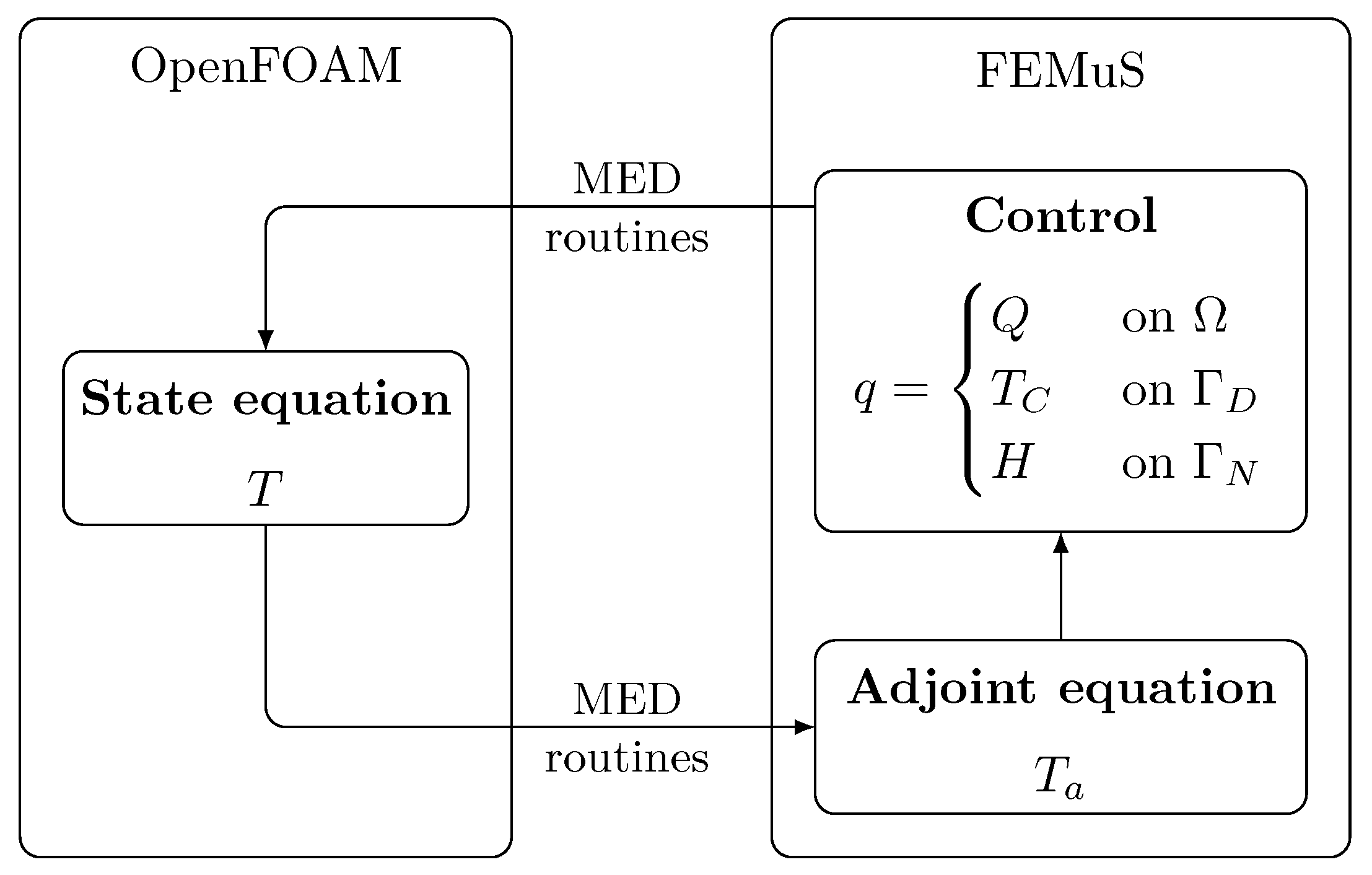
The use of optimal control theory requires the introduction of the inverse problem. The direct solution of the inverse problem, which allows rapid achievement of the goal and innovative solutions to the problem, can be carried out with the variational formulation of partial differential equations [2]. With respect to direct simulations, the resolution of an optimal control problem requires solving the optimality system formed by state, adjoint, and control coupled systems. In the context of fluid mechanics, optimal control has been already demonstrated as a valuable tool for reaching desired physical quantities and effects [3,4,5,6]. A schematic representation of a generic optimal control problem solved with the adjoint method is reported in Figure 1.
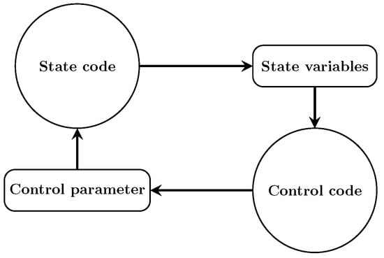
Figure 1.
Optimal control problem with adjoint equations.
For this reason, several specialized codes in solving specific physics cannot directly implement the optimality control, although using a well-validated code would greatly increase the reliability of the optimization. The solution could be to keep this standalone code for solving the specialized physics and another one for the remaining part of the optimality system. The validated code, which solves for the state system, takes data from the control equation. For that reason, the two codes must be coupled. This strategy avoids the reimplementation of well-known equations representing the state system, while different codes can be chosen to address the variational formulation arising for the adjoint and control equations.
In this paper, we present a simple temperature optimization, which is achieved by coupling our in-house FEMuS code with the widely adopted OpenFOAM code. This coupling is facilitated through the open-source MED and MEDCoupling libraries. These codes have been chosen to better address the different requirements arising from the optimal control problem. The finite element code FEMuS suits the correct variational formulation of the optimality system (particularly for the adjoint and control equations). The state equations can be solved with the widely adopted finite-volume code OpenFOAM, which has been extensively validated for most fluid mechanics applications. The coupling is performed using MED libraries and ad hoc routines added in the FEMuS and OpenFOAM codes [7,8]. A similar approach has been achieved considering the preCICE library, which offers the possibility of coupling different codes addressing multiphysics and multiscale problems. The interested reader can consult [9,10,11,12] and the references therein for further details on this alternative implementation. Regarding optimal control problems involving different physics (FSI, turbulence modeling, boundary control with fractional operators, etc.), the interested reader can consult [13,14,15] for details on the FEMuS code and [16,17] for the OpenFOAM code. Considering a similar temperature optimization problem, the interested reader can also consult [18,19] and the references therein, where a comparison of different regularization methods for the boundary control problem are presented. In [20], the author proposes a new method for solving the boundary optimal control problems of the heat equation, considering a continuous adjoint equation. In this way, they introduced a PDE describing the spatial and temporal dynamics of the boundary control variable to satisfy the regularity requirement of the adjoint variable, avoiding ill-conditioned numerical solutions.
We demonstrate the accuracy, robustness, and performance of the proposed approach with an example targeting different objectives with distributed and boundary control for each case. In the first case, the control parameter corresponds to a volumetric heat source. In the latter case, depending on whether the control is located, it may be the wall temperature (Dirichlet type) or a heat flux (Neumann type). This paper is organized as follows: First, we describe the optimal control problem with distributed or boundary controls. After that, we recall the coupling algorithm between the employed CFD codes and the MED library as a supervisor. Finally, we present the numerical results obtained with the coupled and uncoupled algorithm in order to draw some conclusions.
2. Optimal Control Problem
The finite-volume framework, of which OpenFOAM is a prime example, is traditionally well suited for flow applications of any kind. On the other hand, optimal control theory stems from the finite element framework, and its concepts are naturally evaluated in that approach. In this section, we introduce the variational formulation of the optimal control problem to better understand what components are required for the implementation of an objective-oriented framework, such as the one we display later in this paper. Each type of control is described considering the final equation system to be solved, and then the minimization algorithm is enforced using a standard conjugate gradient method.
We recall some standard notation of functional spaces [21]. Let be a domain , with , or its boundary , or a part of it. Also, let be the standard Sobolev space of order s. Naturally, we have . We now consider a cost function, or functional, in the following form:
where is a generic state variable subject to the control, is the target, u is the control parameter, and represents a penalty coefficient. With the latter parameter, the regularization term can increase or decrease the penalization by different weights on the functional. We underline that regularization terms that involve the derivative of the control variable are not considered in this paper. Naturally, the first term in (1) represents the objective term or objective functional.
The control is performed on a steady-state temperature distribution without the convective term. Therefore, considering the gradient operator ∇ and the Laplacian operator , the state equation to be satisfied by the temperature is
where represents the outward normal unit vector to the considered boundary, is the thermal diffusivity, Q the volumetric source term, and and are the two suitable functions defined on and , respectively. The boundary is split into two parts, with Neumann and Dirichlet boundary conditions applied: and . All the constraints of the problem are expressed in the Lagrangian, which is an auxiliary function defined as
where is the Lagrangian multiplier or, in this case, the adjoint temperature. Naturally, we denote by the dot product.
For each type of control, the system of equations to be solved is derived, considering the state, the adjoint, and the control equation.
2.1. Distributed Control
The distributed control parameter is a volumetric heat source Q. Therefore, the functional is written as
The Lagrange equation described in (3) can be written explicitly as
In differentiating the Lagrangian with respect to the state variable T, we obtain the system of equations for the adjoint variable
where the two boundary terms are zero due to boundary conditions on T. Then, we integrated by parts to isolate the variation
where, this time, the two boundary terms were zero, respectively, on and
thus resulting in the boundary condition terms for the adjoint variable. Rewriting (6) with the above modifications yields the adjoint problem in weak form
which must hold for every variation , and it is equivalent to the adjoint problem (9). represents the Fréchet derivative of the Lagrangian computed along the direction given by the state variable T [22].
Thus, the equation for the adjoint temperature reads
where is the Heaviside function that is equal to one only in the target region . The adjoint equation is identical to the state formulation since we only consider the Laplacian operator. The right-hand side term is different from zero only in the target regions, as indicated by the Heaviside function.
The optimal control problem can be formulated as finding the minimum of the functional (4), the condition for which the variables are considered optimal. We denote the optimal solution with an overline; thus, the optimal control must satisfy the Euler equation
Therefore, deriving the functional with respect to the control parameter Q, we obtain the Euler equation in its weak form
and thus the optimal control must satisfy the following equation
The optimal control parameter exactly follows the optimal adjoint temperature with an opposite sign and scaled by the parameter .
Although the Euler equation provides a definition of the optimal control variable, it is not sufficient for the numerical solution of the problem since it shows the behavior of the optimal solution of the optimization problem without any information on how to reach it. For most of the methods, the knowledge of the functional derivative is sufficient to calculate the direction for the functional minimization. For this reason, we define the functional derivative in the Q direction as
2.2. Neumann and Dirichlet Boundary Controls
For the Dirichlet boundary control, the control parameter is the imposed wall temperature . Therefore, the state problem becomes
where is the controlled boundary. Note that for the Dirichlet boundary case, can be interpreted as the union of and . The functional is rewritten as
where the regularization term is calculated again in . Note that, considering the temperature variable , its boundary value should be theoretically sought in the fractional space . On the other hand, since the computation of fractional operators is not straightforward, we assume to compute the regularization term considering a standard -norm. In this way, we expand the solution space for the control variable, considering less regularized solutions [23]. Similarly to the distributed control, the adjoint problem is obtained through the differentiation of the Lagrangian functional
following the same steps shown for the distributed case. Therefore, we have the system for the adjoint variable as follows:
Lastly, the Lagrangian is rewritten, integrating by part the Laplacian term, as shown in (7), and it is then differentiated with respect to the control in order to obtain the Euler equation in its weak form
and strong form
The resulting functional derivative along the direction can be defined as
For the Neumann boundary control, the control parameter is the heat flux H imposed at the wall. Therefore, the state problem and the functional are redefined as follows.
where, naturally, we now have . Therefore, the functional reads as
Again, from the Lagrangian, the control system can be derived in a manner fully analogous to the previous two cases, where the adjoint problem reads
and the optimal control expression results in
and the functional derivative along H is defined as
2.3. Conjugate Gradient Method and Numerical Solution
To numerically solve the stated problems, we employed the conjugate gradient (CG) method [24]. This minimization technique belongs to the gradient descentfamily, along with the more common steepest gradient. These techniques are used for unconstrained optimization, where the control variable q is sought in the entire control space . The CG method approximates the optimal control through a sequence such that, given a solution at the n-th step, the solution at the following step is calculated using the following formula:
where the direction is computed as
The parameter is obtained such that the directions and are conjugate with respect to the Hessian matrix , satisfying
and, where is constant, i.e., for a quadratic functional, we obtain the following expressions for
In order to make the computation easier, the formula (28) can be rewritten with the Fletcher–Reeves expression [25]
which has been implemented in our numerical algorithm.
In (29), bold symbols were used for scalar variables. Nevertheless, for the conjugate gradient method, the vectors must be interpreted as numeric vectors, i.e., the collection of the variable values on the degrees of freedom of the computational grid. Therefore, represents the numeric vector that contains this value for each node or a suitable numeric vector of values based on the specific discretization technique adopted for the system.
The numerical algorithm used for the minimization problem is a gradient algorithm. Initially, the vectors of the state variable , the adjoint variable , and the control variable were initialized along with the functional and the auxiliary variable , which represent the functional derivative at the previous iteration. The descent direction is the anti-gradient direction. The convergence theorem of the gradient algorithm can be found in [26,27,28].
After that, the time loop starts and the variables , , , and the functional are updated. Naturally, the time loop must be interpreted as an iteration loop since our system is considered to be stationary. At this point, if the convergence conditions are not satisfied, the new search direction is found calculating the current functional and the parameter . Otherwise, if the convergence is reached, the while loop is terminated, and the number of iterations and the value of the functional are collected.
Algorithm 1 illustrates only the mathematical aspects of the application since the coupling algorithm between the codes is shown in the next section. Therefore, this scheme does not take into account which code solves a specific numerical field, but it does show the logical order to find the numerical solution, thus considering the necessary steps of the minimization procedure.
| Algorithm 1 Optimal Control |
|
|
|
|
|
3. Coupling Algorithm
In this section, we will briefly recall the algorithm for code coupling employed in this work, where an optimal control problem was implemented considering two different numerical codes. The codes used in this work are FEMuS [29] and OpenFOAM [30], while the coupling interface was built to exploit the MEDCoupling library [31]. While the first two codes were used to manage CFD problems, the MEDCoupling library is a module of the SALOME platform that is developed by CEA (Commissariat à l’énergie atomique et aux énergies alternatives) and EDF (Électricité de France) to share data at the memory level, thus avoiding the use of external files. The interested reader can consult [7] and the references therein for more details on the use of the library for coupling CFD codes.
Having in mind the mathematical setting of an optimal control problem, as explained in Section 2, we will briefly recall the coupling procedure between OpenFOAM and FEMuS in the optimal control context. The main idea presented in this work is to solve the state equation for the temperature field with OpenFOAM and the adjoint equation and the control q with FEMuS. Data transfer between state and adjoint variables is achieved through a class interface based on specific MEDCoupling functions. Specifically, following the equations described in Section 2, the state equation requires the evaluation of the control parameter q solved by FEMuS. In particular, for a distributed control, q is exchanged as a volumetric source for the temperature equation in OpenFOAM, while, for the boundary control, q is transferred as a boundary condition. For the purpose of this specific paper, we added the possibility to exchange a normal gradient boundary condition from FEMus to OpenFOAM, as requested by the Neumann boundary control formulation in (20). A schematic representation of the coupling algorithm is presented in Figure 2, where and denote the Dirichlet and Neumann boundaries, respectively.
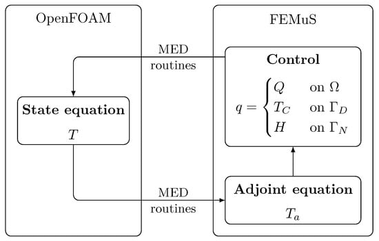
Figure 2.
Coupled algorithm diagram.
We remark that, in the coupling between a finite volume and a finite element mesh, the interpolation between the two computational grids assumes a pivotal role. Therefore, for the temperature field T solved in OpenFOAM, we exploit a interpolation toward FEMuS, where, with , we denote the polynomial of order i-th that approximates a numerical field. On the other hand, having solved q after the conjugate gradient step, we applied a interpolation from FEMuS to OpenFOAM in order to set the control q as the volumetric source/boundary condition for T.
In Algorithm 2, we report a schematic overview of the coupling algorithm between FEMuS and OpenFOAM, including the routines employed. A brief description of each routine is reported on the right. The interested reader can find details in [7].
The coupling algorithm can also be divided into two main steps. The first collects the routines useful for the initialization of the interface between the two codes. Then, we have the iteration loop with the data transfer between the two codes, including the convergence criterion. Regarding the first block, the information related to both meshes is taken into account with the routine init_interface(). In fact, a MED mesh copy for each mesh is built knowing the connectivity map and the coordinate point set (create_mesh()). After that, MED fields for all relevant variables in the exchange can be built on top of the MED meshes. Each field is populated by the source code to prepare the transfer to the target code. This step can be performed considering a cell-/node-wise initialization depending on the source field type.
The first step of the iteration loop is to solve the state variable T in OpenFOAM and then extract its values. After that, these values, centered on cells, are interpolated into the biquadratic finite element mesh of FEMuS () and then stored in the corresponding data structure of the latter code. With this information, after the functional is evaluated, a convergence check is performed. Subsequently, the FEMuS code is equipped with all the information to solve its set of equations, i.e., the adjoint variable and the control q. The finite element solutions of these numerical fields are then interpolated from biquadratic FEM elements to piecewise value () in order to transfer these data into the OpenFOAM data structure. Naturally, only the control q is transferred using the routine set_q_to_OF().
| Algorithm 2 Code Coupling |
|
|
|
|
|
4. Numerical Results
In this section, we present some numerical results that outline the mathematical framework and numerical implementation described above. Specifically, we compare an optimal temperature control problem solved with two strategies. The first approach, which serves as a benchmark case, shows the results of the uncoupled case, i.e., only the FEMuS code is employed. The second approach exploits the coupling between FEMuS and OpenFOAM through the external library MEDCoupling for data transfer, as explained in Section 3.
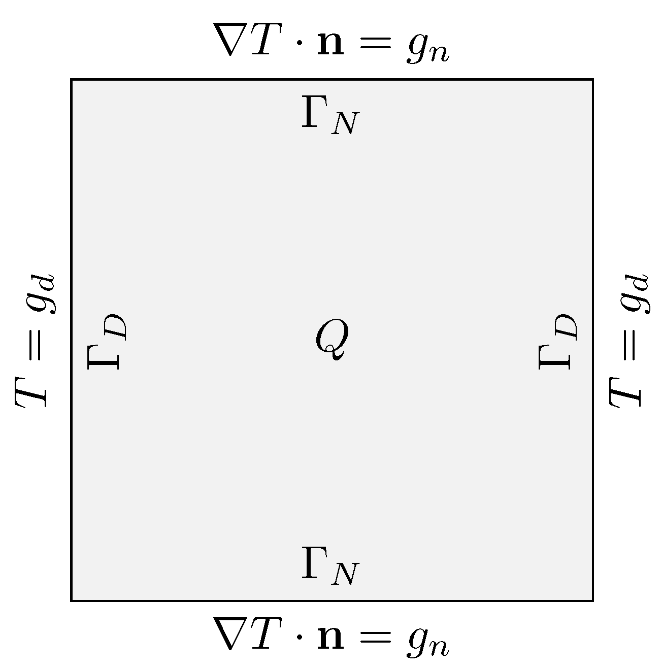
In both cases, we considered a square cavity as the problem domain, where a Poisson equation, i.e., the transport equation for the temperature field, is treated as the state equation, and and represent boundaries with Dirichlet and Neumann conditions, respectively. The problem domain with the boundary conditions is reported in Figure 3. In particular, the steady-state case with a null convective term was implemented and solved, leading to a Laplacian term equal to a right-hand side term in the form

Figure 3.
Temperature problem on the cavity.
The source field Q and the boundary conditions are described according to the different types of optimal control approach in the following sections. The boundary conditions and are considered constant in and , respectively. Boundary-type controls, which involve boundary conditions, are still initialized with or , so, at each step, we impose, at the boundary, (or ) plus (or H), where the control variable is initialized to zero.
The objective functional, which relates the state variable T with the desired temperature , remains the same for each type of control. In particular, we have
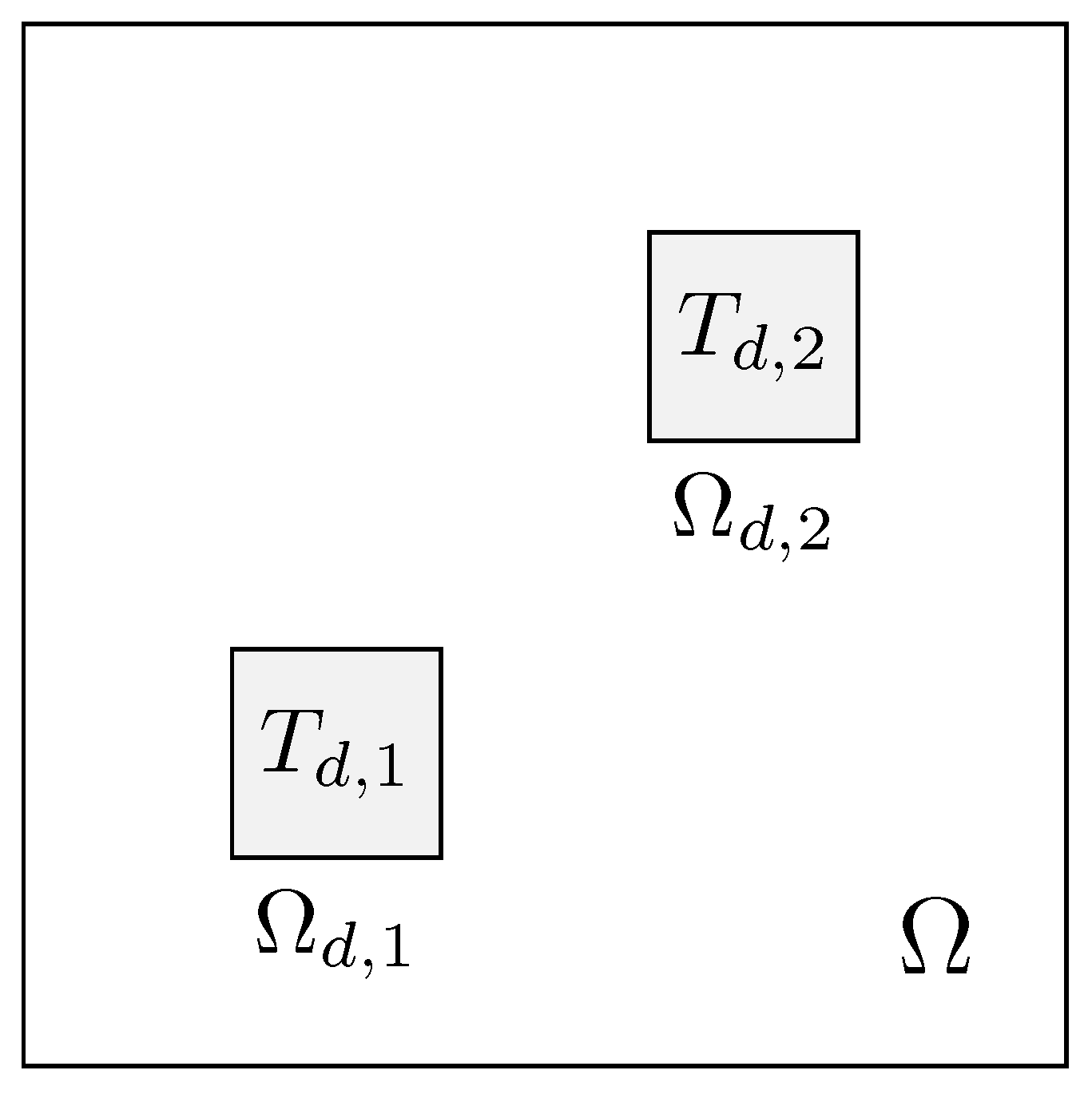
where is made up of two square subregions of the domain . In Figure 4, a schematic representation of the domain is depicted, where we have , with m. In addition, for the target regions, we have and , with targets and/or , respectively. For each simulation, we considered .

Figure 4.
Domain problem with the target regions and .
Regarding the controlled regions, for each simulation, the regularization term is assumed to be solved on . Therefore, the considered functional is
We recall that, in the case of boundary control, the second integral on the right-hand side of (32) has a meaning only on the controlled portion of the domain, which is a portion of ; thus, on the Dirichlet boundaries or on the Neumann ones.
Moreover, for each type of control, the results obtained with the coupled and uncoupled algorithms were compared. In particular, we considered the same and , and the same criterion for the convergence. Specifically, considering the average functional of 10 iterations at the iteration i, the convergence is obtained by
where is set equal to . The average functional was used instead of to avoid false exits due to the local plateaus encountered during oscillations in conjugate gradient descent.
A dimensionless formulation for the optimal control system is proposed to better show results with different dimensions or physical constants. Thus, the dimensionless state variable T, the dimensionless adjoint variable and the dimensionless control q are introduced as
where . Therefore, in our case, tends to or 1 inside the controlled regions and , respectively. Similarly, the space coordinates are adimensionalized via the square domain side L in . In order for the optimal control system to remain coherent during the transition to these dimensionless variables, the regularization factor must also be considered. Specifically, the following dimensionless transformations apply to the three types of control
In the following results, for the sake of simplicity, parameter will always be presented with its dimensional value, i.e., the value used in the simulations. However, its dimensionless value can be derived using Formula (35), with m and .
As mentioned in Section 3, one of the main issues related to the coupling of different codes is the interpolation of the numerical fields between two different computational grids. Therefore, it is important to take into account this aspect when we compare the numerical results between an uncoupled and a coupled algorithm. If we consider the temperature field obtained through the interpolation between the finite volume and the finite element grid, thus into FEMuS data structures, we should rewrite the functional in the case of the coupled algorithm. Therefore, when considering the interpolator , we have
where the control is obtained from the adjoint equation computed with the interpolated temperature, i.e.,
It is easy to understand that we have two different effects from the interpolation routine on the system of equations. The first interpolation directly acts on the functional since we compute, in the FEM grid, the distance from the target temperature considering directly the interpolated temperature. The second interpolation, which indirectly arises from the control , is evaluated considering a different equation for the adjoint variable. In fact, the effect of the interpolation can be seen on the right-hand side of (37), even if the Laplacian operator on the left-hand side acts as a smoother function; thus, the error coming from the interpolation is lower. Naturally, we should also consider the interpolation error coming from the data transfer in the opposite direction, i.e., from FEMuS to OpenFOAM.
Regarding the computational grids employed for the coupling algorithm, we set it to have the same number of degrees of freedom between the two codes. For this reason, to clarify the notation when the size of a grid is built with even numbers, e.g., , we refer to the finite element grid, where these numbers represent the elements’ number . As a result, the corresponding FV grid size is represented by odd numbers, such as . Indeed, we recall that, considering biquadratic elements for finite element grids, its degrees of freedom are equal to when considering a square domain with a structured quadrilateral mesh.
4.1. Distributed Control
In this section, we report the numerical results related to the distributed control, with both numerical methods, i.e., the coupled and uncoupled algorithm. We recall that, for the distributed case, the control q acts as the volumetric source on the right-hand side of the temperature equation, i.e., Q. Regarding the boundary conditions, we obtained homogeneous Dirichlet and Neumann boundary conditions on and , respectively.
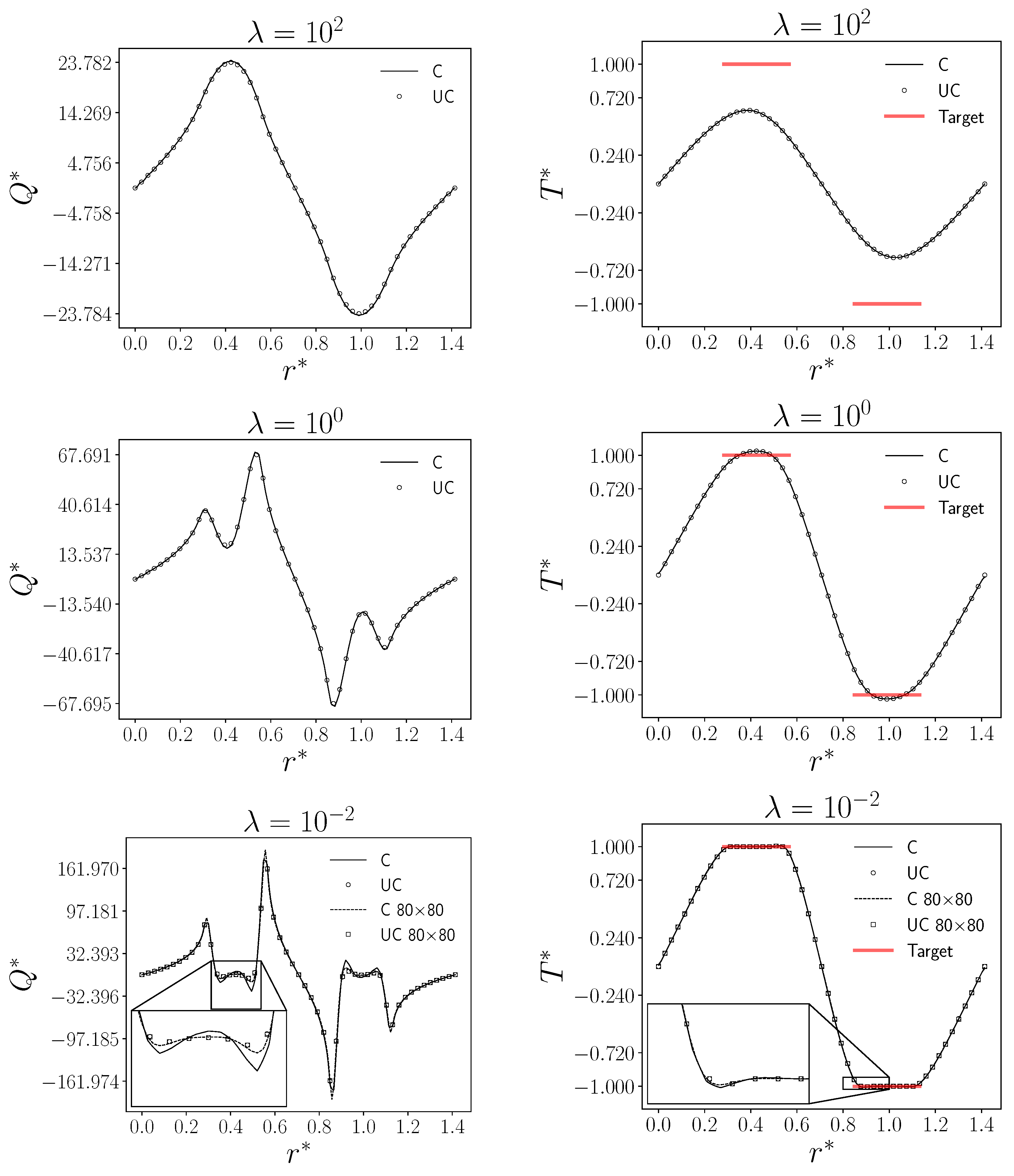
In Figure 5, the control and the non-dimensional state variable are reported, considering different values of the parameter from to . In particular, we show the variables as a function of the dimensionless length , which corresponds to the diagonal of the domain (from the lower left corner to the upper right corner), with a value ranging from 0 to . The coordinate allows us to evaluate the state and the control variable in both controlled regions. In the following, we denote, by UC, the uncoupled results (circular marker), while, with the label C, we denote the coupled code results with a solid line. The target value is shown with a solid red line.
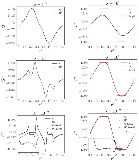
Figure 5.
From (top) to (bottom), control Q (left) and temperature (right) for different , as a function of the non-dimensional diagonal for a grid. On the bottom, the case with a grid is also reported.
In Figure 5, we show the different behavior of the control parameter Q with different values of and the corresponding effect on the state variable in the controlled regions. As decreases, the control becomes less smooth and produces a sharp behavior near the controlled regions, as expected. In fact, the case with represents the less regularized solution, with corresponding temperatures in the controlled region very close to the target value. Otherwise, with a , the control has a low effect on the state variable, which cannot reach the target value in the controlled regions.
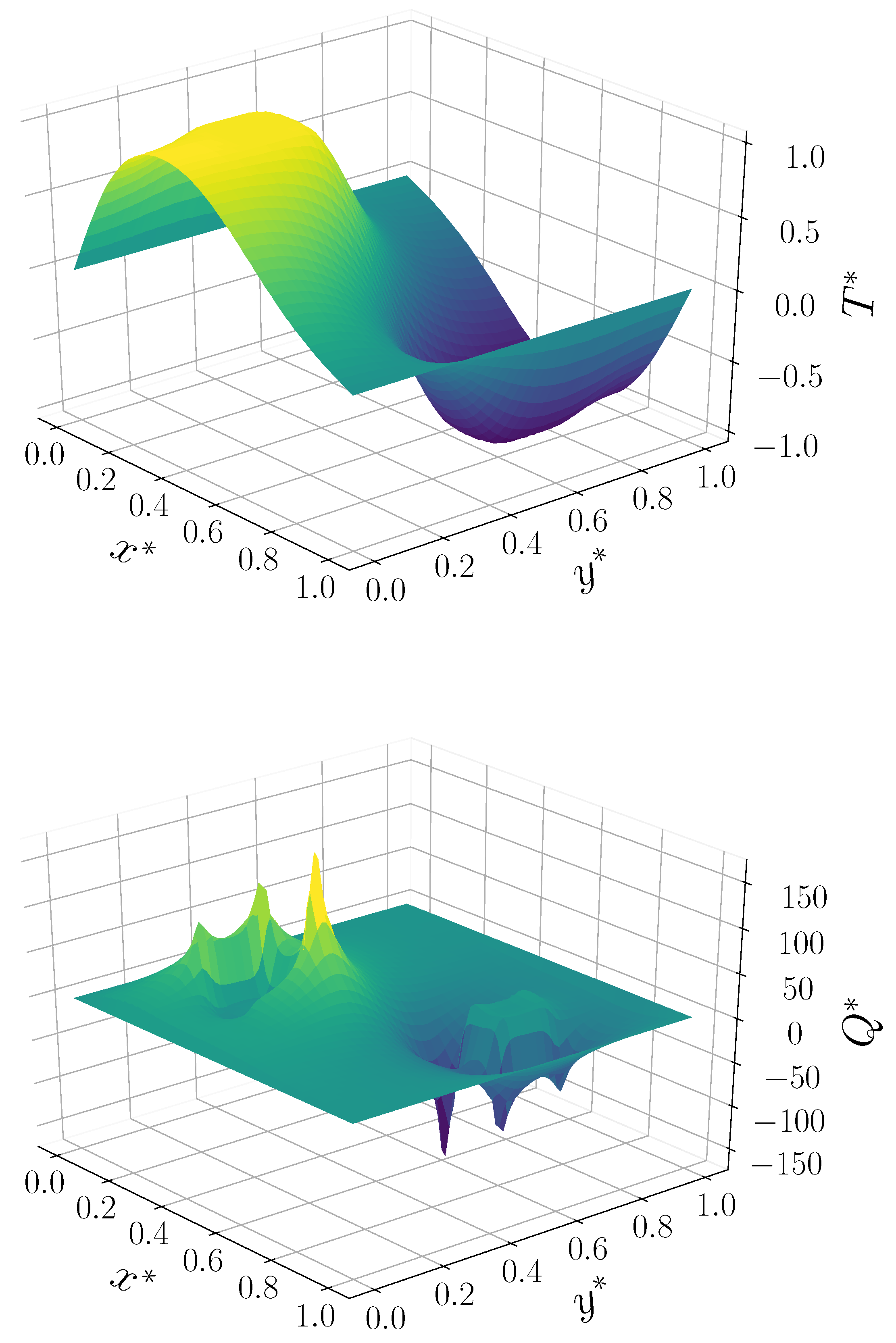
In Figure 6, a surface plot of the non-dimensional temperature and the non-dimensional control over the whole domain is reported. Specifically, we display only the case with the lowest , considering a finite element grid. The symmetric behavior of these variables is shown. Moreover, a sharp trend of was present near the target regions, where several peaks can be observed. Regarding the temperature field, as expected, two plateaus were present in the target regions, with opposite values close to 1 and .

Figure 6.
Dimensionless temperature (top) and control (bottom).
Table 1 reports the functional value and the number of iterations for the three different cases previously presented. The table lets us better understand the numerical results depicted in Figure 5. Indeed, for different cases, the first column represents the minimum of the functional, while the second column reports the number of iterations needed to reach the convergence condition. The first row reports the results for the coupled case, while the second row represents the uncoupled scenario. We recall that these results refer to a computational FEM grid with elements and a corresponding grid for the FVM to have the same number of degrees of freedom. Regarding , with larger values, we obtain a good match for both algorithms, while a larger difference can be noted for the lowest value of .

Table 1.
Minimum of the functional and number of iterations for the different cases of the distributed control with both algorithms. In the last column, for the lowest value, the results for the refined grid are also reported.
For , we observed some discrepancies between the coupled and uncoupled results. This phenomenon can be explained by considering the errors introduced during field interpolation and data transferred from one code to the other. As the optimal state is approaching, the distance of the state from the desired temperature decreases, making the interpolation error on T at first negligible and then increasingly important. This interpolation error limits the achievement of the real optimum state since we are not able to obtain a sufficiently accurate control.
The interpolation error can be improved by increasing the number of degrees of freedom. In fact, as shown in Figure 5 on the right, we also reported the same case of obtained with a refined grid, with a dashed line for the coupled case and with square markers for the uncoupled one. For the uncoupled case, small differences can be noticed because the simulation has already found its optimum, but, in the coupled approach, improvements can be obtained to stir Q very close to the uncoupled results. These conclusions can be drawn from Table 1, where the distance between the two minima decreases considering the refined solution. In addition, the relative errors between the functional minimum increased by decreasing the value of , going from 1 to . However, the latter value corresponding to the lowest can be improved until around with a refined grid.
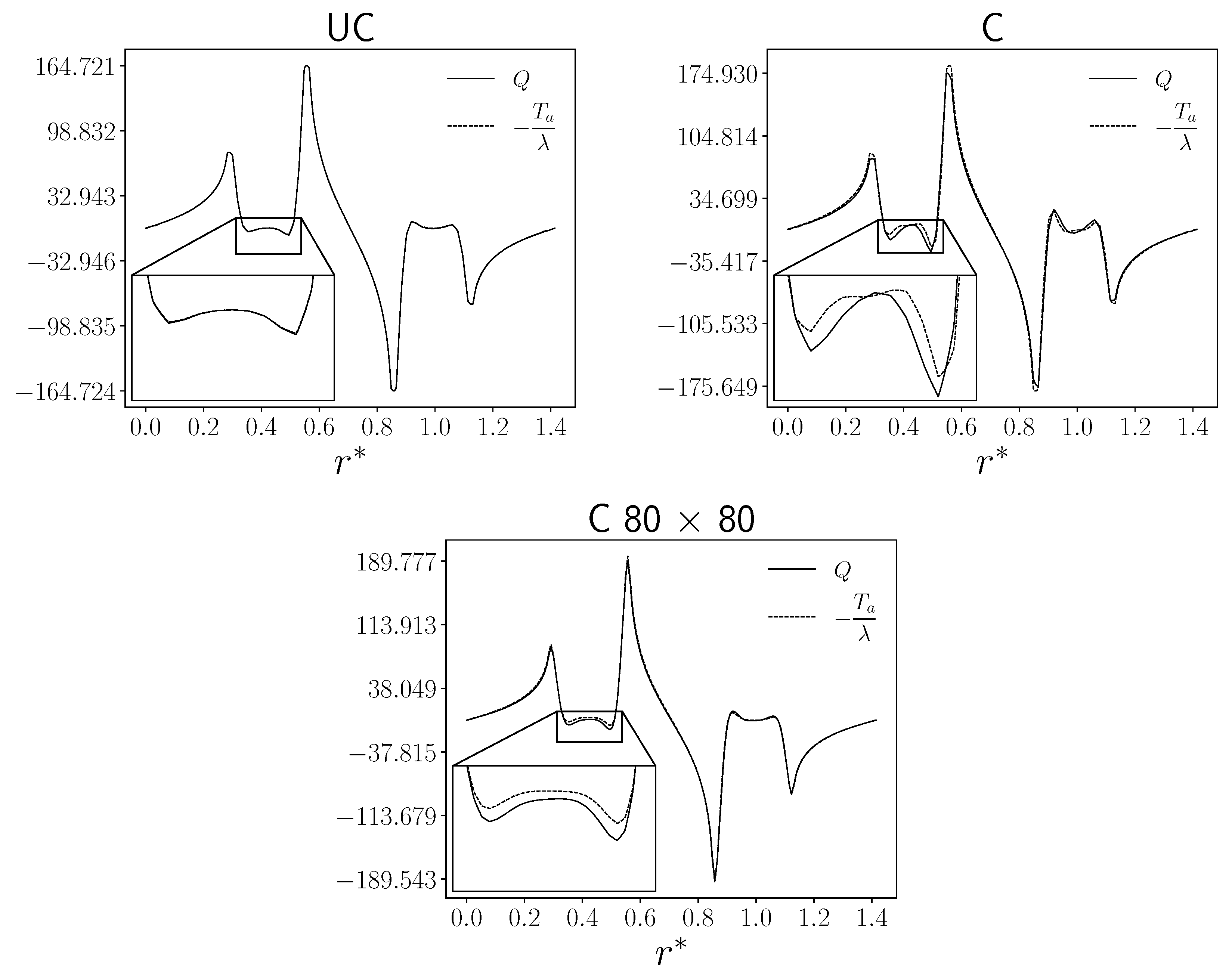
A measure of the quality of the optimization convergence can be obtained using the Euler expression defined in (11). We recall that uncoupled algorithms must be used when state and adjoint equations are solved with different solvers. As shown in Figure 7, we compared the obtained control Q with its analytic optimal expression . We can notice that, for the uncoupled approach, there is a perfect agreement between the two lines, while some differences are present for the coupled case. As said before, we obtained better results considering the refined coupled approach at the bottom. Comparing the two approaches, we recall the previous considerations about the functional minimum. We can, therefore, assume the accuracy of the uncoupled simulation, which we use as a reference case.
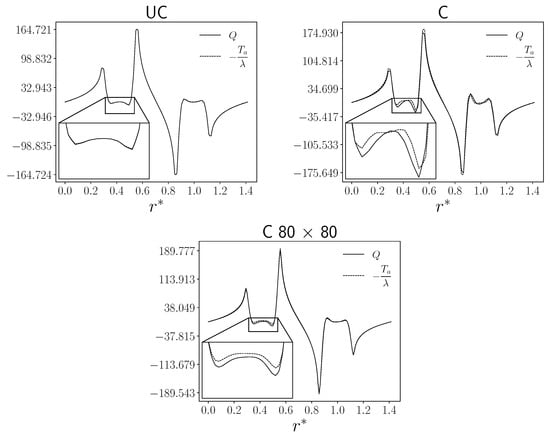
Figure 7.
Optimal control Q and its analytic expression at the optimum state. Uncoupled case at the (top left), coupled case at the (top right), and the refined coupled case on the (bottom).
The number of iterations was different between the two algorithms. Actually, this is true considering the first two values of where the coupled case needs more iterations to satisfy the convergence condition. For example, considering , we saw an increase of almost one order of magnitude for the coupled case. However, this difference decreased when decreased sincem for the most controlled case, i.e., , the number of iterations was similar. In the last column, we report, for the lowest , the results for a refined case. Refining the grid, we noticed that we reached a lower functional value while the number of iterations increased.
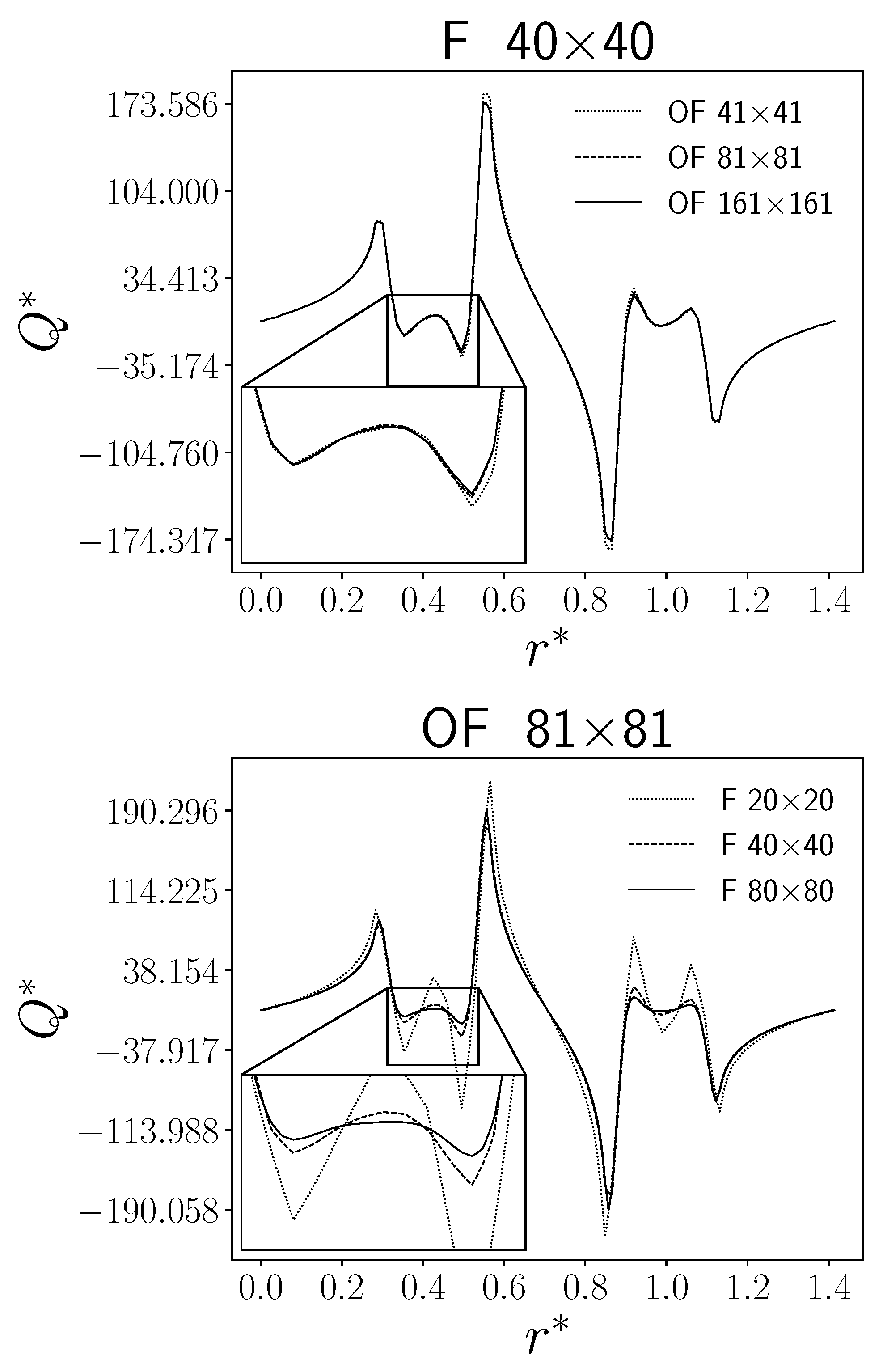
For the distributed case, we also investigated the influence of the difference between the degrees of freedom of the two meshes. This comparison aimeed to evaluate the impact of the MED-interpolating function on the overall behavior of the algorithm, especially for the shape of the control . Therefore, we considered three different grids of the FVM code (OpenFOAM) by fixing the FEM computational grid with the same degree of freedom as the intermediate FVM grid. On the other hand, the same simulations were performed considering a fixed FVM grid and varying the FEM one. The results rea reported in Figure 8, where F denotes the FEMuS grid and OF the OpenFOAM grid. For these results, we only considered the case with , and the control is reported as a function of the dimensionless diagonal coordinate .

Figure 8.
Control Q for the different combinations of degrees of freedom between the two codes as a function of . The FEM grid (F) and the FVM grid (OF) are fixed on the (top) and (bottom), respectively.
From Figure 8, one can see the difference in the control as a function of the computational grids. The finite volume grid change, as shown on the top, did not seem to influence the solution of the equation systems. On the bottom, the situation was different when considering the coarsest FEM grid since, for finer grids, the results were comparable with the picture on the top. At least for this application, the OpenFOAM grid had much less influence than the FEMuS grid on the shape of the control. The interpolation error occurs when the projected field no longer provides a good approximation of the original one, i.e., when the target grid resolution is not fine enough. This shows that the error occurs when the temperature field is projected from the grid to the of the FEMuS grid since the interpolation control is not sufficiently detailed.
As shown in Table 2, we can confirm the effectiveness of grid refinement in the two codes: we had a much greater impact on the minimum of the functional by varying the FEMuS mesh compared to varying the OpenFOAM mesh. Moreover, it is interesting to note that the minimum number of iterations corresponds to the case where the two meshes had the same degrees of freedom.
Table 2.
The minimum of the functional and the number of iterations for the case when varying the grid ratio of the two codes. In the top row, the FEMuS mesh is kept fixed with 40 × 40 resolution and the OpenFOAM mesh is varied. In the bottom row, the opposite situation is reported using OpenFOAM at 81 × 81 resolution.
4.2. Boundary Control
In this section, we report the boundary control cases for two types of boundary conditions: Dirichlet and Neumann. The volumetric source of the state equation was equal to zero, leading to a Poisson equation for T. The boundary conditions separately correspond to the control q for the Dirichlet and the Neumann case, where the uncontrolled pair of boundaries stay homogeneous.
4.2.1. Dirichlet Boundary Control
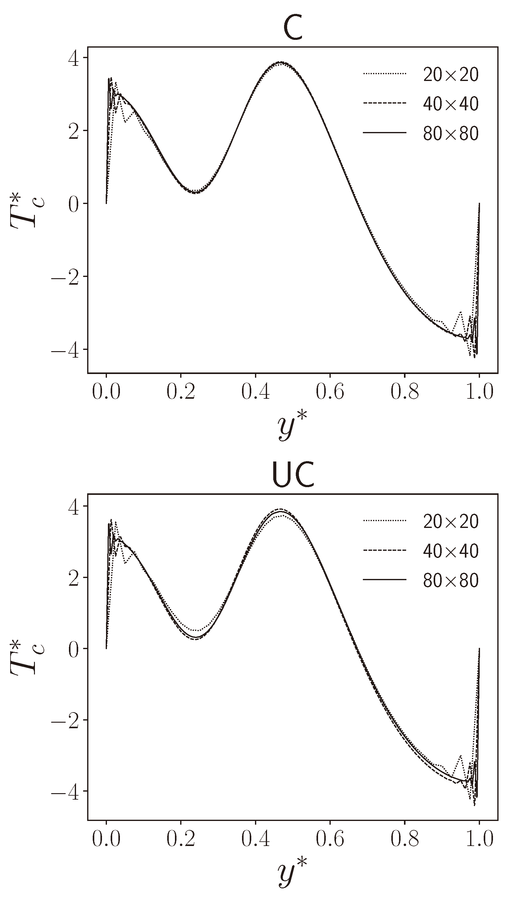
For the Dirichlet boundary control, we also performed a standard grid convergence test to verify the goodness of the numerical results. As shown in Figure 9, on the left, the state variable in the controlled domain, that is, the control parameter q (), which is imposed as a boundary condition, is reported. Since the simulation was symmetric with respect to the y axes, we reported only one boundary.
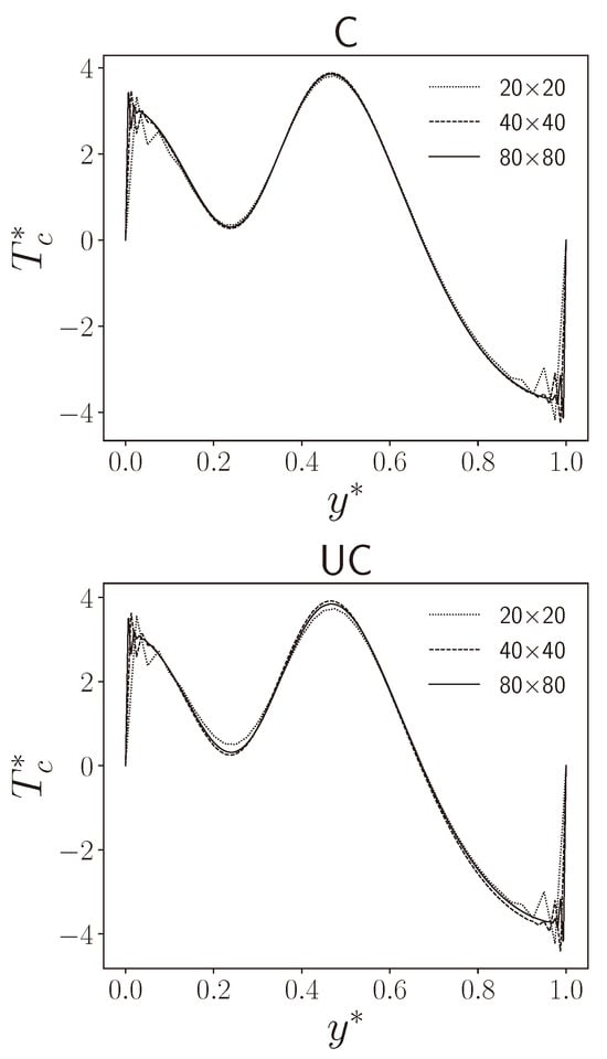
Figure 9.
Grid convergence for the Dirichlet boundary control for for the coupled (top) and uncoupled (bottom) cases. Non-dimensional temperature on the left controlled boundary for three different grid sizes.
A convergence comparison between the coupled and uncoupled cases is shown in Figure 9. Good grid convergence can be seen for both algorithms, confirming the reliability of the numerical approach. In fact, the finest grid presents a solution that tends to be smooth near the boundary of the control region. The boundary of , near the corner nodes of the domain, had a singular point.
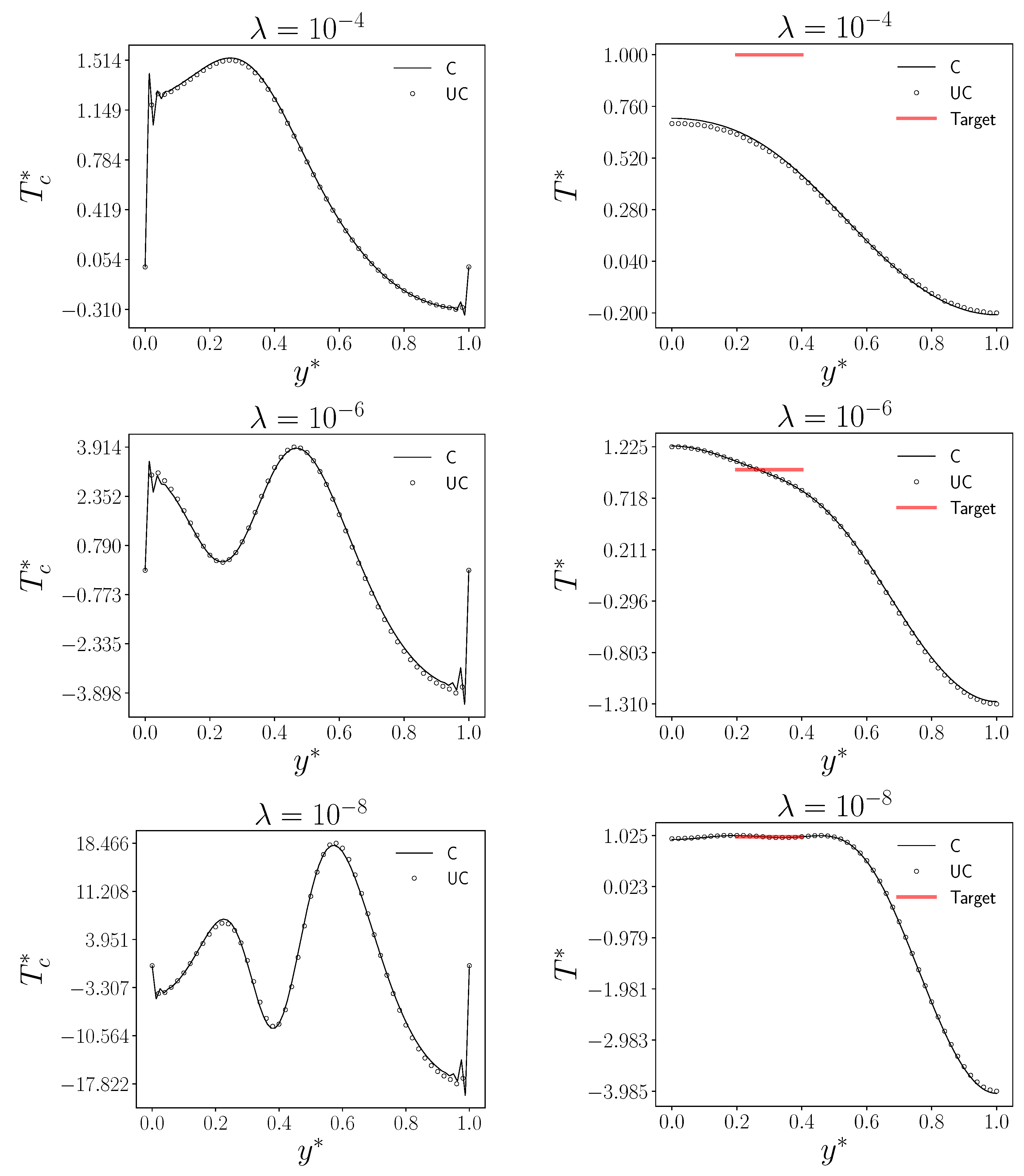
As shown in Figure 10, the control and the state variable were reported for the Dirichlet boundary control for three values of equal to , and . The notation adopted in the graphs is the same as the distributed case. Since the results were symmetric to the line , the control was reported only for the left boundary. For the state variable, a plot was made considering the match with the target region .
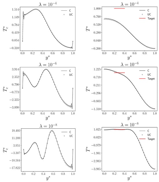
Figure 10.
From (top) to (bottom), control (left) and temperature (right) for different , and as a function of the non-dimensional coordinate , respectively, on the left wall for the control (at ) and in the middle of the target region 1 for the state variable () on a grid.
We drew similar conclusions to those in the distributed case. Specifically, a good match with the temperature target value can be obtained with a low value of , corresponding to the less regular trend of the control . For this case, we had a flat behavior of very close to 1, i.e., the red line, in correspondence with the controlled region . The distance with the target region was higher considering the case with , while, with , the temperature can only intersect without reproducing its constant value in the entire region.
As shown in Table 3, the functional minimum and the number of iterations are reported for the Dirichlet boundary control. We can observe a better behavior of the coupled code with respect to the uncoupled case on both the minimum reached and the number of iterations. In any case, the differences between the two cases were minimal.
Table 3.
The minimum functional and number of iterations for the different cases of the Dirichlet boundary control with both algorithms for a grid.
4.2.2. Neumann Boundary Control
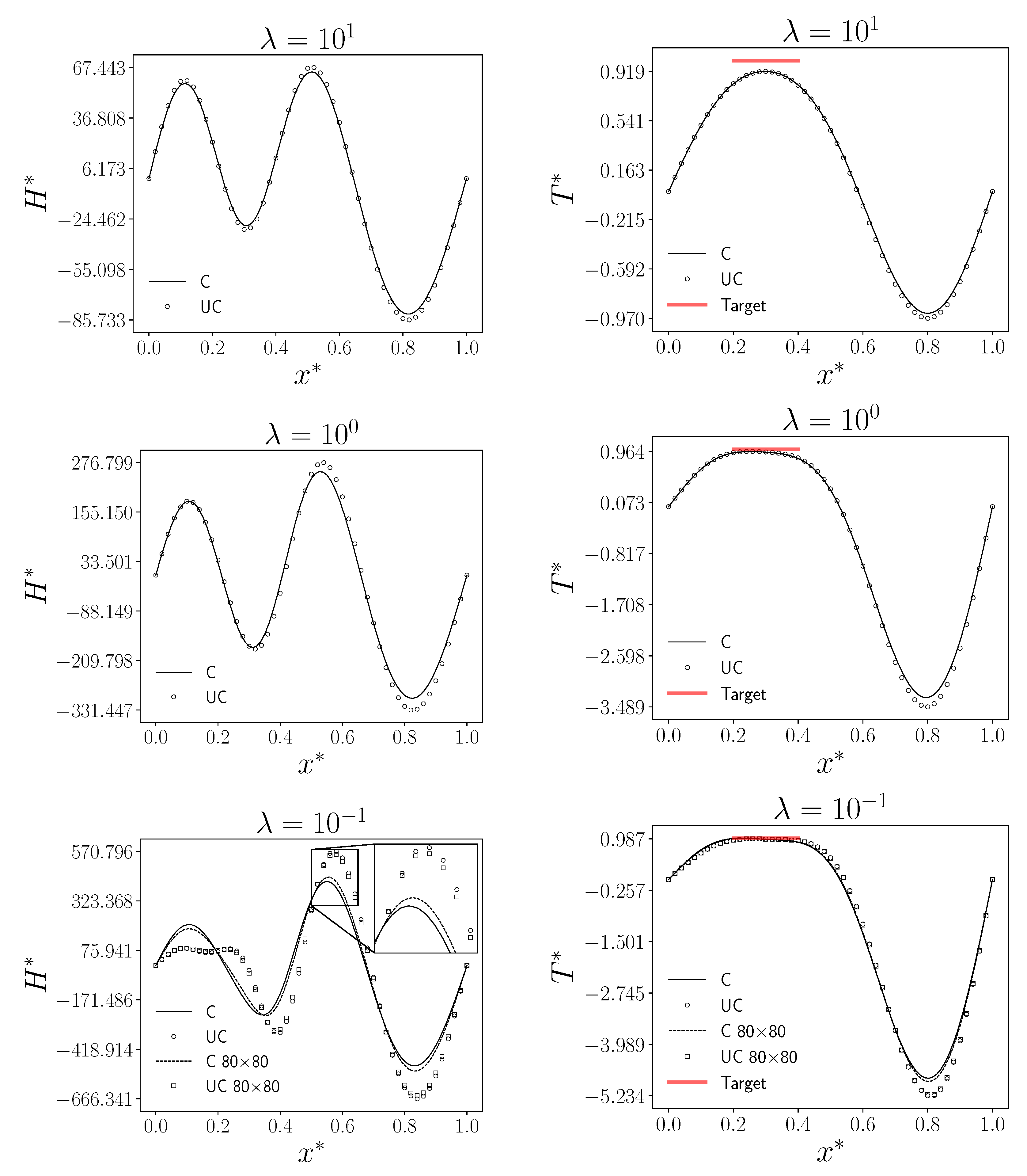
We present now the numerical results obtained with the Neumann boundary control, following (23). In this case, three values of were used to test the influence of the control H on the state equation. As shown in Figure 11, the numerical results for the Neumann boundary control are reported with the considered . Due to symmetry, we report only one of the two boundaries (the bottom one) for the control H.

Figure 11.
From (top) to (bottom), control (left) and temperature (right) for different , and as a function of the non-dimensional coordinate , respectively, on the lower wall for (at ) and in the middle of the target region 1 for () on a grid. For the case , the results for a grid are also reported.
The similar comments of the previous cases are also true for the Neumann boundary control. A good agreement between the state variable and the target temperature can be obtained only with small values of since, for higher values of this parameter, the control does not sufficiently influence the temperature . This consideration is graphically represented in Figure 11, where the variables are plotted as a function of the distance between the red line and the solutions for . For low values of , the major difference is present near the target region, whereas, for the uncoupled control, seems to be more flat with respect to the coupled result. Once again, we reported the same case of obtained with a refined grid, with a dashed line for the coupled case and square markers for the uncoupled one. Similarly, as in the distributed case, we can observe that the coupled and uncoupled results became similar as the grid became finer. On the other hand, these differences did not influence the state temperature , which is in perfect agreement with the desired value for both algorithms. Small differences can be noticed for (far from the target region), where the uncoupled algorithm reached a lower value.
As shown in Table 4, the functional minimum value and the number of iterations for both algorithms are reported. For the lower case of , which is the last column on the right, the results on a refined grid were also investigated. In this case, the number of iterations increased both in the coupled and in the uncoupled codes, decreasing the value of . For high values of , the functional minimum is similar in both algorithms, while the coupled case presents a higher number of iterations. A slightly different can be seen for the lowest value of . The case with shows the same pattern as the distributed case above. For the finer grids on the coupled code, we obtained a lower minimum of the functional with a higher number of iterations, while, in the uncoupled case, the number of iterations decreased. With refined meshes, the difference between the values of the functional minimum decreased, confirming the improvement of the results when considering finer computational grids. This similarity can be justified considering the fact that both the distributed and Neumann cases shared the same control expression based on the adjoint temperature. In fact, this behavior was not present in the Dirichlet control since the gradient of the adjoint temperature was used as the control parameter.
Table 4.
The minimum of the functional and number of iterations for the different cases of the Neumann boundary control with both algorithms for a grid. In the last column, for the lowest value, the results for the refined grid are also reported.
5. Conclusions
In this work, an optimal control problem has been presented considering the steady-state heat equation with a vanishing convective term. Specifically, the minimization problem was solved with the adjoint equation, while the control parameter was handled with a standard conjugate gradient technique.
Moreover, we compared the simulation results by also considering a numerical code coupling between the finite element FEMuS code and the finite volume code OpenFOAM. In particular, while the state equation was solved in OpenFOAM, the adjoint and the control were solved in FEMuS. The data transfer was managed by the external library MEDCoupling, which was able to take the state variable T from OpenFOAM for the FEMuS adjoint equation. The inverse path was followed by the control variable Q, and it was obtained from FEMuS and transferred to OpenFOAM as the RHS (distributed control) or as a boundary condition (boundary control).
The numerical results obtained with the coupling framework are compared with the ones resulting from the standalone FEMuS solution. For the three types of control problems, a good agreement between the numerical solutions of the two algorithms was obtained. Regarding the interpolation error, some differences can be seen considering low values of since, for these cases, the result of the grid interpolation of T affects the control q, which is very sharp.
Extension to other systems of equations, from Navier–Stokes to turbulence modeling, will be studied in future work, with the purpose of searching boundary data that optimize the multiphysics problems already validated in open-source codes such as OpenFOAM.
Author Contributions
Conceptualization, S.B., G.B., A.C., F.G., S.M. and L.S.; Methodology, S.B., G.B., A.C., F.G., S.M. and L.S.; Writing—original draft, S.B., G.B., A.C., F.G., S.M. and L.S.; Writing—review and editing, S.B., G.B., A.C., F.G., S.M. and L.S. All authors have read and agreed to the published version of the manuscript.
Funding
This research received no external funding.
Data Availability Statement
The raw data supporting the conclusions of this article will be made available by the authors on request.
Conflicts of Interest
The authors declare no conflicts of interest.
References
- Manzoni, A.; Quarteroni, A.; Salsa, S. Optimal Control of Partial Differential Equations; Springer: Berlin/Heidelberg, Germany, 2021. [Google Scholar]
- Gunzburger, M.D. Perspectives in Flow Control and Optimization; SIAM: Philadelphia, PA, USA, 2002. [Google Scholar]
- Abergel, F.; Casas, E. Some optimal control problems of multistate equations appearing in fluid mechanics. ESAIM Math. Model. Numer. Anal. 1993, 27, 223–247. [Google Scholar] [CrossRef]
- Sritharan, S.S. Optimal Control of Viscous Flow; SIAM: Philadelphia, PA, USA, 1998. [Google Scholar]
- Abergel, F.; Temam, R. On some control problems in fluid mechanics. Theor. Comput. Fluid Dyn. 1990, 1, 303–325. [Google Scholar] [CrossRef]
- Aulisa, E.; Cervone, A.; Manservisi, S.; Seshaiyer, P. A multilevel domain decomposition approach for studying coupled flow applications. Commun. Comput. Phys. 2009, 6, 319–341. [Google Scholar] [CrossRef]
- Barbi, G.; Cervone, A.; Giangolini, F.; Manservisi, S.; Sirotti, L. Numerical Coupling between a FEM Code and the FVM Code OpenFOAM Using the MED Library. Appl. Sci. 2024, 14, 3744. [Google Scholar] [CrossRef]
- Da Vià, R. Development of a Computational Platform for the Simulation of Low Prandtl Number Turbulent Flows. Ph.D. Thesis, University of Bologna, Bologna, Italy, 2019. [Google Scholar]
- Bungartz, H.J.; Lindner, F.; Gatzhammer, B.; Mehl, M.; Scheufele, K.; Shukaev, A.; Uekermann, B. preCICE—A fully parallel library for multi-physics surface coupling. Comput. Fluids 2016, 141, 250–258. [Google Scholar] [CrossRef]
- Chourdakis, G.; Davis, K.; Rodenberg, B.; Schulte, M.; Simonis, F.; Uekermann, B.; Abrams, G.; Bungartz, H.J.; Yau, L.C.; Desai, I.; et al. preCICE v2: A sustainable and user-friendly coupling library. Open Res. Eur. 2022, 2, 51. [Google Scholar] [CrossRef] [PubMed]
- Kim, D.; Kim, J. Simulation of a conjugate heat transfer using a preCICE coupling library. In Proceedings of the Transactions of the Korean Nuclear Society Virtual Spring Meeting, Jeju-si, Republic of Korea, 9–10 July 2020; pp. 9–10. [Google Scholar]
- Martin, P.; Rosier, L.; Rouchon, P. On the reachable states for the boundary control of the heat equation. Appl. Math. Res. Express 2016, 2016, 181–216. [Google Scholar] [CrossRef]
- Chirco, L. On the Optimal Control of Steady Fluid Structure Interaction Systems. Ph.D. Thesis, University of Bologna, Bologna, Italy, 2020. [Google Scholar]
- Giovacchini, V. Development of a Numerical Platform for the Modeling and Optimal Control of Liquid Metal Flows. Ph.D. Thesis, University of Bologna, Bologna, Italy, 2022. [Google Scholar]
- Chierici, A. Mathematical and Numerical Models for Boundary Optimal Control Problems Applied to Fluid-Structure Interaction. Ph.D. Thesis, University of Bologna, Bologna, Italy, 2021. [Google Scholar]
- Othmer, C. A continuous adjoint formulation for the computation of topological and surface sensitivities of ducted flows. Int. J. Numer. Methods Fluids 2008, 58, 861–877. [Google Scholar] [CrossRef]
- Önder, A.; Meyers, J. Optimal control of a transitional jet using a continuous adjoint method. Comput. Fluids 2016, 126, 12–24. [Google Scholar] [CrossRef]
- Bornia, G.; Chierici, A.; Ratnavale, S. A comparison of regularization methods for boundary optimal control problems. Int. J. Numer. Anal. Model. 2022, 19, 329–346. [Google Scholar]
- Carthel, C.; Glowinski, R.; Lions, J.L. On exact and approximate boundary controllabilities for the heat equation: A numerical approach. J. Optim. Theory Appl. 1994, 82, 429–484. [Google Scholar] [CrossRef]
- Park, H.; Lee, W. A new numerical method for the boundary optimal control problems of the heat conduction equation. Int. J. Numer. Methods Eng. 2002, 53, 1593–1613. [Google Scholar] [CrossRef]
- Adams, R.A.; Fournier, J.J. Sobolev Spaces; Elsevier: Amsterdam, The Netherlands, 2003. [Google Scholar]
- Tröltzsch, F. Optimal Control of Partial Differential Equations: Theory, Methods, and Applications; American Mathematical Soc.: Washington, DC, USA, 2010; Volume 112. [Google Scholar]
- Chierici, A.; Giovacchini, V.; Manservisi, S. Analysis and Computations of Optimal Control Problems for Boussinesq Equations. Fluids 2022, 7, 203. [Google Scholar] [CrossRef]
- Nazareth, J.L. Conjugate gradient method. Wiley Interdiscip. Rev. Comput. Stat. 2009, 1, 348–353. [Google Scholar] [CrossRef]
- Fletcher, R.; Reeves, C.M. Function minimization by conjugate gradients. Comput. J. 1964, 7, 149–154. [Google Scholar] [CrossRef]
- Ciarlet, P.G.; Miara, B.; Thomas, J.M. Introduction to Numerical Linear Algebra and Optimisation; Cambridge University Press: Cambridge, UK, 1989. [Google Scholar]
- Gruver, W.A.; Sachs, E. Algorithmic Methods in Optimal Control; Pitman Publishing: Lanham, MD, USA, 1981. [Google Scholar]
- Gunzburger, M.D.; Manservisi, S. The velocity tracking problem for Navier–Stokes flows with bounded distributed controls. SIAM J. Control Optim. 1999, 37, 1913–1945. [Google Scholar] [CrossRef]
- Barbi, G.; Bornia, G.; Cerroni, D.; Cervone, A.; Chierici, A.; Chirco, L.; Viá, R.; Giovacchini, V.; Manservisi, S.; Scardovelli, R.; et al. FEMuS-Platform: A numerical platform for multiscale and multiphysics code coupling. In Proceedings of the 9th International Conference on Computational Methods for Coupled Problems in Science and Engineering, Coupled Problems 2021, Sardinia, Italy, 13–16 June 2021; pp. 1–12. [Google Scholar]
- Jasak, H. OpenFOAM: Open source CFD in research and industry. Int. J. Nav. Archit. Ocean Eng. 2009, 1, 89–94. [Google Scholar]
- Ribes, A.; Caremoli, C. Salome platform component model for numerical simulation. In Proceedings of the 31st Annual International Computer Software and Applications Conference (COMPSAC 2007), Beijing, China, 24–27 July 2007; Volume 2, pp. 553–564. [Google Scholar]

Disclaimer/Publisher’s Note: The statements, opinions and data contained in all publications are solely those of the individual author(s) and contributor(s) and not of MDPI and/or the editor(s). MDPI and/or the editor(s) disclaim responsibility for any injury to people or property resulting from any ideas, methods, instructions or products referred to in the content. |
© 2025 by the authors. Licensee MDPI, Basel, Switzerland. This article is an open access article distributed under the terms and conditions of the Creative Commons Attribution (CC BY) license (https://creativecommons.org/licenses/by/4.0/).