Abstract
The Ueda oscillator is one of the most popular and studied nonlinear oscillators. Whenever subjected to external periodic excitation, it exhibits a fascinating array of nonlinear behaviors, including chaos. This research introduces a novel fractional discrete Ueda system based on -th Caputo fractional difference and thoroughly investigates its chaotic dynamics via commensurate and incommensurate orders. Applying numerical methods like maximum Lyapunov exponent spectra, bifurcation plots, and phase plane. We demonstrate the emergence of chaotic attractors influenced by fractional orders and system parameters. Advanced complexity measures, including approximation entropy () and complexity, are applied to validate and measure the nonlinear and chaotic nature of the system; the results indicate a high level of complexity. Furthermore, we propose a control scheme to stabilize and synchronize the introduced Ueda map, ensuring the convergence of trajectories to desired states. MATLAB R2024a simulations are employed to confirm the theoretical findings, highlighting the robustness of our results and paving the way for future works.
MSC:
39A33; 39A12; 39A28
1. Introduction
Oscillations refer to repetitive rotational or oscillatory motion around a mean position. These motions can arise from various factors, such as gravitational forces, external forces acting on moving objects, or natural phenomena like moving air or electromagnetic waves. The types of oscillations observed in nature and engineering systems are highly diverse, encompassing mechanical oscillations, electromagnetic waves, acoustic vibrations, and more [1]. In 1980, Japanese researcher Ueda conducted detailed studies on a specific type of non-linear oscillation, significantly contributing to understanding chaotic dynamics. His work included the study of the Duffing oscillator, a well-known non-linear forced oscillator. In addition, Ueda explored several hybrid chaotic forced oscillators based on the Duffing system, including the Duffing-Van der Pol oscillator and the Rayleigh-Duffing oscillator. He also examined the Ueda oscillator and Single Degree of Freedom (Sdof) oscillator, broadening the scope of chaotic and non-linear oscillatory systems [2]. These oscillatory models represent systems where the damping variable, restoring force, and varying parameters interact in non-linear ways. The models provide valuable frameworks for understanding the behavior of non-linear systems and the complex effects that can arise within them. Such studies are essential for representing oscillations in dynamic systems and analyzing the intricate behaviors that emerge from their interactions [3].
Understanding chaos in oscillatory systems is a comprehensive study of the interactions and changes that occur over time [4]. Chaos phenomena analysis may be important for examining a system’s behavior and identifying the factors that affect it. Chaos in oscillatory systems can be caused by multiple interactions between variables or deviation from expected behavior due to noise or disturbances in the system [5]. Furthermore, the randomness, unpredictability, and sensitivity to initial conditions of chaotic systems facilitate the generation of pseudo-random sequences and enhanced data encryption. The inherent advantages of chaotic behaviors have resulted in significant progress across various fields, including data encryption, secure communications, image and signal processing, and optimization techniques [6,7,8]. For instance, in reference [6] investigates an innovative, secure image transmission method utilizing the synchronization hyperchaotic maps, while Jain et al. [7] research on medical data encryption utilizing a multiple chaotic discrete model, whereas in [8], discrete transform domain encryption and image encryption implementation have been studied. The Ueda oscillation can be an interesting topic in physics, engineering, and mathematics due to its complex dynamical properties, including unusual behavior transitions and frequency and position changes. For instance, researchers are very curious about its practical applications. They are used in robotics control, digital signal processing, modeling biological interactions, and much more [9]. Discrete oscillatory maps have not attracted as much attention as continuous oscillatory systems, which have been extensively researched. Typically, extensive research has been conducted on continuous-time oscillator systems, whereas discrete-time oscillator systems have received comparatively limited attention and discourse. Additionally, chaotic maps encompass numerous complex dynamic phenomena, such as multi-stability, coexisting bifurcations, coexisting attractors, and hidden attractors [10,11].
Recently, fractional calculus has provided significant advantages across a wide range of fields, offering powerful tools for researchers and scientists to analyze and understand complex systems with greater depth and accuracy compared to traditional integer-order derivatives. By incorporating fractional-order derivatives, researchers can capture a higher level of chaotic behavior and subtle dynamic properties often missed with standard approaches [12]. Fractional calculus enhances the modeling of various phenomena, including memory effects and hereditary properties intrinsic to many physical and biological systems. Mainly, integer-order systems have been the focus of previous research on fractional oscillators. However, limited research has been undertaken to examine the behavior and characteristics of discrete fractional oscillators with integer order. Moreover, discrete chaotic models are characterized by irregular oscillations, bifurcations, and complex patterns in their state-space trajectories. Despite their seemingly random behavior, discrete chaotic systems follow deterministic rules governed by mathematical equations. In practice, discrete fractional chaotic oscillator systems have the advantage of not having the parameter sensitivity issues that fractional continuous systems do. Therefore, researchers have realized the value of studying and examining discrete oscillator maps, leading to useful advancements in the dynamics of discrete oscillator-based models and their implications for various applications [13,14,15]. For example, in [13], chaotic control aimed at stabilizing of incommensurate order discrete model. While in [14], Fiaz et al. have investigated the rich dynamics of the new 3D fractional map. Applications, theories, and methods for fractional discrete chaos have been developed in [15].
This advanced mathematical framework allows for more precise predictions and a deeper understanding of system behaviors, leading to innovative solutions and advancements in diverse disciplines such as physics, engineering, biology, finance, and control theory. Notably, Zhang et al. [16] conducted an in-depth analysis of the dynamic of a Duffing-Van der Pol oscillator with fractional derivative using numerical techniques. Their study highlighted the dynamics and rich behavior of the system, which are significantly influenced by the fractional-order parameters. The findings demonstrated the superior capability of fractional calculus to capture complex oscillatory patterns and chaotic responses that are not evident when using integer-order derivatives. In general, The mathematical theory of discrete fractional Calculus has seen significant application in various domains [17]. Notably, the optics field deals with the simulation of image encryption via a new discrete fractional chaotic system [18]. Moreover, the Caputo fractional derivative has more attention and application in some maps that are derived from the oscillator as a result of its engaging dynamics such as Fractional Duffing oscillator map has been investigated by Ouannas and Khennaoui et al. [19], Ramroodi et al. [20] employed variable-order Caputo fractional derivatives to explore the complexity of the Van der pol oscillator. The discrete fractional system grants more complicated behaviors for incommensurate fractional orders in comparison with commensurate fractional orders.
The central objective of this research is to conduct a thorough investigation and evaluation of the dynamic behavior displayed by the Ueda map when subjected to both commensurate and incommensurate fractional orders. This study aims to deepen the comprehension of how fractional derivatives influence the system’s dynamics, especially in terms of chaotic behavior and its control. The document is formatted as follows: Section 2, we begin by introducing the foundational framework of the Ueda map, starting with its classical integer-order formulation. We then extend this model by applying principles from discrete fractional calculus, transforming the conventional Ueda map into a fractional discrete system. This transformation forms the theoretical basis for the subsequent investigations, setting the stage for a deeper analysis of the system’s fractional dynamics. Moving on to Section 3, we focus on a detailed examination of how the dynamic behavior and the emergence of chaotic attractors within the Ueda map are influenced by the interplay between commensurate and incommensurate fractional orders. We explore how these two types of fractional orders lead to different dynamic regimes and investigate the transitions between periodic, chaotic, and other complex behaviors. To validate our theoretical findings and strengthen our analysis, we use a comprehensive set of numerical simulations, ensuring the robustness and reliability of our conclusions. In Section 4, we expand on the complexity of the fractional Ueda map, utilizing advanced analytical techniques such as the entropy method (ApEn) and complexity analysis. These tools allow us to quantify and characterize the intricate complexities embedded within the map’s dynamic behavior. We provide a detailed exploration of how these complexity measures offer insights into the underlying structural intricacies of the system, contributing to a more profound understanding of its chaotic nature. Section 5 shifts the focus toward applying advanced control and synchronization strategies to guide the system’s dynamics toward desirable and stable states. Specifically, we implement non-linear stability controllers and synchronization techniques to ensure the system’s trajectories converge to asymptotic equilibrium points. The effectiveness and robustness of these control strategies are rigorously tested and validated through carefully designed numerical experiments, demonstrating their practical applicability and reliability in real-world scenarios. Throughout the paper, we offer a comprehensive analysis of the Ueda map under fractional orders, contributing valuable insights into the map’s complex dynamics. Our findings have broad implications across multiple scientific and engineering domains, providing a deeper understanding of chaotic systems and offering potential applications in areas such as control theory, cryptography, and non-linear systems analysis.
2. The Discrete-Time of Integer-Order Ueda System
The Ueda oscillator is a well-known instance of a second-order continuous dynamical system. It is characterized by its ability to exhibit complex and chaotic behavior under certain conditions. The mathematical representation of the Ueda oscillator can be expressed as a collection of second-order differential equations, which are given by the following expressions:
With , , are positive constants and is a function with time expressing the periodically forced term. Next, the Equation (1) is converted to a first-order differential equations system as follows
For , , and the chaotic attractor and corresponding time evaluation of the Ueda oscillator shown in Figure 1
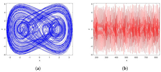
Figure 1.
(a) Complex dynamic of the Ueda oscillator, (b) Time evolution corresponding.
In this work, we are interested in introducing a discrete-time Ueda system with the use of the forward Euler method as follows:
We indicates that for , and initial conditions (ID) the trajectory corresponds to (3) a chaotic motion.
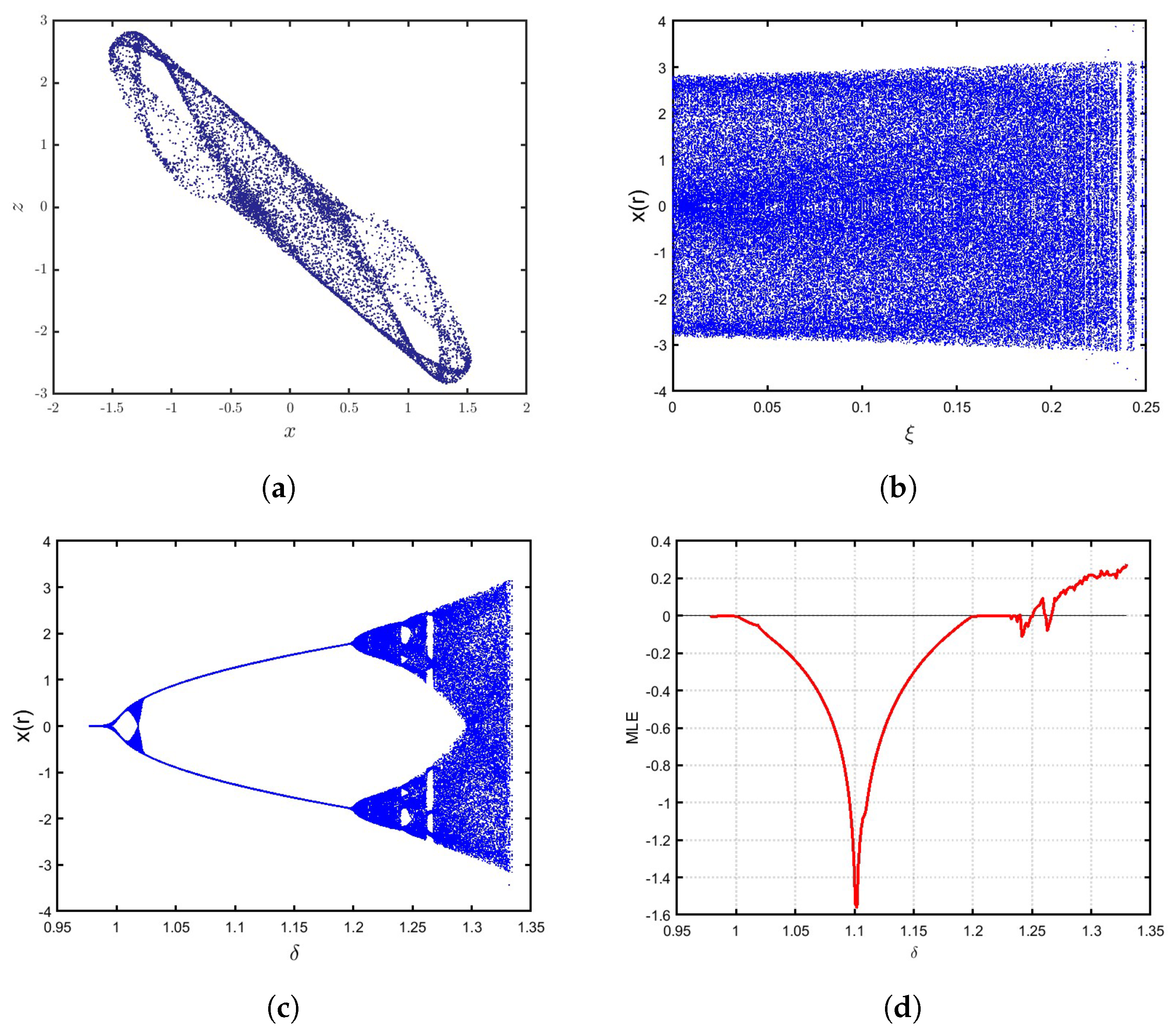
In general, studying the mechanism of the integer-order Ueda map is a fundamental tool for deep comprehension and control of the Ueda system’s chaotic behaviors. We can see that it provides a gradual evolution for tracking how chaotic behavior variation over time. In addition, the transitions between different forms and how small changes in system parameters affect the overall behavior. So, the integer-order Ueda map has been displayed to highlight a chaotic dynamic for precise and bifurcation parameters. Figure 2 shows the chaotic behavior, bifurcation plots, and the calculation of the Lyapunov exponents of the Ueda map (3) with respect to , . Illustrate the chaotic attractor with systems parameters see Figure 2a. Further, in Figure 2b,c how the bifurcation diagram generated when varying one of the parameters and fixing the other, where varies, we can observe that the behavior of the map initially has periodic trajectories then the maximum chaotic range for and . Furthermore, Figure 2d we explain that the maximum of the Lyapunov exponents (MLE) is compatible with the bifurcation plots when varies in , we can also view that if values of MLE are negative, meaning that the integer order Ueda map has periodic attractors, else are positive the map is chaotic at neighborhood of the close of interval.

In the subsequent section, our objective is to develop a fractional structure for the Ueda map. This will be achieved after providing a foundational overview of the essential ideas pertaining to discrete fractional calculus. Specifically, we’ll offer the , which represents the -th Caputo-like difference operator as defined in the work by Abdeljawad [21]. This operator will have a significant impact in formulating the fractional version of the Ueda map, allowing us to explore its dynamic behaviors under the influence of fractional-order calculus.
where , and . The fractional sum is described as [22]
Theorem 1
For , , and , for the numerical formulation of (7) written as follows:
3. The Fractional Ueda Map
This section aims to generate the fractional order version of the Ueda map based on the Caputo-like operator extending the integer-order Ueda map (3). Initially, the first-order difference Ueda map, which is represented as
Later, we use the Caputo-like fractional, for got the following 2D Ueda map:
3.1. Commensurate Case
In this subsection, the distinctive characteristics and behaviors of the commensurate fractional Ueda map are examined, a system defined by equations that all share the same fractional order. This uniformity in the fractional order provides a unique structure to the system, distinguishing it from other fractional systems with varying orders.
To systematically analyze the dynamics of this map, our approach is according to the principles established in Theorem 1, which serve as the foundational framework for our analysis, guiding the derivation of numerical methods that can accurately capture the dynamic of the commensurate Ueda map. Present the Ueda map’s mathematical formula first, explicitly detailing the equations involved. Each equation in this system is modified to incorporate the same fractional order, reflecting the commensurate nature of the system. This homogeneity in the fractional order simplifies the analysis, as we can apply uniform techniques to study the system’s behavior. Following the theoretical formulation, we derive a detailed numerical formula. This formula is crucial for implementing numerical simulations that can validate our theoretical predictions and provide insights into the complex dynamics of the Ueda map. The derivation process involves translating the continuous fractional equations into discrete counterparts that can be solved using numerical methods. By rigorously following the steps outlined in Theorem 1, we ensure that the numerical formula we derive is both accurate and efficient. This formula will be instrumental in generating phase portraits, bifurcation diagrams, and other numerical analyses highlighting the unique behaviors of the commensurate fractional Ueda map, such as potential chaotic dynamics, stability regions, and bifurcation points.
Since they relate to the bifurcation, the Lyapunov exponents are essential for illustrating chaos in fractional maps. In [24], the authors utilized the Jacobian matrix script to approximate the Lyapunov exponents for a fractional map, specifically applied to the fractional Ueda map (10). This approach effectively captures the chaotic behavior inherent in fractional-order systems.
The tangent map, integral to this analysis, incorporates discrete memory effects, which are fundamental to fractional systems. These memory effects are characterized by the system’s response depending not only on its current state but also its historical state. The discrete memory effect in the tangent map is represented by:
where
where
Then, the Lyapunov exponents given by:
for the eigenvalue of is .
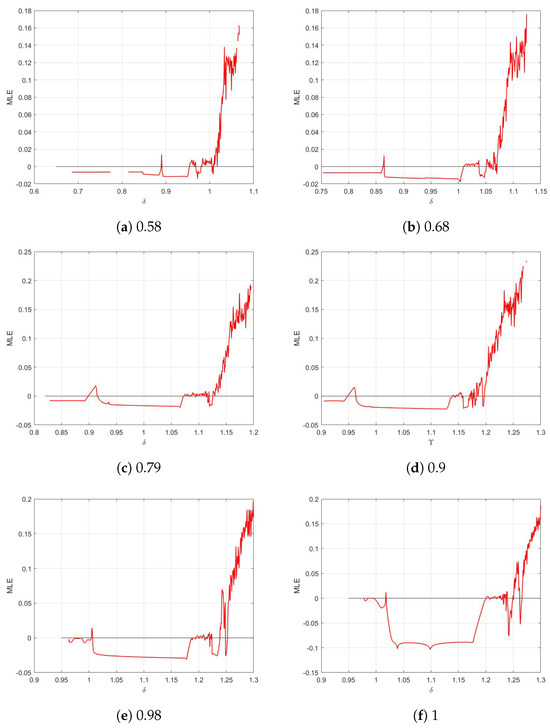
To delve into the characteristics and behavior of (10), setting (ID) as and , with fixed parameters and . Initially, we generate bifurcation diagrams of (10) against , corresponding to fractional values . This exploration is illustrated in Figure 3. It is noteworthy that when , the fractional Ueda map (10) aligns with the integer-order Ueda map (3). Observing the results, for instance, in Figure 4, we notice that the commensurate fractional Ueda map (10) exhibits two types of behavior: periodic and chaotic attractors. As the parameter increases, the periodic behavior is indicated by negative Lyapunov exponents, while higher chaotic behavior is represented by positive values. Notably, the commensurate fractional order and parameter affect the behavior of the commensurate Ueda map (10). It highlights the intricate interplay between fractional order and system parameters in shaping the dynamics of commensurate fractional systems.
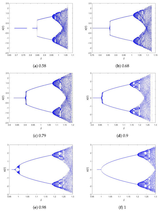
Figure 3.
Bifurcation of (10) for different and with , .
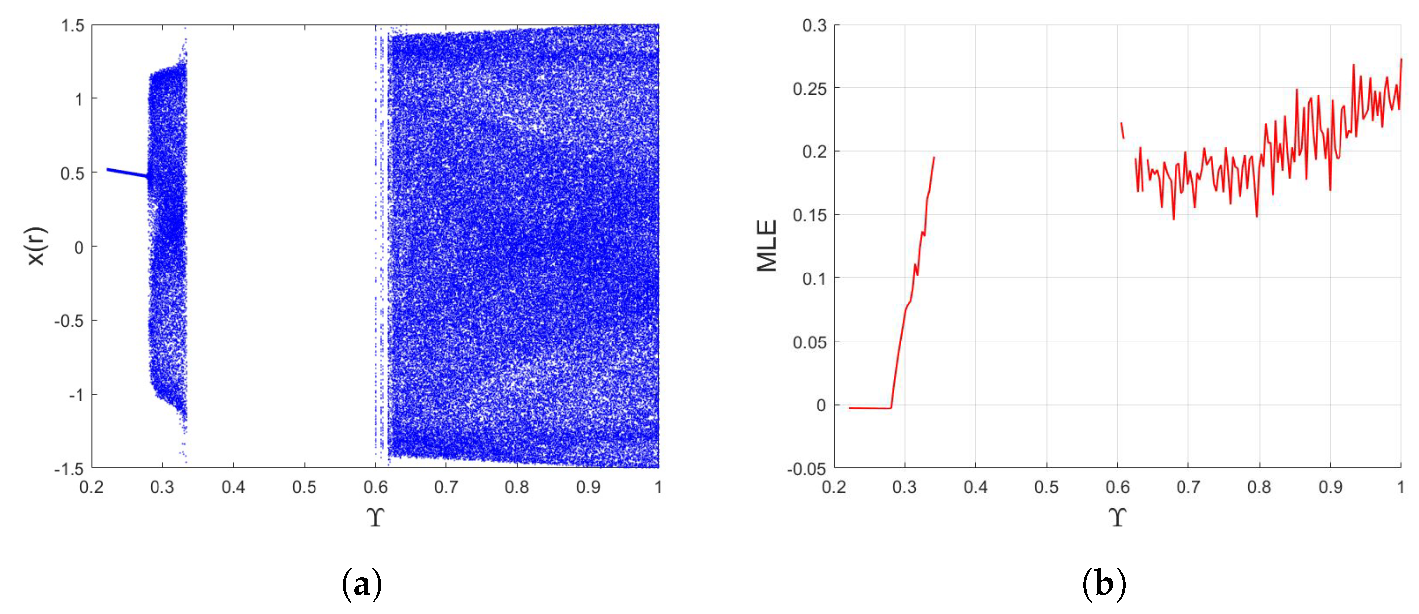
Clearly, as we vary the commensurate value with , the map (10) exhibits widespread chaotic dynamics. Moreover, when ranges from and , the fractional Ueda map (10) becomes entirely chaotic, especially as approaches 1. Additionally, within the interval , we observe a complete absence of movement in the states, indicating a state of stagnation. Conversely, when falls within the range , the fractional Ueda map (10) exhibits constant states, as depicted in Figure 5a. Similarly, the MLE in Figure 5b exhibits oscillations between positive and stable values. In some instances, certain values corresponding to bifurcation plots may disappear altogether. This observation underscores the significant impact of varying on the dynamics of the presented commensurate Ueda map. By altering , the system exhibits a wide range of dynamic behaviors, demonstrating the susceptibility of the system’s chaotic nature to alter in the fractional order. This variability highlights the complexity and richness of the dynamics in fractional maps, whereby slight variations in the fractional parameters can produce wildly disparate results.
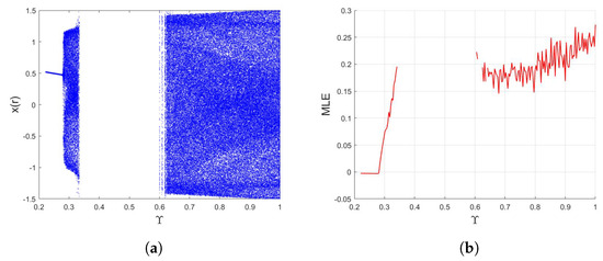
Figure 5.
(a) Bifurcation of (10) for . (b) The corresponding LEmax.
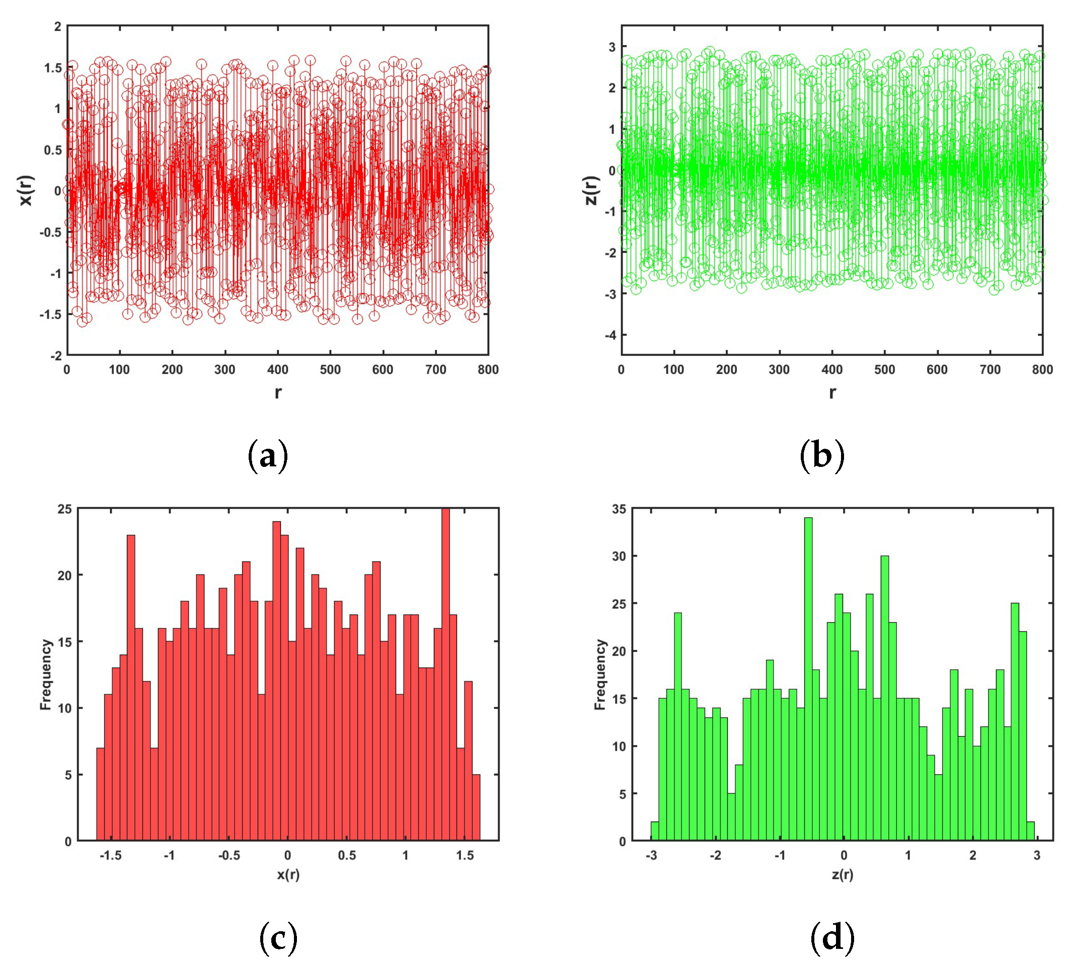
For a comprehensive illustration of the behavior, Figure 6 showcases the progression of the states x and z over time Figure 6a,b of the presented commensurate system (10) for 800 points. This visualization offers insights into the evolution of the system’s states over time, highlighting any recurring patterns or irregularities. Additionally, the histogram Figure 6c,d shows neither regular distribution of values produced by the chaotic fractional Ueda system. Its defining feature is multiple peaks indicating complicated and nonlinear dynamics. This implies a chaotic nature. Furthermore, Figure 7 presents different phase portraits for . These phase portraits provide a visual representation of the system’s attractors for varying values of the commensurate order . By examining these phase portraits, we can discern the distinct dynamical properties exhibited by the commensurate fractional Ueda map (10). Overall, these analyses demonstrate that the commensurate fractional Ueda map (10) possesses various interesting dynamical properties, including chaotic behavior, periodic motion, stagnation, and constant states, depending on the specific values of the commensurate order . These findings enrich our understanding of commensurate fractional systems and their diverse dynamics.
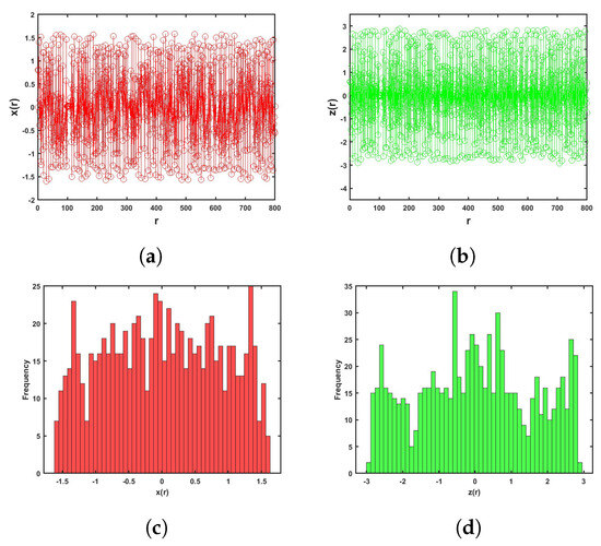
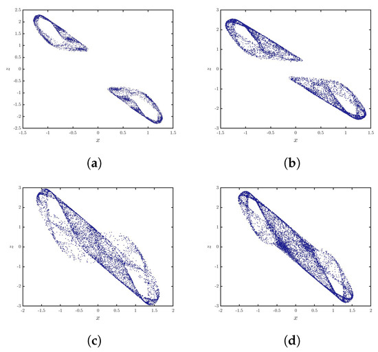
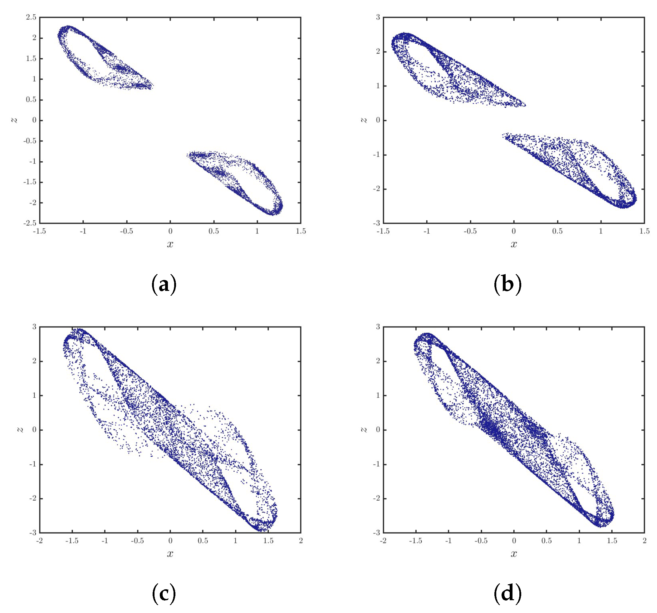
Figure 7.
Phase plane of (10) under, (a) , (b) , (c) , (d) .
3.2. Incommensurate Case
Here, the focus shifts to analyzing the behavior of a fractional Ueda map characterized by incommensurate fractional orders. This approach incorporates allocating distinct fractional values to each equation within the map, making it possible to investigate the dynamics of the map in greater detail and complexity. Introducing incommensurate fractional orders can capture a wider range of dynamics and interactions that are not possible with commensurate systems.
To rigorously study this variant, we begin by expressing the incommensurate fractional Ueda map in its formal mathematical notation. This involves specifying each equation within the system with its unique fractional order, denoted by distinct fractional values. These incommensurate values introduce a new degree of intricacy, as the behavior of each component of the system is influenced by its specific fractional order, leading to interactions and potential for rich dynamical phenomena. The formulation of the incommensurate fractional Ueda map for , is as follows:
Employing Theorem 1, we utilize the numerical formula of (16), which is outlined as follows:
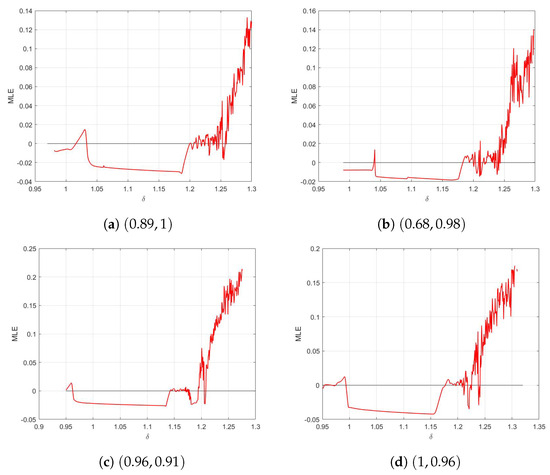
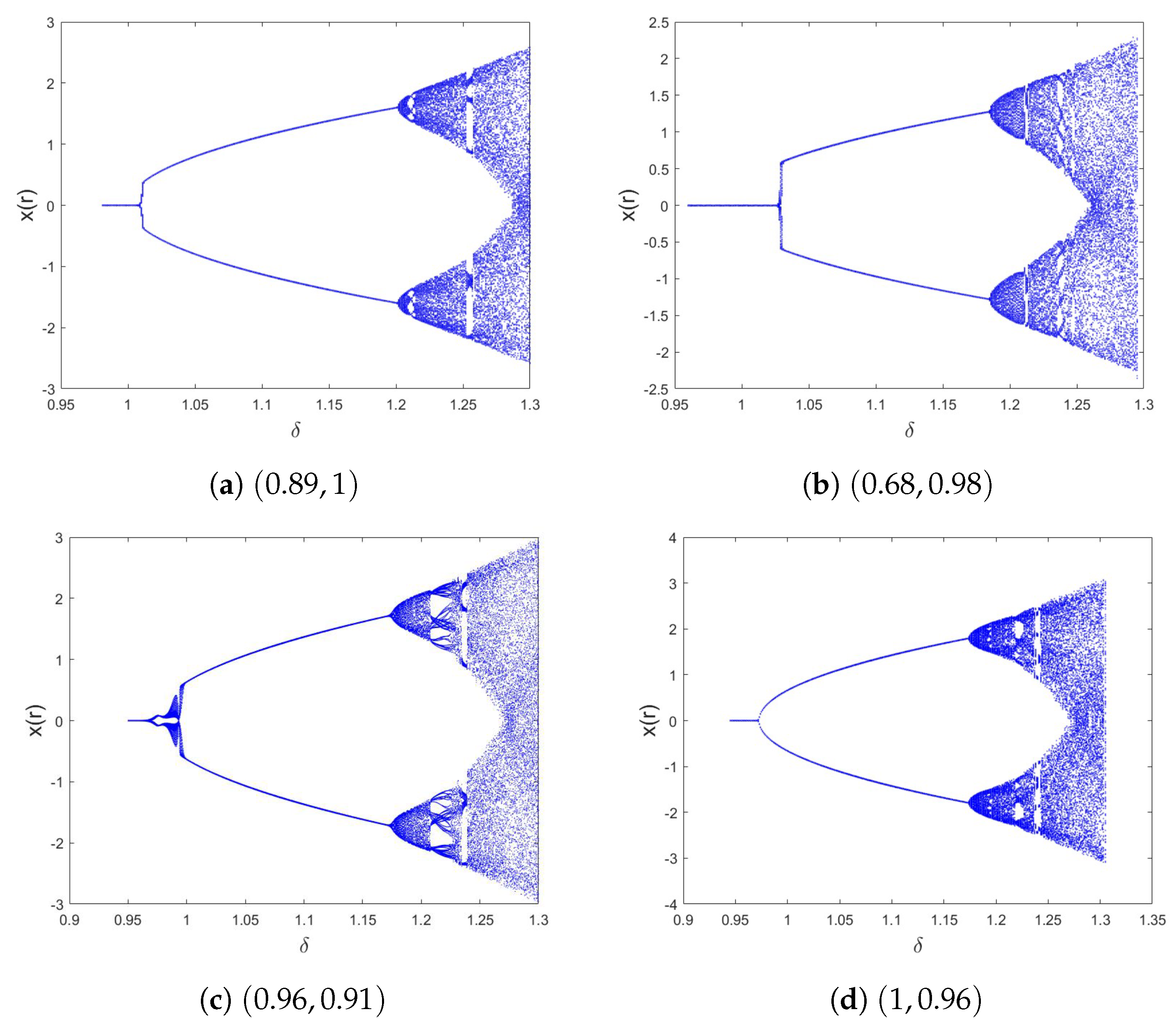
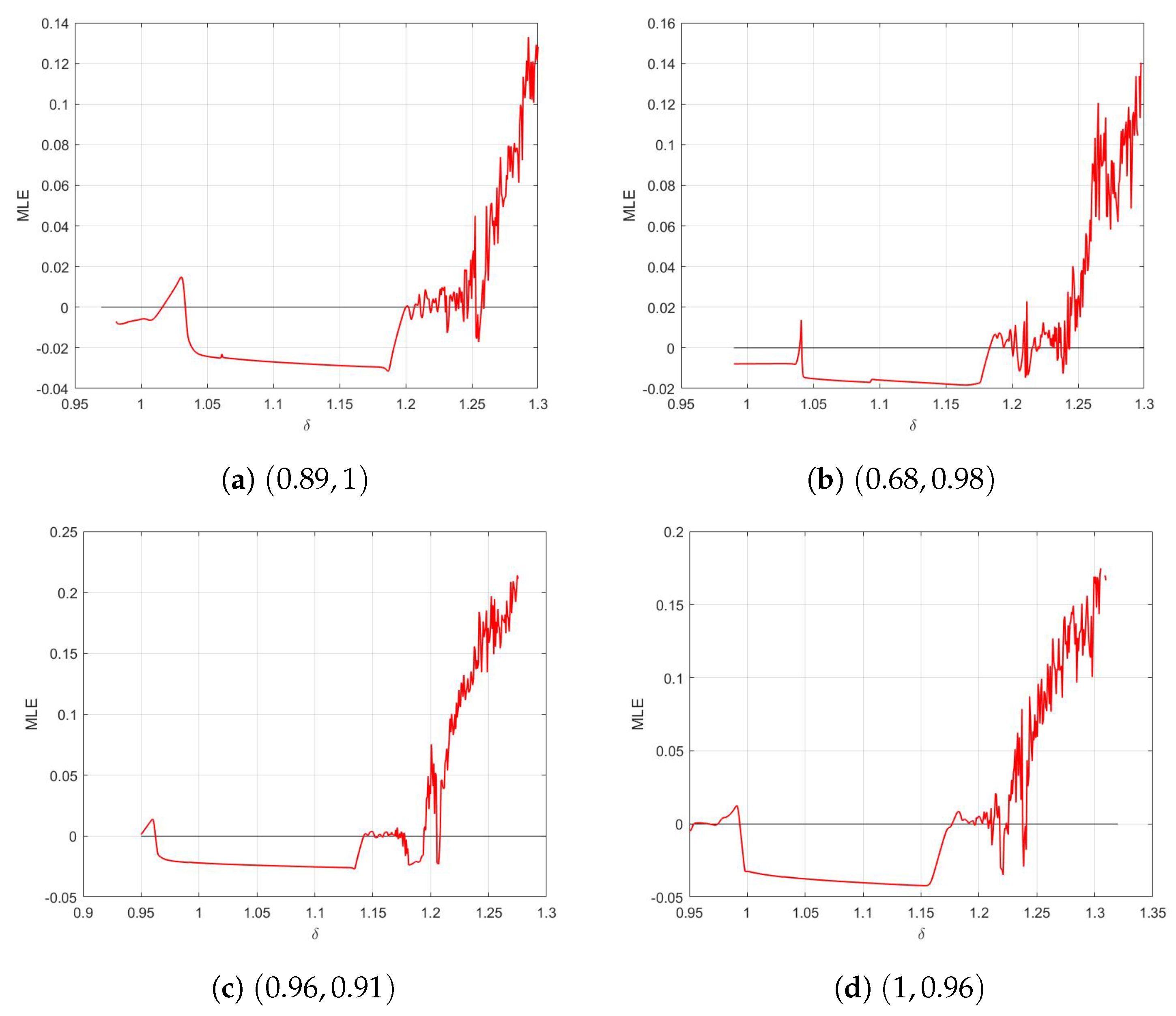
To underscore the significance of incommensurate values on the dynamics of the Ueda map (16), we present Figure 8, showcasing bifurcation and (MLE) plots for the parameter . This analysis aims to provide detailed insights into the behaviors of the incommensurate order Ueda map (16), with fixed parameters and (ID). For clarity, four bifurcation diagrams are drawn, and their corresponding MLE plots for four sets of fractional incommensurate orders: , , , and . These plots reveal distinct patterns for the four proposed orders, emphasizing the influence of fractional incommensurate orders on system behavior. As the parameter increases, trajectories of (16) evolve from periodic to chaotic behavior. Specifically, trajectories exhibit double periodicity for small values of , indicated by negative MLE values in Figure 9, while chaotic behavior emerges for larger values of , characterized by positive MLE values.
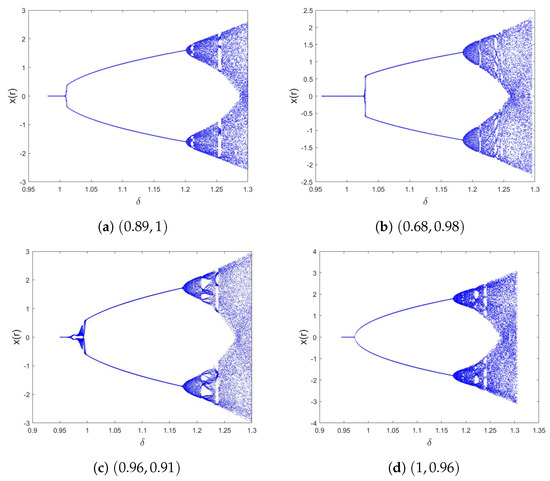
Figure 8.
Bifurcation of (16) for different and with , .
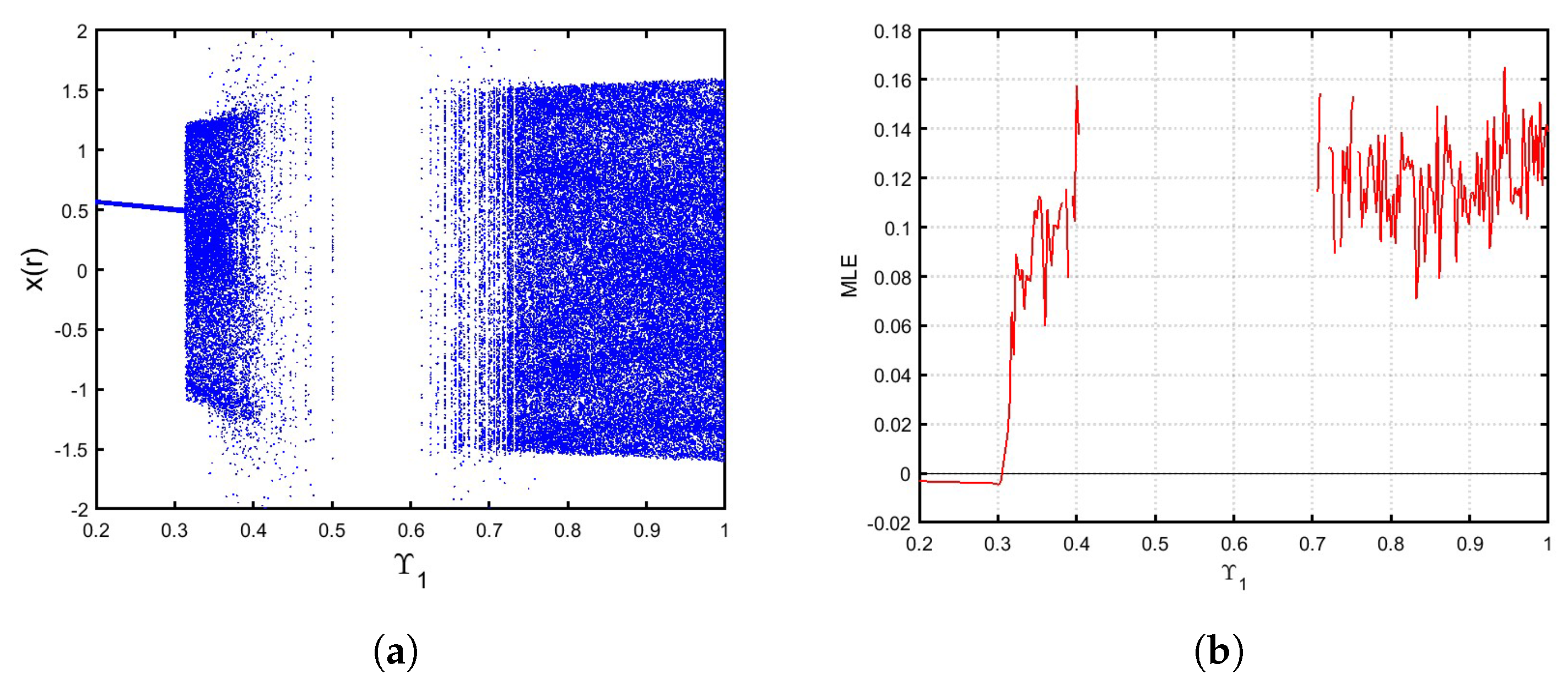
To further investigate the effects of incommensurate values on the mechanism of (16), we conducted an analysis by fixing . Specifically, we examined the bifurcation and plotted the (MLE) as varied within the interval . For this analysis, the parameters were set to and . From Figure 10, it is demonstrable that the trajectories of the incommensurate Ueda map (16) exhibit distinct behaviors depending on the value of . When falls within the intervals and , the map’s trajectories become chaotic, as indicated by the emergence of positive MLE values. Conversely, for values in the range , the system’s behavior changes dramatically. In this interval, there is a complete absence of movement in the states, resulting in constant trajectories that settle within the range . This indicates a region of parameter space where the system’s dynamics are stable and non-chaotic, with the states converging to fixed points or periodic orbits. These findings highlight the significant influence of unequal and values on the dynamic behavior of the Ueda map. The ability of the system to transition between chaotic and stable behaviors by merely adjusting the fractional orders demonstrates the complex and rich dynamics that fractional systems can exhibit. This underscores the importance of carefully selecting fractional orders in practical applications to achieve desired dynamical characteristics.

Figure 10.
(a) Bifurcationof (16) incommensurate Ueda map for and . (b) The corresponding LEmax.
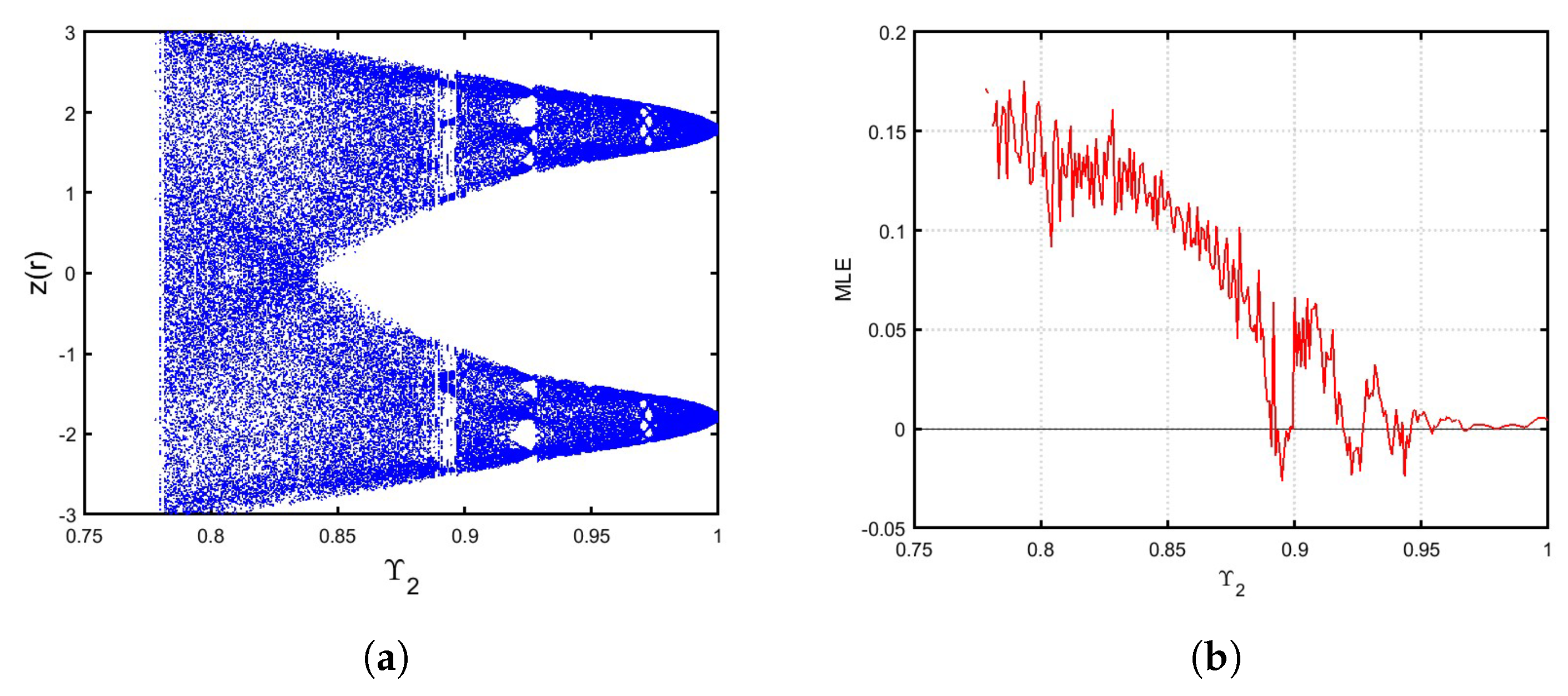
Conversely, when varying the parameter from 0.75 to 1 while keeping fixed at 0.89, the trajectories of the proposed incommensurate fractional Ueda map (16) exhibit markedly different behavior in contrast to the earlier case. As depicted in Figure 11, there is a notable increase in the chaotic region across the entire range of within the interval . This extensive chaotic behavior signifies that the incommensurate fractional Ueda map (16) becomes entirely chaotic, with the (MLE) consistently taking on positive values. This analysis demonstrates that the adjustment of has a profound impact on the map dynamics. Specifically, the interval of gives rise to chaos with periodic regions; the changes in the values of MLE from positive to negative across this interval confirm the presence and absence of chaos, indicating that the map’s sensitivity to fractional derivatives is widespread throughout the range of . The findings emphasize the significance of incommensurate orders in influencing the dynamic behavior of the system. By varying while holding constant, we observe that the system transitions from potentially stable or less chaotic states to a fully chaotic regime. This transition is critical for applications that require precise control over the system’s behavior, as it highlights the parameters that can induce or suppress chaos.
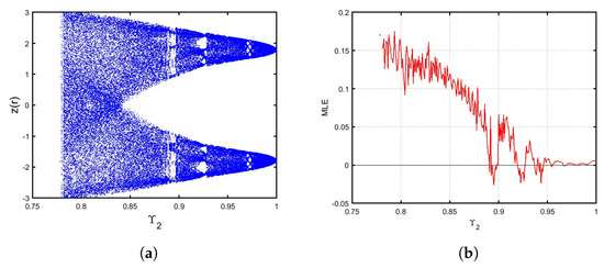
Figure 11.
(a) Bifurcationof (16) incommensurate Ueda map for ,. (b) The corresponding LEmax.
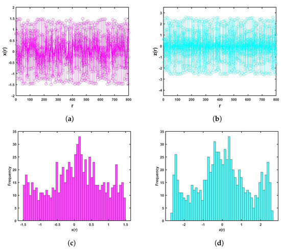
Figure 12 illustrates the numerical dynamics and histogram of the system for the specific parameter set . The figure reveals that the states exhibit chaotic behavior; this implies that the system tends to focus on particular value ranges before randomly switching to others, underscoring the system’s sensitivity to fractional orders and the complexity of its dynamics could provide additional understanding of the rich dynamics of the system.
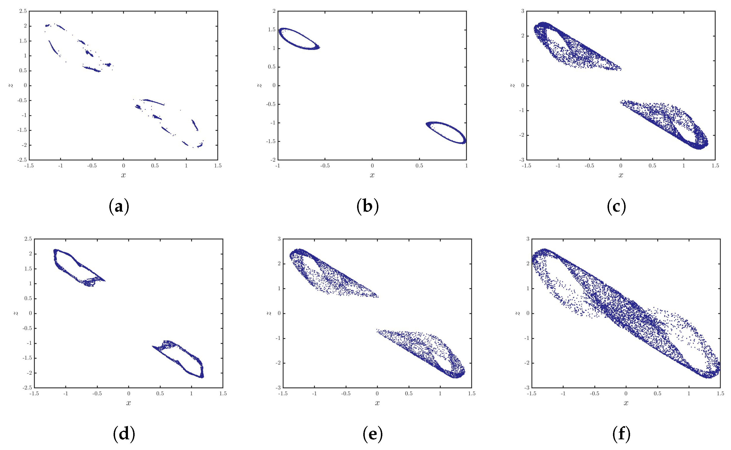
Furthermore, Figure 13 provides a comprehensive visual representation of the system’s behavior under various parameter sets. Specifically, the map (16) displays periodic portraits when the fractional orders are set to and . These periodic patterns are regions of stability where the system’s behavior is more predictable and less sensitive to initial conditions.
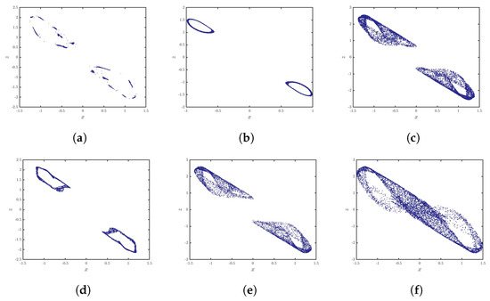
Figure 13.
Phase plane of (16) for different , (a) , (b) , (c) , (d) , (e) , (f) .
In contrast, the same map exhibits chaotic attractors for the parameter sets , , , and . These chaotic attractors highlight the system’s transition to a state of complex, unpredictable behavior. The form of these attractors changes significantly as the fractional incommensurate orders vary, demonstrating the rich diversity of the map’s dynamical responses. In summary, the results underscore the intricate.
Remark 1.
The dynamics of the fractional incommensurate Ueda map (16), as explored in Section 3.2, exhibit significant variability contrasted to the commensurate order case detailed in Section 3.1. Figures illustrate these contrasting behaviors, highlighting how fractional orders impact the system’s complexity and state variations. In Section 3.1, where commensurate fractional orders are applied to the Ueda map (10), the system displays relatively simpler dynamics. The trajectories and attractors exhibit more predictable patterns, with fewer variations in states over time. This simplicity suggests that commensurate fractional orders stabilize the system to some extent, reducing the complexity of its behavior. Conversely, Section 3.2 explores the effects of incommensurate fractional orders on the Ueda map (16). Here, the system’s behavior becomes markedly more complex and unpredictable. Figures vividly depict how different fractional order combinations lead to diverse trajectories and attractors. Incommensurate fractional orders introduce interactions among system variables, resulting in a richer spectrum of states and behaviors. The variation in fractional orders for each equation provides a deeper understanding of the complex interactions and state variations observed in the fractional Ueda map (16). Unlike the commensurate order Ueda map (10), which exhibits relatively straightforward dynamics, the incommensurate order reveals the system’s sensitivity to fractional differences. This sensitivity underscores the importance of fractional calculus in capturing and studying chaotic behaviors in dynamical systems.
4. Entropy and Complexity
In this section, our focus shifts to analyzing the complexity of the chaotic motion displayed by the fractional Ueda map. We employ both the approximate approach and the Complexity algorithm to gauge the degree of chaos within the map. Through the application of these methods, we observe that as the complexity metrics increase, there is a corresponding amplification in the chaotic region of the map. This relationship underscores the link between complexity and chaos, highlighting how the introduction of fractional-order dynamics into the Ueda map significantly enriches the map’s behavior, contributing to more pronounced and elaborate chaotic phenomena.
4.1. Approximate Entropy
In this approach, we estimate the complexity of both the commensurate Ueda map (10) and the incommensurate Ueda map (16). To achieve this, we employ the approximation Entropy (ApEn) algorithm, which is designed to effectively quantify the level of disorder and unpredictability within time series data. The (ApEn) calculation is as follows [25]:
where is given by
when represents the standard deviation and is the tolerance, we enter .
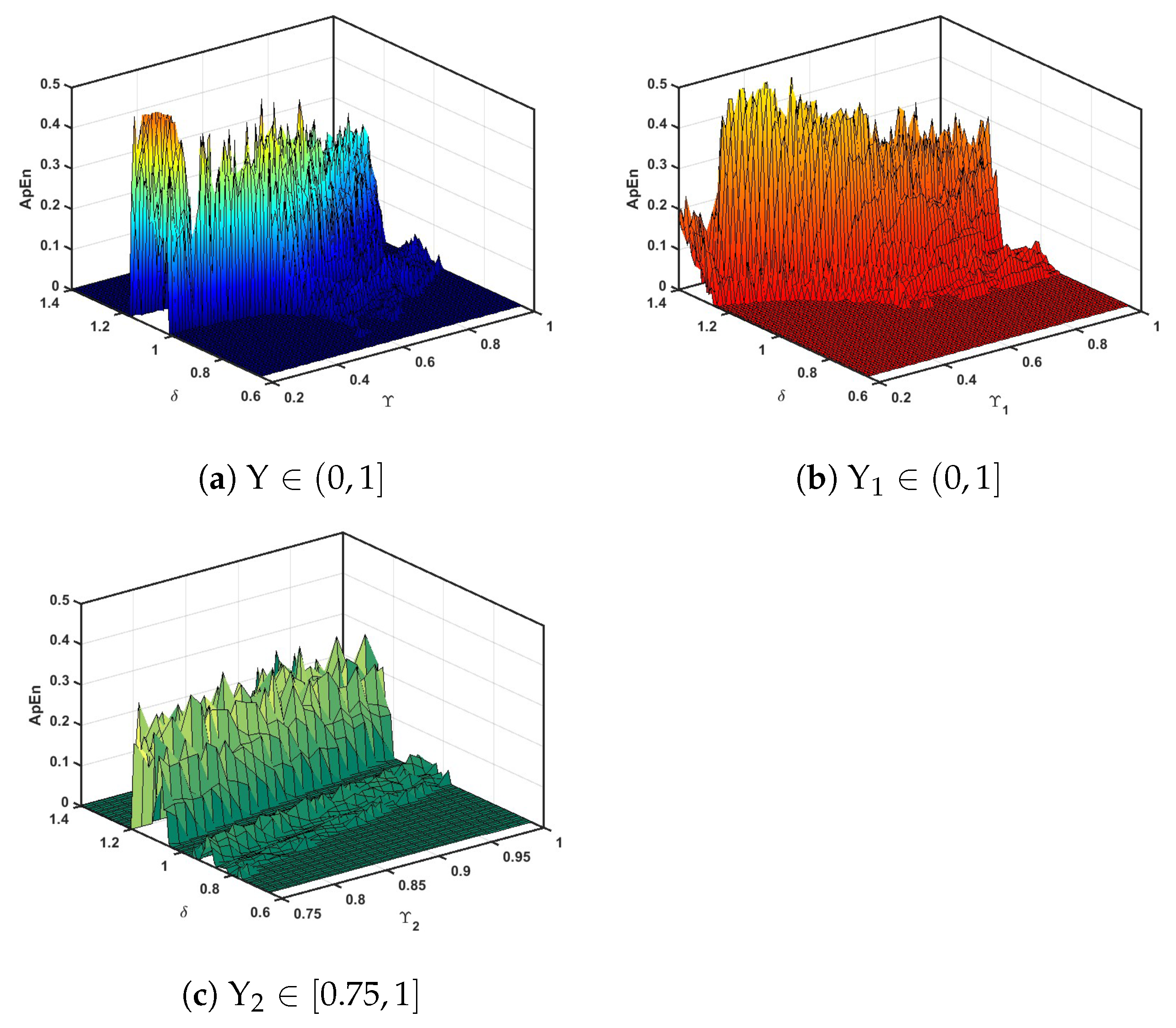
The ApEn of the commensurate Ueda map (10) and the incommensurate Ueda map (16) are shown in Figure 14. For this analysis, we set the parameter and the (ID). Such as in Figure 14a versus , Figure 14b versus for , Figure 14c versus for where are versus parameter. Both Ueda maps have higher ApEn values, indicating significant complexity, according to the ApEn computation results. A strong correlation exists between the behavior suggested by the MLE analysis and the observed complexity. The MLE values in both maps indicate that when system parameters are changed, the behavior shifts from periodic to chaotic. The presence of chaos is specifically confirmed by the positive MLE values, whereas the ApEn values offer a numerical assessment of the system’s disorder and unpredictability.

4.2. Complexity
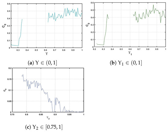
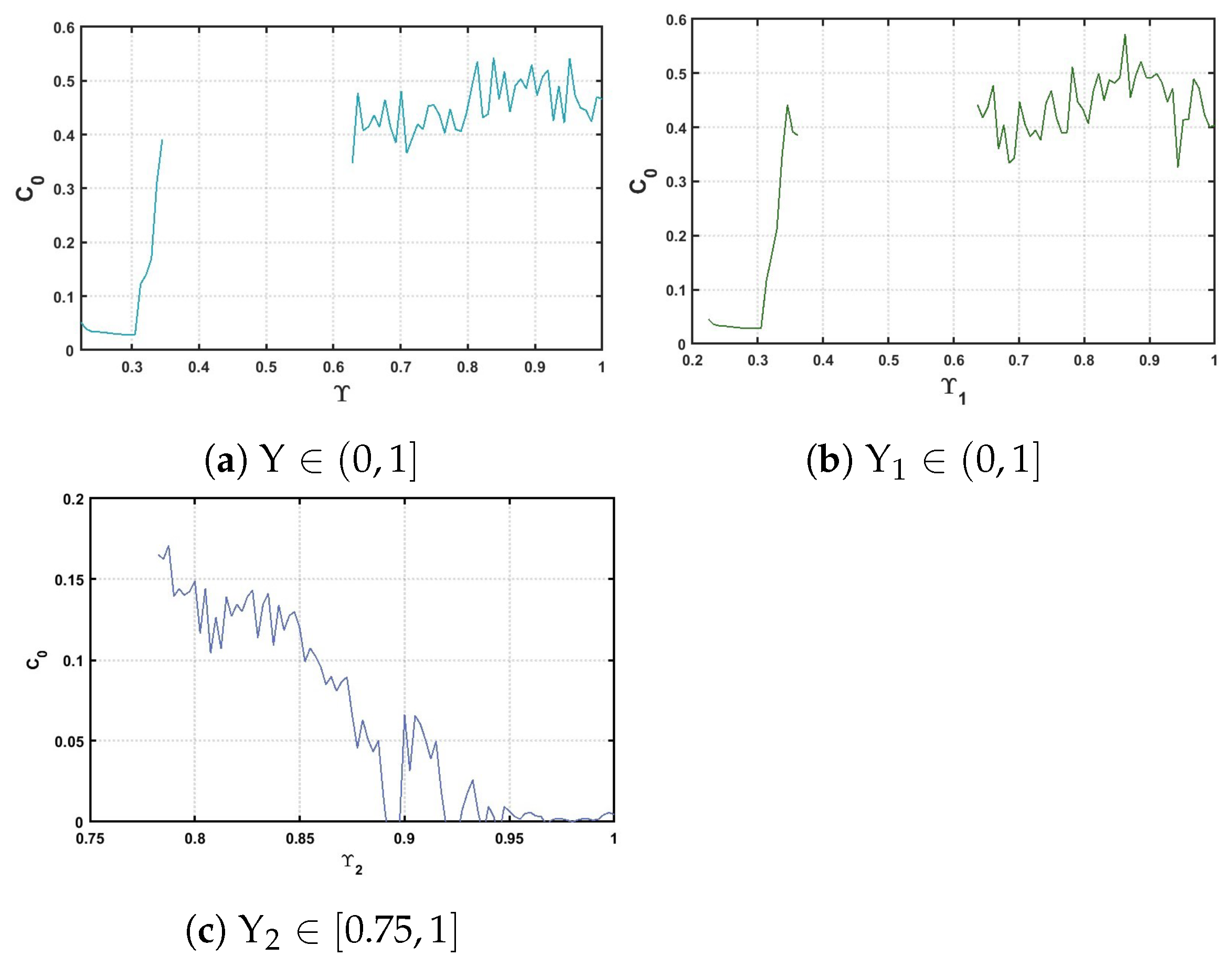
In this analysis, we employ the complexity method as described in [26] to calculate the inverse Fourier transform-derived complexity of the fractional Ueda maps S (10) and (16). This method is particularly useful for fractional-order systems as it captures the intricate and often chaotic nature of their dynamics, providing insights into the underlying behavior that might be missed by traditional analysis techniques. By applying the complexity method, we can quantify the complexity of the Ueda maps, revealing how variations in the system’s parameters influence its overall dynamic behavior. This method allows for a more thorough comprehension of the connection among the resulting system dynamics and the fractional-order properties, offering a robust tool for characterizing and analyzing complex, time-dependent behaviors in fractional-order systems.
For a series , the algorithm is detailed out of:
Step 1 the following formula determines the Fourier transform of :
Step 2 the mean square of can be characterized as: we permit
where r parameter is a control
Step 3 we implement the following expression to determine the Fourier transform’s inverse:
Step 4 to find the complexity, use the following formula:
5. Control Methods
5.1. Stabilization of the Fractional Ueda Maps
In the following sections, our focus shifts towards stabilizing the proposed Ueda fractional maps using nonlinear controllers. This effort is pivotal as it aims to steer the system towards predefined trajectories, thereby addressing and mitigating its chaotic behavior. The application of nonlinear controllers plays a crucial role in achieving stability and controlling chaotic dynamics within the Ueda fractional maps. By leveraging advanced control strategies, we aim to impose desired trajectories on the system, effectively shaping its behavior towards predictable and controlled outcomes. Stabilizing the Ueda fractional maps involves employing robust nonlinear control techniques tailored to the system’s nonlinearity and fractional dynamics. These controllers are designed to counteract the instability associated with chaotic behavior, ensuring that the system converges towards desired states or trajectories over time.
5.1.1. Stabilization of the Commensurate Version
To achieve this goal, we use the following theorem to ensure stability conditions for a commensurate fractional map.
Theorem 2
([27]). The discrete commensurate fractional system as follows
Let , and are the eigenvalues of is a matrix. There is an asymptotically stable zero equilibrium for the system should
which describes the stability conditions of the commensurate Ueda map converge to zero solution.
Then, the controller of the commensurate Ueda map is granted by
Next, the following theorem created the control law for stabilizing the commensurate Ueda map.
Theorem 3.
The commensurate Ueda map be regularized to the two-dimensional control law
where is the adaptive controller.
Proof.
The and of matrix D satisfy the conditions that follow
Consequently, the asymptotic stability of the controlled fractional Ueda map (27) is established. □
Figure 16 shows the stabilization state and histogram of the controlled (26) where with ID. Numerical analyses were conducted to ascertain the results of Theorem 5. The commensurate Ueda map shift from chaotic dynamics to a stable state is reflected in the histogram, which progressively gets more concentrated around certain values. The figures illustrated the systems approach asymptotically, which assisted to explain the stabilization results.
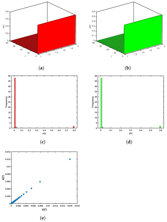
Figure 16.
Stabilization of (26) for , and , : (a,b) dynamic analysis of the states (c,d) histogram of the stable output (e) phase attractor.
5.1.2. Stabilization of the Incommensurate Version
Here, we use the following theorem to ensure stability conditions for incommensurate fractional map.
Theorem 4
([28]). Consider the system
Let , , let , and L is (LCM) of the denominators of added to , , , .
Consequently, system (30) has an asymptotically stable trivial solution.
We introduce the control of the incommensurate Ueda map as the following
The next theorem presents the control laws aimed at stabilizing the incommensurate Ueda map.
Theorem 5.
When suitable two-dimensional control laws are constructed in the following
It is achieves the stabilization the incommensurate Ueda map at the equilibrium.
Proof.
So
where , and
for ,
⇔
Therefore, can be inferred. Consequently, (33) is asymptotically stable in the direction of the point. □
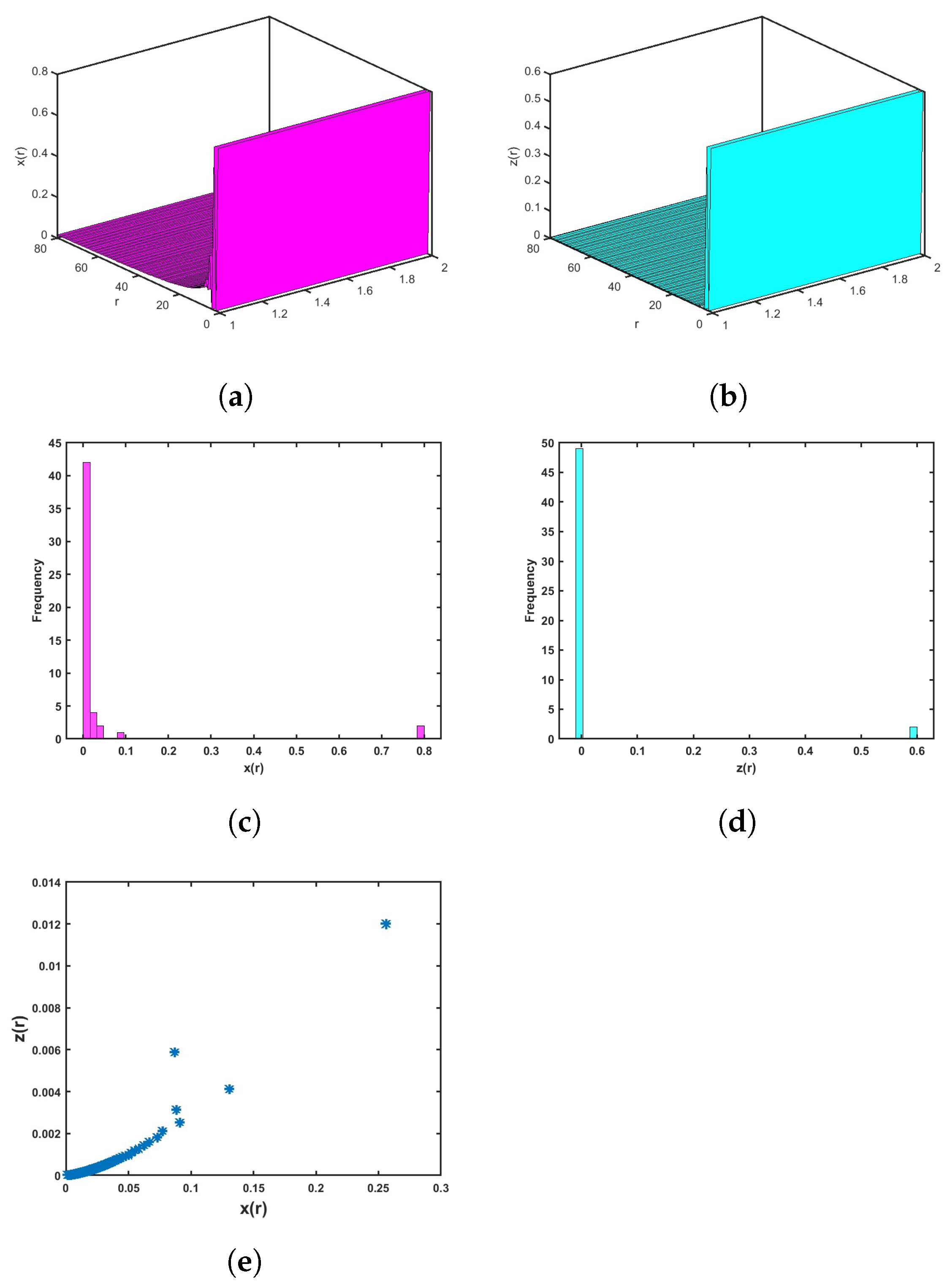
For the results to be validated numerically, Figure 17 shows the stabilization states and histogram of the controlled incommensurate map (33) for with (ID). An asymptotically stable incommensurate ueda map’s deterministic character is reflected in this histogram behavior. Strong damping in the system minimizes dynamic disturbances and illustrates how the map converges towards .
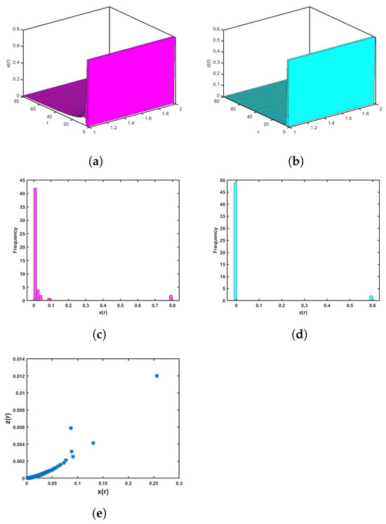
Figure 17.
Stabilization of (33) for , with , : (a,b) dynamic analysis of the states (c,d) histogram of the stable output (e) phase attractor.
5.2. Synchronization Between Fractional Ueda Map
In this part, our aim is to delve into the process of achieving synchronization between two 2D fractional Ueda maps. Synchronization plays a pivotal role in minimizing the disparity between a master map and a slave map, ensuring that their trajectories converge toward each other. Our approach begins by defining the master map using the commensurate fractional Ueda map (10), which serves as the reference system. Meanwhile, the slave Ueda map is structured as follows:
The synchronization controllers are denoted by and . The fractional error map is provided as:
where the synchronization error described as
when , .
Theorem 6.
Proof.
Asper Theorem 2, the eigenvalues of B can be examined to ascertain the stability of the error system (39). The eigenvalues are and ; for the system to be asymptotically stable, these eigenvalues must satisfy the stability condition, which requires that both have negative real parts. Given the parameters and and , we calculate the eigenvalues as follows: Since both eigenvalues are negative, the stability requirement is met. This ensures the zero solution of the error system (39) is asymptotically stable. Consequently, the synchronization between the master Ueda (10) and the slave Ueda (38) maps is achieved. □
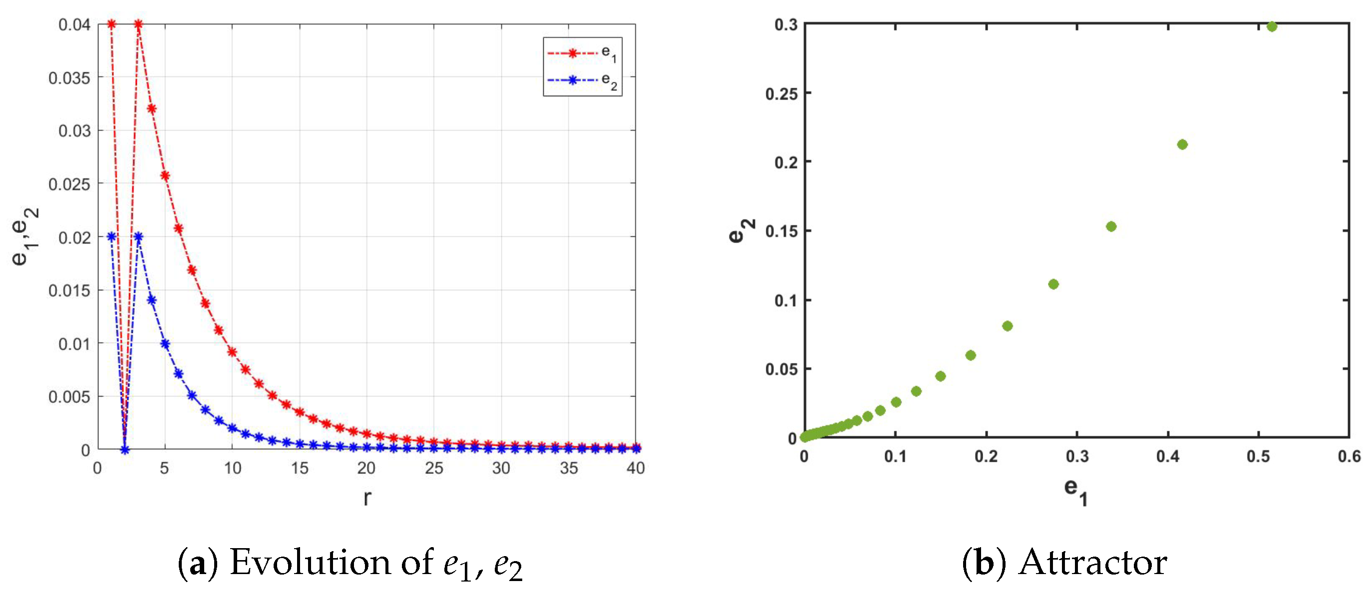
To validate these theoretical results, we conduct numerical simulations. For the simulations, we select specific parameters: the commensurate fractional order , , and In Figure 18, the stabilization of the error map (39) is depicted. The graph clearly shows that the errors and converge to zero over time. This convergence indicates that the synchronization between the master and slave Ueda maps has been successfully achieved, as the difference between their states diminishes to zero. This numerical validation supports our research findings and demonstrates the practicality of the proposed synchronization schema under the specified conditions. The synchronization is crucial for ensuring that the dynamic of the slave map closely follows that of the master map, which is crucial for many control applications.
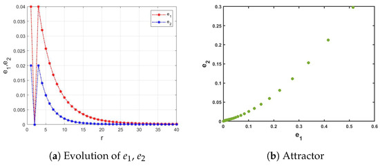
Figure 18.
Synchronization of the fractional error map (39).
6. Conclusions and Future Works
This article investigates a variant of the Ueda chaotic map characterized by commensurate and incommensurate Caputo-like fractional orders. The analysis demonstrates that the Ueda map exhibits robust chaotic behavior across a wide range of the bifurcation parameter and fractional values . By using tools like Lyapunov exponents, bifurcation diagrams, and complexity measures like complexity and approximation Entropy (ApEn), the chaotic behavior of the map is rigorously established in both commensurate and incommensurate cases.
In addition to exploring the chaotic dynamics, we propose control laws designed to stabilize and synchronize the Ueda map. These control strategies effectively guide the trajectories to a stable state, showcasing the practical applicability of chaos theory in managing complex systems. This has significant implications for real-world applications, including secure communication, neural networks, and electronic systems.
Future work will focus on leveraging the fractional Ueda map’s chaotic properties for developing advanced encryption techniques and enhancing neural network architectures. The rich dynamics of the Ueda map offer promising avenues for improving data security, generative modeling, and predictive capabilities in various domains.
Author Contributions
Conceptualization, A.O. and G.G.; Data curation, L.D. and A.O.; Formal analysis, G.G. and A.H.; Funding acquisition, S.M., A.O. and G.G.; Investigation, A.O.; Methodology, L.D.; Project administration, A.H.; Resources, L.D. and A.O.; Software, G.G. and S.M.; Supervision, A.O.; Validation, G.G.; Visualization, S.M.; Writing—original draft, L.D.; Writing—review & editing, A.H. All authors have read and agreed to the published version of the manuscript.
Funding
This research received no external funding.
Data Availability Statement
The original contributions presented in this study are included in the article. Further inquiries can be directed to the corresponding author.
Acknowledgments
This work is supported by Ajman University Internal Research Grant No. [DRGS Ref. 2024-IRG-HBS-4].
Conflicts of Interest
The authors declare no conflict of interest.
References
- He, C.H.; Tian, D.; Moatimid, G.M.; Salman, H.F.; Zekry, M.H. Hybrid Rayleigh-van der pol-duffing oscillator: Stability analysis and controller. J. Low Freq. Noise, Vib. Act. Control 2022, 41, 244–268. [Google Scholar] [CrossRef]
- Ueda, Y. Randomly transitional phenomena in the system governed by Duffing’s equation. J. Stat. Phys. 1979, 20, 181–196. [Google Scholar] [CrossRef]
- Guckenheimer, J.; Holmes, P. Nonlinear Oscillations, Dynamical Systems, and Bifurcations of Vector Fields; Springer Science & Business Media: Berlin/Heidelberg, Germany, 2013; Volume 42. [Google Scholar]
- Zhang, X.; Li, C.; Chen, Y.; Herbert, H.C.; Lei, T. A memristive chaotic oscillator with controllable amplitude and frequency. Chaos Solitons Fractals 2020, 139, 110000. [Google Scholar] [CrossRef]
- Houas, M.; Samei, M.E.; Sundar Santra, S.; Alzabut, J. On a Duffing-type oscillator differential equation on the transition to chaos with fractional q-derivatives. J. Inequalities Appl. 2024, 2024, 12. [Google Scholar] [CrossRef]
- Kassim, S.; Hamiche, H.; Djennoune, S.; Bettayeb, M. A novel secure image transmission scheme based on synchronization of fractional-order discrete-time hyperchaotic systems. Nonlinear Dyn. 2017, 88, 2473–2489. [Google Scholar] [CrossRef]
- Jain, K.; Aji, A.; Krishnan, P. Medical image encryption scheme using multiple chaotic maps. Pattern Recognit. Lett. 2021, 152, 356–364. [Google Scholar] [CrossRef]
- Alhamadani, B.N. Implement image encryption on chaotic and discrete transform domain encryption. Inform. J. Appl. Mach. Electr. Electron. Comput. Sci. Commun. Syst. 2021, 2, 36–41. [Google Scholar]
- Sun, K.; Duo Li-kun, A.; Dong, Y.; Wang, H.; Zhong, K. Multiple coexisting attractors and hysteresis in the generalized Ueda oscillator. Math. Probl. Eng. 2013, 2013, 256092. [Google Scholar] [CrossRef]
- Huang, L.L.; Baleanu, D.; Wu, G.C.; Zeng, S.D. A new application of the fractional logistic map. Rom. J. Phys. 2016, 61, 1172–1179. [Google Scholar]
- Ostalczyk, P. The non-integer difference of the discrete-time function and its application to the control system synthesis. Int. J. Syst. Sci. 2000, 31, 1551–1561. [Google Scholar] [CrossRef]
- Ferreira, R.A. Discrete Fractional Calculus and Fractional Difference Equations; Springer: Cham, Switzerland, 2022. [Google Scholar]
- Tavazoei, M.; Asemani, M.H. On robust stability of incommensurate fractional-order systems. Commun. Nonlinear Sci. Numer. Simul. 2020, 90, 105344. [Google Scholar] [CrossRef]
- Fiaz, M.; Aqeel, M.; Marwan, M.; Sabir, M. Integer and fractional order analysis of a 3D system and generalization of synchronization for a class of chaotic systems. Chaos Solitons Fractals 2022, 155, 111743. [Google Scholar] [CrossRef]
- Ouannas, A.; Batiha, I.M.; Pham, V.T. Fractional discrete chaos: Theories, methods and applications. In World Scientific; World Scientific Publishing: Singapore, 2023; Volume 3. [Google Scholar]
- Zhang, Y.; Li, J.; Zhu, S.; Zhao, H. Bifurcation and chaos detection of a fractional Duffing-van der Pol oscillator with two periodic excitations and distributed time delay. Chaos Interdiscip. J. Nonlinear Sci. 2023, 33, 083153. [Google Scholar] [CrossRef]
- Ouannas, A.; Khennaoui, A.A.; Oussaeif, T.E.; Pham, V.T.; Grassi, G.; Dibi, Z. Hyperchaotic fractional Grassi-Miller map and its hardware implementation. Integration 2021, 80, 13–19. [Google Scholar] [CrossRef]
- Wang, Z.R.; Shiri, B.; Baleanu, D. Discrete fractional watermark technique. Front. Inf. Technol. Electron. Eng. 2020, 21, 880–883. [Google Scholar] [CrossRef]
- Ouannas, A.; Khennaoui, A.A.; Momani, S.; Pham, V.T. The discrete fractional duffing system: Chaos, 0-1 test, C complexity, entropy, and control. Chaos Interdiscip. J. Nonlinear Sci. 2020, 30, 083131. [Google Scholar] [CrossRef] [PubMed]
- Ramroodi, N.; Tehrani, H.A.; Skandari, M.N. Numerical behavior of the variable-order fractional Van der Pol oscillator. J. Comput. Sci. 2023, 74, 102174. [Google Scholar] [CrossRef]
- Abdeljawad, T. On Riemann and Caputo fractional differences. Comput. Math. Appl. 2011, 62, 1602–1611. [Google Scholar] [CrossRef]
- Atici, F.M.; Eloe, P. Discrete fractional calculus with the nabla operator. Electron. J. Qual. Theory Differ. Equ. [Electron. Only] 2009, 62, 12. [Google Scholar] [CrossRef]
- Wu, G.C.; Baleanu, D. Discrete fractional logistic map and its chaos. Nonlinear Dyn. 2014, 75, 283–287. [Google Scholar] [CrossRef]
- Wu, G.C.; Baleanu, D. Jacobian matrix algorithm for Lyapunov exponents of the discrete fractional maps. Commun. Nonlinear Sci. Numer. Simul. 2015, 22, 95–100. [Google Scholar] [CrossRef]
- Richman, J.S.; Moorman, J.R. Physiological time-series analysis using approximate entropy and sample entropy. Am. J.-Physiol. Circ. Physiol. 2000, 278, H2039–H2049. [Google Scholar] [CrossRef] [PubMed]
- Shen, E.-H.; Cai, Z.-J.; Gu, F.-J. Mathematical foundation of a new complexity measure. Appl. Math. Mech. 2005, 26, 1188–1196. [Google Scholar]
- Čermák, J.; Győri, I.; Nechvátal, L. On explicit stability conditions for a linear fractional difference system. Electron. J. Qual. Theory Differ. Equ. [Electron. Only] 2015, 18, 651–672. [Google Scholar] [CrossRef]
- Shatnawi, M.T.; Djenina, N.; Ouannas, A.; Batiha, I.M.; Grassi, G. Novel convenient conditions for the stability of nonlinear incommensurate fractional-order difference systems. Alex. Eng. J. 2022, 61, 1655–1663. [Google Scholar] [CrossRef]


Disclaimer/Publisher’s Note: The statements, opinions and data contained in all publications are solely those of the individual author(s) and contributor(s) and not of MDPI and/or the editor(s). MDPI and/or the editor(s) disclaim responsibility for any injury to people or property resulting from any ideas, methods, instructions or products referred to in the content. |
© 2025 by the authors. Licensee MDPI, Basel, Switzerland. This article is an open access article distributed under the terms and conditions of the Creative Commons Attribution (CC BY) license (https://creativecommons.org/licenses/by/4.0/).