Article

Information Perception Adaptive Filtering Algorithm Sensitive to Signal Statistics: Theory and Design

1
College of Electronic and Information, Southwest Minzu University, Chengdu 610041, China
2
Key Laboratory of Electronic and Information Engineering, State Ethnic Affairs Commission, Chengdu 610041, China
3
School of Mechanical and Power Engineering, Henan Polytechnic University, Jiaozuo 454003, China
4
Department of Biomedical Engineering, New Jersey Institute of Technology, Newark, NJ 07102, USA
*
Author to whom correspondence should be addressed.
Mathematics 2025, 13(20), 3294; https://doi.org/10.3390/math13203294
Submission received: 5 September 2025 / Revised: 9 October 2025 / Accepted: 13 October 2025 / Published: 15 October 2025

Abstract

To address the challenges of information perception, this paper proposes a novel adaptive filtering algorithm. The algorithm is built upon an asymmetric cost function. It incorporates an information perception strategy, referred to as the information perception adaptive filtering (IPAF) algorithm, in which the parameters of the cost function are directly linked to statistical characteristics. The key advantage of this algorithm is that its parameters can be adaptively adjusted in real-time according to higher-order statistical properties in different environments, thereby overcoming the limitations of traditional fixed-parameter algorithms. A comprehensive performance analysis of the IPAF algorithm is presented, including convergence analysis, mean square deviation analysis, and computational complexity analysis. Extensive simulation experiments and evaluations of real datasets demonstrate that the IPAF algorithm achieves reliable information perception with excellent robustness.

1. Introduction

In the wake of the Internet of Things and rapid industrialization, there is a growing demand for efficient, accurate, and robust information perception, as well as intelligent collaboration across various fields. Information perception is increasingly reflected in diverse application domains, such as 5G communication systems [1], industrial inspection and maintenance [2], and radar signal processing [3]. For example, radar systems represent typical intelligent platforms that must effectively sense and track targets within surveillance areas. However, in practical scenarios, the presence of nonlinear and non-Gaussian interference, dynamic environmental variations, and even malicious disturbances poses significant challenges to achieving reliable information perception [4]. These challenges underscore the urgent need for effective theoretical and algorithmic frameworks that can ensure robust and accurate perception under complex and uncertain conditions. In this context, parameter estimation emerges as a fundamental approach for extracting critical information from noisy and uncertain environments. Since parameter estimation is inherently and closely linked with adaptive filtering (AF), advances in AF theory and methodology offer a powerful avenue to address the challenges of information perception [5].
AFs have achieved wide application in various fields of signal processing [6]. Taking linear AFs as an example, their applications include antenna array processing of multichannel signals and beamforming in system identification [7,8,9]. To address these practical challenges, scholars have conducted extensive research on classical AF algorithms, including the least mean square (LMS) algorithm [10,11], the affine projection algorithm (APA) [12,13], and the recursive least-squares (RLS) algorithm [14,15]. Due to its computational simplicity and ease of implementation, LMS has been widely applied in areas such as system identification, channel equalization, and noise cancellation [16,17]. To further enhance the performance of LMS in practical applications, researchers have proposed various improved algorithms based on the original framework, including the normalized LMS (NLMS) algorithm [18] and the variable step-size LMS (VSS-LMS) algorithm [19]. Researchers have also developed several excellent processing methods in the nonlinear domain, including spline adaptive filtering (SAF) [20], a cascaded filter with a hierarchical design integrating the functional link artificial neural network (FLANN) and Legendre neural network (LNN) [21], and the constrained recursive kernel risk-sensitive loss (CRKRSL) [22]. Ideally, classical AF algorithms usually achieve fast convergence and good steady-state performance. However, in real-world scenarios, signals are often subject to more complex non-Gaussian disturbances, such as those caused by lightning, industrial machinery, and underwater acoustic noise. Under such conditions, the performance of classical AF algorithms is severely challenged.
To further optimize the performance of AF algorithms, researchers have proposed various solutions. Among these, the choice of an appropriate cost function has become a significant research focus, as selecting a suitable cost function in different environments plays a crucial role in determining algorithm performance. Consequently, many AF algorithms have been developed based on various cost functions. Based on the minimum mean p-power error (MPE) criterion, the least mean p-power (LMP) algorithm achieves comprehensive performance [23]. The least mean fourth (LMF) algorithm, which employs the fourth-order error moment as the cost function, achieves faster convergence [24]. Wang has designed a variable-scale-factor filter using the logarithmic hyperbolic cosine function, referred to as LHCAF [25]. At the same time, Liang has employed the same function to propose a constrained minimum lncosh AF algorithm capable of coping with non-Gaussian impulsive noise [26]. A novel diffusion adaptive estimation algorithm is proposed from an M-estimator perspective, which is called the diffusion Fair (DFair) AF algorithm. [27]. Additionally, AF algorithms that incorporate the cost function into an inverse tangent framework have been proposed in [28]. Simulations of algorithms developed within a sigmoid framework for system identification and acoustic echo cancellation have demonstrated superior performance [29]. More recently, a robust half-quadratic criterion (HQC) AF algorithm utilizing a convex cost function has been introduced, offering a more efficient performance surface compared with conventional methods [30]. To further enhance steady-state convergence behavior under impulsive noise, researchers have proposed the generalized robust logarithmic family (GRLF) framework, which incorporates relative logarithmic cost functions and minimum variance constraints (MVCs), for the design of AF [31]. A generalized soft-root-sign (GSRS) function and the corresponding GSRS adaptive filter (AF) are proposed in [32].
Unfortunately, most existing approaches that enhance the performance of AF algorithms through various cost functions primarily focus on the characteristics of interference, while largely neglecting the characteristics of the system’s input signals. It is essential to emphasize that input, output, system state, and interference are all critical components of a system. In many application domains—for example, channel equalization in wireless electromagnetic wave transmission—only input, output, and interference are typically considered. However, in deterministic systems, a strong correlation exists between input, interference, and output. Thus, constructing the cost function in adaptive estimation theory solely from the estimation error, or designing it merely based on the symmetry of the statistical distribution of interference, leads to an incomplete formulation. To address this issue, this paper proposes constructing the cost function jointly from the input and interference. Specifically, higher-order statistical properties distinguish different inputs and noise environments, and the loss parameter in the cost function is mapped to these properties. Based on this formulation, we design a novel adaptive estimation algorithm that can effectively perceive information under varying input and noise conditions.
The main contributions of this paper are as follows:
(1)
By combining an asymmetric loss function with an information perception strategy, we propose a novel AF algorithm, termed the IPAF algorithm.
(2)
We provide a detailed performance analysis of the IPAF algorithm, including convergence analysis, mean square deviation analysis, and computational complexity analysis.
(3)
We validate the effectiveness of the proposed information perception strategy. The IPAF algorithm is compared with other robust algorithms under four different environments—Gaussian inputs, non-Gaussian inputs with symmetric noise, and asymmetric noise—demonstrating its superior performance.
(4)
We further validate the performance of the proposed algorithm on real datasets.
The real-time perception capability targeted by the filtering algorithm designed in this paper aims to differentiate itself from traditional fixed-parameter filtering algorithms. Its cost function can adaptively adjust based on higher-order statistical characteristics observed across various environments. The remainder of this paper is organized as follows. Section 2 describes the algorithm design. Section 3 presents the detailed performance analysis. Section 4 reports the simulation results, and Section 5 concludes the paper.
The following table provides annotations for relevant variables and symbols in this paper. Scalars in this paper are denoted by standard italic type, while vectors and matrices are represented in bold type. Notes are arranged in the order of their appearance in the main text. Annotations follow the order of appearance in the text.
(·)T
α
β
|·|
E[·]
λmax
I
R
||·||
Tr(·)
Transpose operator
Skewness mapping parameters
Kernel mapping parameters
Absolute value operator
Mathematical expectation operator
Largest eigenvalue of a matrix
Identity matrix
Autocorrelation matrix
Euclidean norm of a vector
Trace of a matrix

2. Algorithm Design

This chapter introduces an AF algorithm with information perception capabilities that integrates robustness and adaptive adjustment features, enabling proactive responses to varying environments. The system input signal is represented as X(i) = [x(i), x(i − 1), …, x(iL + 1)]T, where L is the filter length. The weight vector is ω(i) = [ω(0), ω(1), …, ω(L − 1)]T. where the output of the filter at moment i is:
y i = ω T i X i
The expectation signal is expressed as:
d i = ω 0 T X i + v ( i )
where ω0 is defined as the filter optimal weight vector, v(i) is zero-mean Gaussian noise, and the input signal X(i) is a zero-mean smooth Gaussian random sequence. The error signal is defined as:
e i = d i y ( i )
The cost function is shown in Equation (4):
J e ( i ) = 1 1 1 + β e ( i ) 2 exp α e ( i )
This cost function, inspired by [33], exhibits several key characteristics: (1) robustness against outliers and noise, (2) smoothness, boundedness, and continuity, and (3) two adjustable shape parameters. These properties make it effective in resisting outliers and noise while maintaining smoothness, which ensures well-defined gradients—an advantage for designing filtering algorithms. Figure 1 illustrates the function and its gradient across varying parameter values. Figure 1a,b present images of the function and its gradient for varying values of α, illustrating that the cost function’s asymmetry intensifies as α increases. Similarly, Figure 1c,d depict the function and gradient images for different β values, revealing that the cost function steepens with increasing β.
Contemporary robust algorithms often rely on fixed-parameter mechanisms, limiting their adaptability to specific environments. To address this limitation, we introduce information perception parameters by leveraging the two parameters in the cost function of Equation (4). These parameters are correlated with the statistical characteristics of varying input and noise environments: parameter α is linked to the skewness of different noises, while β relates to the kurtosis of diverse input signals. This approach differentiates environments based on third-order and fourth-order statistical distances, as illustrated in Equations (5) and (6):
α = α m i n + c · γ α m i n , α m a x
β = β m i n + d · κ β m i n , β m a x
Parameter α is associated with the skewness of noise under different conditions, whereas β corresponds to the kurtosis of the input signal. The third- and fourth-order statistical measures enable differentiation between Gaussian and non-Gaussian inputs as well as between symmetric and asymmetric noise. To ensure stability, α and β are constrained within robust safety margins. Here, γ denotes skewness, κ denotes kurtosis, and c and d represent safety coefficients. To facilitate intuitive and straightforward information perception, the mapping relationships between the parameters α and β and the corresponding skewness and kurtosis are designed to follow a simple linear relationship. As the skewness and kurtosis increase, the parameters α and β also increase correspondingly.
The corresponding gradient function of the cost function is:
J e ( i ) ω i = β exp α e i 2 e i + α e ( i ) 2 1 + β e ( i ) 2 exp α e ( i ) 2 X ( i )
According to the gradient descent law, the weight update formula is:
ω i + 1 = ω i μ J e i ω i = ω i + μ φ ( e ( i ) ) X ( i )
where μ is the step size, in this algorithm a fixed step size is used. φ e i = β exp α e i 2 e i + α e ( i ) 2 1 + β e ( i ) 2 exp α e ( i ) 2 . The complete algorithm is shown in Algorithm 1.
Algorithm 1. Algorithm summary
Initialization:
for i = 1,2 …
X i = x i , x i 1 , , x i L + 1 T ;
ω i = ω 0 , ω 1 , , ω L 1 T ;
y i = ω T i X i ;
d i = ω 0 T X i + v ( i ) ;
e i = d i y ( i ) ;
Parameter update:
α = α m i n + c · γ α m i n , α m a x β = β m i n + d · κ β m i n , β m a x ; ;
J e ( i ) = 1 1 1 + β e ( i ) 2 exp α e ( i )
φ e ( i ) = β exp α e i 2 e i + α e ( i ) 2 1 + β e ( i ) 2 exp α e ( i ) 2
ω i + 1 = ω i + μ φ ( e ( i ) ) X ( i )
end

3. Algorithm Performance Analysis

This chapter provides a comprehensive performance evaluation of the IPAF algorithm, encompassing convergence analysis, mean square deviation analysis, and a comparison of computational complexity. To streamline subsequent proofs, we introduce several justifiable assumptions:
Assumption 1.
The input signal X(i) is a smooth random sequence with mean 0 and variance  σ x 2  and is independent of other signals.
Assumption 2.
The noise v(i) is a smooth and independent random sequence with mean 0 and variance   σ v 2 .
Assumption 3.
The weighting error  ω ~ ( i )  is independent of the input signal, noise, etc.

3.1. Convergence Analysis

We make the following provisions for the gradient function:
φ e ( i ) = β exp α e i 2 e i + α e ( i ) 2 1 + β e ( i ) 2 exp α e ( i ) 2
where the weighting error is given by:
ω ~ i = ω 0 ω ( i )
Substituting Equations (1) and (2) into Equation (3).
e i = d i y i = ω ~ T ( i ) X i + v ( i )
Substituting Equation (11) into Equation (8).
ω i + 1 = ω i + μ φ ( ω ~ T i X i + v ( i ) ) X ( i )
According to Equation (10), the relationship between the weighting error can be obtained as follows.
ω ~ i + 1 = ω ~ i μ φ ( ω ~ T i X i + v ( i ) ) X ( i )
Expectation on both sides of Equation (13) at the same time:
E ω ~ i + 1 = E ω ~ i μ E φ ( ω ~ T i X i + v ( i ) ) X ( i )
Now perform a Taylor expansion of the nonlinear function φ ( e ( i ) ) in the neighborhood of v(i).
φ ω ~ T i X i + v i φ v i + φ v i ω ~ T i X i
Substituting Equation (15) into the expectation term in Equation (14):
E φ ω ~ T i X i + v i X i E φ v i + φ v i ω ~ T i X i X i = E φ ( v ( i ) X i + E φ v i ω ~ T i X i X T i
where R = E X i X T i is the autocorrelation matrix of the input signal. Substituting Equation (16) into Equation (14) yields
E ω ~ i + 1 = I μ E φ v i R E ω ~ i
To ensure that the system is stable, i.e., lim i E ω ~ i , λmax is the largest eigenvalue of the correlation matrix, I is the unit matrix, and all the eigenvalues of the matrix of this system must lie within the unit circle, i.e.,
I μ E φ v i λ m a x < 1
From this, we obtain the interval of convergence of the step size as:
0 < μ < 2 E φ v i λ m a x

3.2. Mean Squared Deviation Analysis

The mean square deviation is the statistical expectation of the mean square of the weight error vector, serving as a key metric for assessing the convergence of the weight vector ω(i) to the true weight vector ω0, defined as:
M S D i = E ω ~ i 2
Taking the paradigm square of ω ~ i + 1 :
                                                        ω ~ i + 1 2 = ω ~ T i + 1 ω ~ i + 1                                                         = I μ φ e i X i X T i ω ~ i μ φ e i v ( i ) X i T                                                         I μ φ e i X i X T i ω ~ i μ φ e i v i X i                                                         = ω ~ T i I μ φ e i X i X T i 2 ω ~ i + μ 2 φ 2 e i v 2 i X T i X i                                                         2 μ φ e i v i ω ~ i I μ φ e i X i X T i X i
Taking the same expectation for both sides of Equation (21) and simplifying it according to the assumed conditions:
2 μ φ e i v i ω ~ i I μ φ e i X i X T i X i = 0
The first and second terms in Equation (21) are denoted, respectively, as:
E ω ~ T i I μ φ e i X i X T i 2 ω ~ i                                                       = E ω ~ T i I 2 μ φ e i X i X T i + μ 2 φ 2 e i X i X T i X i X T i
E μ 2 φ 2 e i v 2 i X T i X i = μ 2 E φ 2 e i σ v 2 T r ( R )
where Tr(R) is the trace of the matrix R, i.e., E[XT(i)X(i)] = Tr(R). Organizing the above equations gives:
M S D i + 1 = 1 2 μ φ e i Tr R + μ 2 E φ 2 e i Tr R 2 M S D i + μ 2 E φ 2 e i σ v 2 Tr ( R )
Rewrite Equation (25) as:
M S D i + 1 = a · M S D i + b
where a and b are represented by Equations (27) and (28), respectively:
a = 1 2 μ φ e i Tr R + μ 2 E φ 2 e i Tr R 2
b = μ 2 E φ 2 e i σ v 2 Tr ( R )
As i → ∞, we obtain:
lim i   M S D i = b 1 a
where 1 − a is a nonzero term that ensures that MSD exists.

3.3. Computational Complexity

The computational complexity of an AF algorithm is defined as the number of iterative arithmetic operations performed on the weight vector at each update. Taking the LMS algorithm with filter length L as an example, the number of multiplication operations required to complete one iteration is 2L + 1. In this section, the computational complexity of different algorithms is examined and compared, as summarized in Table 1. The results indicate that the IPAF algorithm incurs no higher computational complexity than the benchmark algorithms. The performance of a filtering algorithm is generally evaluated in terms of convergence behavior, steady-state error, robustness, and computational complexity. The proposed IPAF algorithm achieves improvements in convergence performance, steady-state accuracy, and robustness without increasing computational complexity. Furthermore, by incorporating adaptive parameters, the IPAF algorithm is capable of effectively adapting to diverse noise environments. Consequently, compared with existing algorithms, the proposed method demonstrates stronger overall performance and offers greater practical applicability.

4. Simulation Results

This chapter presents three groups of experiments to evaluate the performance of the proposed algorithms. The first set examines the impact of the information perception strategy on algorithm performance. The second set compares the convergence behavior of the IPAF algorithm with that of three benchmark algorithms—MGACC [30], GRLF-LMS [27], and GSRS [28]—under various environments. The third set assesses the practical applicability of the IPAF algorithm using real datasets.
Convergence performance serves as a critical metric, reflecting the algorithm’s tracking capability and determining whether the adaptive iterative process ultimately achieves stability and the intended objectives. In this chapter, the convergence performance of the IPAF algorithm is analyzed from multiple perspectives. For fair comparison with other robust algorithms, identical experimental conditions and a uniform step size are employed. The number of Monte Carlo trials is fixed at 100, and the parameters of the benchmark algorithms are chosen according to the optimal values reported in the corresponding references.

4.1. Impact of Information-Perception Strategy

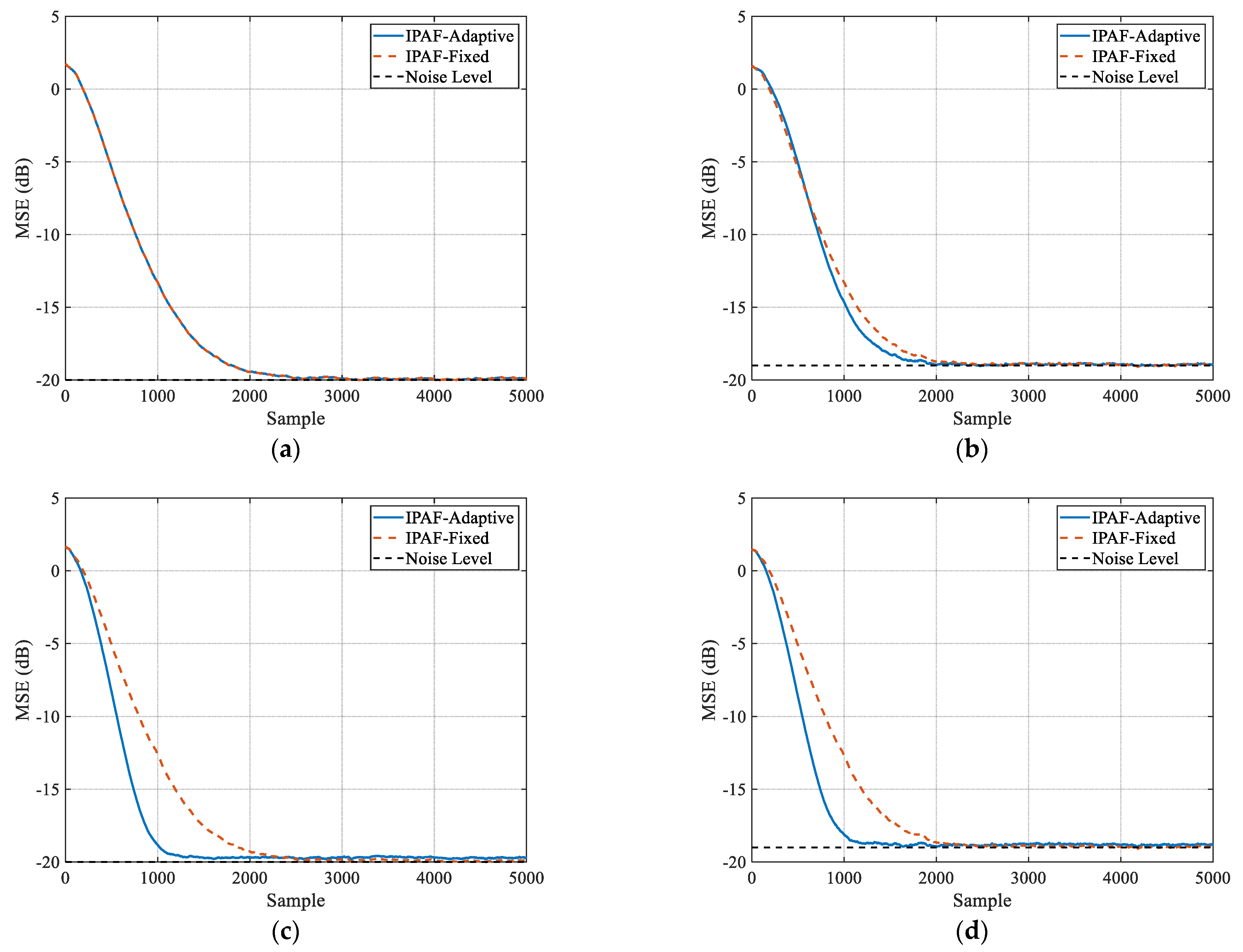
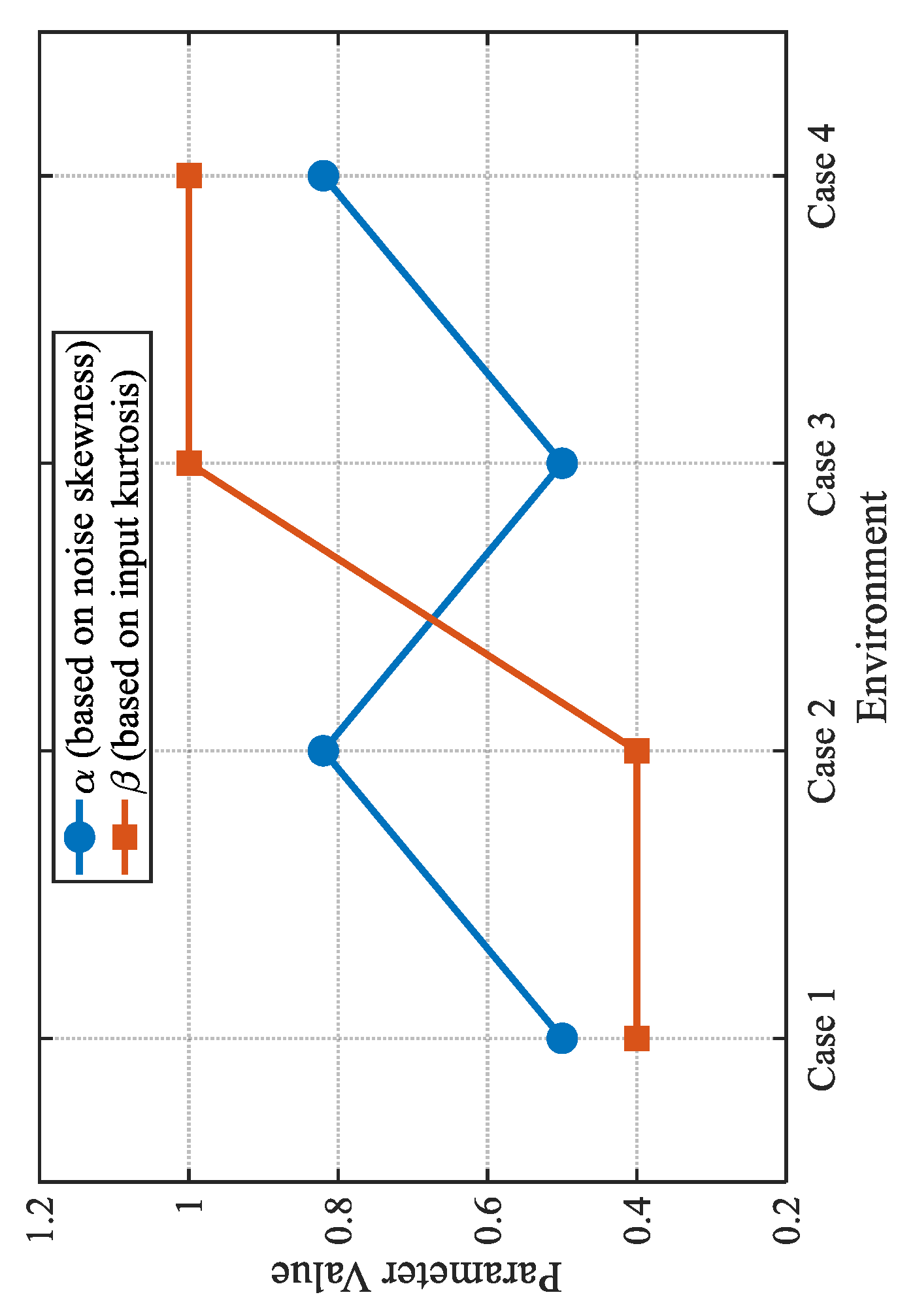
This section evaluates the effectiveness of the proposed information perception strategy in enhancing the performance of the IPAF algorithm by comparing its implementations with and without the strategy. Four experimental scenarios are considered: Gaussian input, non-Gaussian input with symmetric noise, and two configurations combining asymmetric noise. For the fixed-parameter version of the IPAF algorithm, the parameters are set as α = 0.5 and β = 0.3. The simulation results, presented in Figure 2, demonstrate that incorporating the information perception strategy not only improves the performance of the IPAF algorithm but also eliminates the need for manual parameter optimization. Figure 3 illustrates the trend of the α and β parameter values with the environment under the information-aware strategy.

4.2. Algorithm Performance Comparison

In this paper, an AF algorithm with an information perception strategy, referred to as the IPAF algorithm, is designed and proposed based on the concept of information perception.
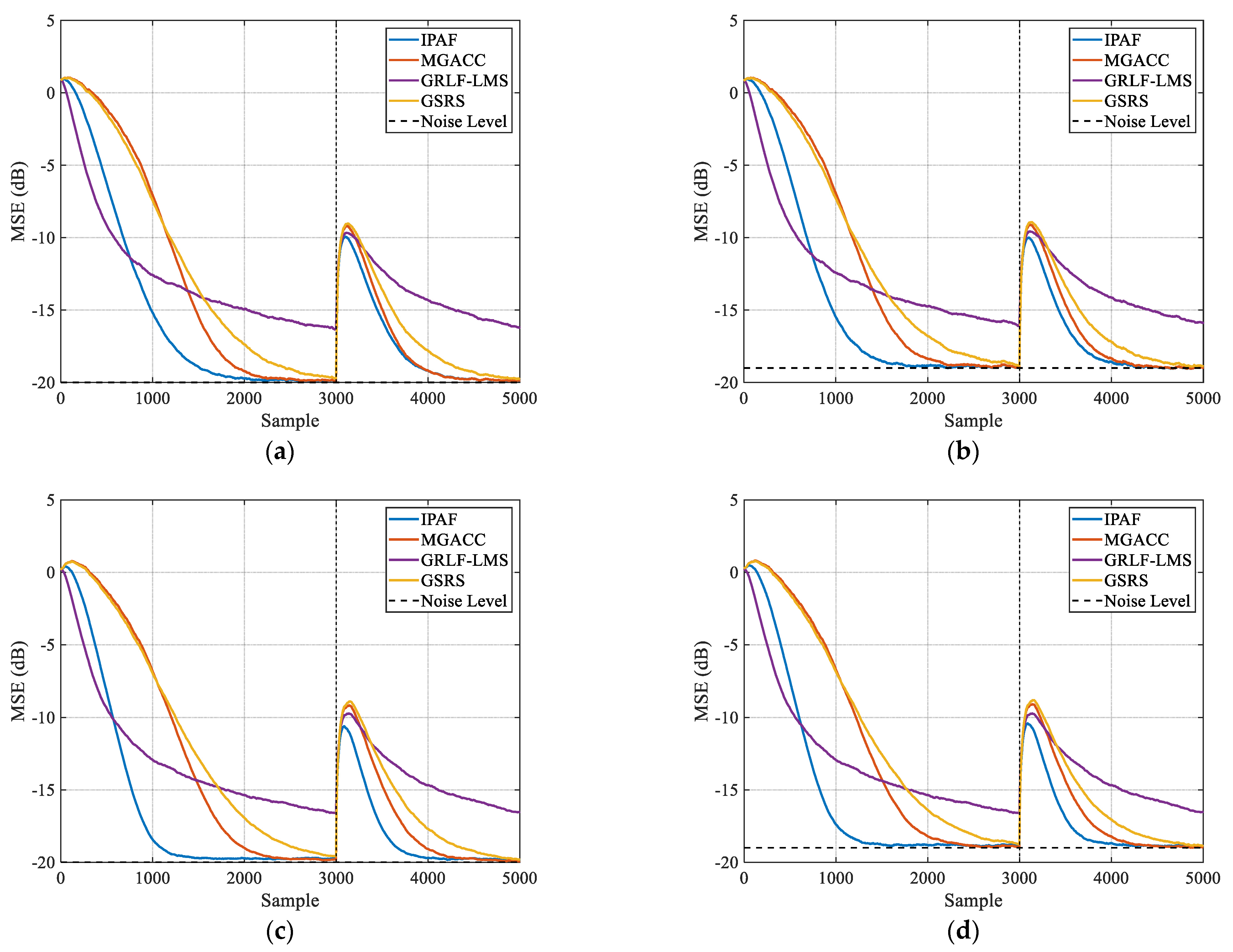
This section presents a comparative analysis of the convergence performance of the algorithms under four different environments. The validation is conducted through two simulation cases: Case 1, configured without systematic mutation, and Case 2, configured with systematic mutation. In the non-Gaussian setting, a heavy-tailed distribution is adopted to evaluate the algorithm’s performance under heavy-tailed conditions. In contrast, in the asymmetric noise setting, a right-skewed distribution is introduced to investigate the impact of biased noise on the algorithm’s robustness.

4.2.1. Case 1

Case 1 assesses the convergence performance of the IPAF algorithm in comparison to several algorithms known for their robustness in diverse environments. The results, depicted in Figure 4, demonstrate that the IPAF algorithm exhibits notably superior convergence compared to the other algorithms across four distinct environments. It reflects the ability to rapidly approach the vicinity of the target value while maintaining steady-state performance. Despite some degradation in performance across various scenarios, the IPAF algorithm consistently outperforms the alternatives.

4.2.2. Case 2

Case 2 verifies the robust performance of the IPAF algorithm and the comparison algorithm in various environments, including those with abrupt system changes. The experimental results, shown in Figure 5, indicate that the algorithm designed in this paper can still converge very quickly and exhibits better robustness performance after a sudden change in the system.

4.3. Daisy

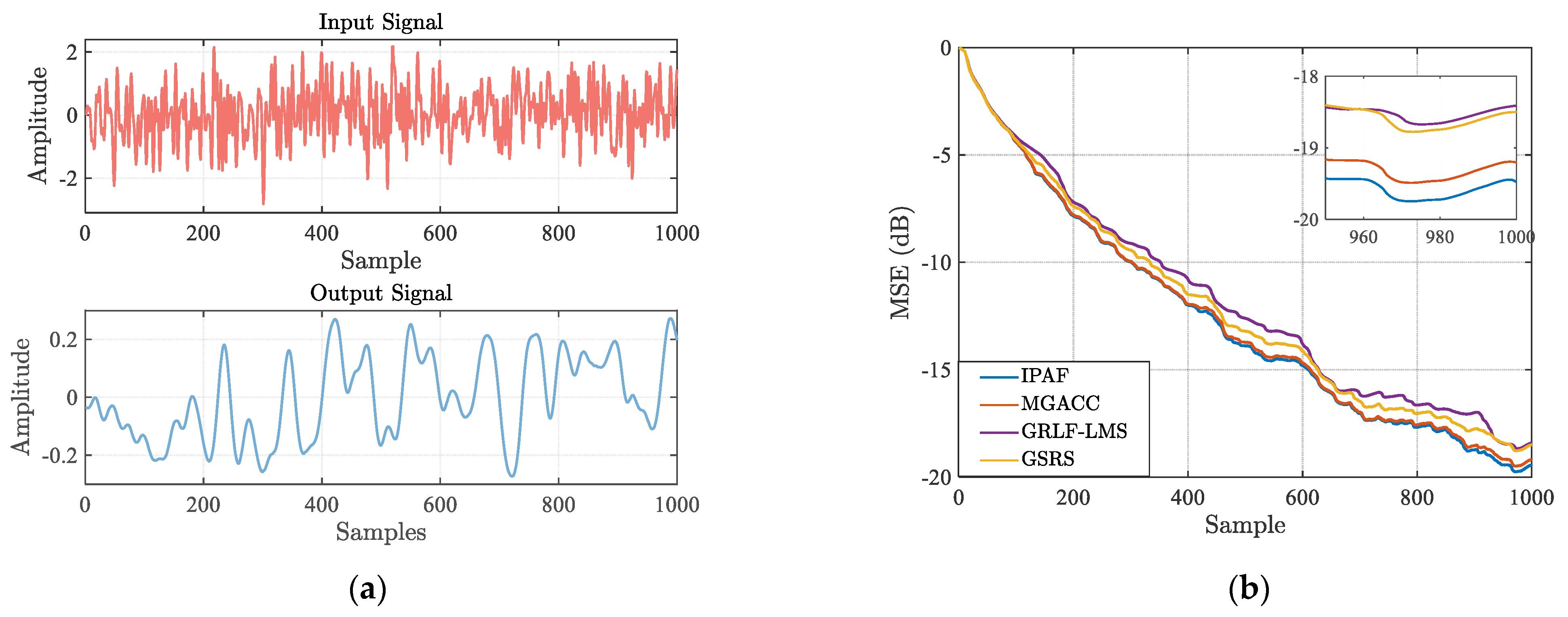
To evaluate the practical applicability of the proposed algorithm, two publicly available real datasets [35,36] are employed. The corresponding experimental results are presented in Figure 6 and Figure 7. Specifically, the data in Figure 6 are obtained from open experimental datasets, as shown in Figure 6a,b illustrate the comparative convergence performance of the algorithms across different datasets. In contrast, the data in Figure 7 are derived from actual engineering scenarios, as shown in Figure 7a, which depicts the relationship between input and output, and Figure 7b demonstrates the convergence performance of various algorithms. Overall, the experimental results confirm that the algorithm proposed in this study achieves superior convergence performance across different real datasets.

5. Conclusions

In this paper, an AF algorithm with an information perception strategy, referred to as the IPAF algorithm, is designed and proposed based on the concept of information perception. Through detailed theoretical derivations, the convergence interval and the minimum mean square deviation of the algorithm are established, and its computational complexity is systematically analyzed and compared. The results demonstrate that the proposed algorithm achieves superior convergence and steady-state performance while maintaining low computational complexity. Furthermore, extensive experiments verify that incorporating the information perception strategy significantly enhances algorithmic performance. The algorithm consistently preserves its advantages under heavy-tailed and asymmetric noise conditions, and it also delivers outstanding results when applied to real datasets. Therefore, the IPAF algorithm designed in this study realizes information perception through the proposed strategy and is validated as a reliable solution with remarkable robustness across diverse experimental settings.
It is worth noting that this paper proposes a novel approach to information perception through AF algorithms that utilize generalized cost functions. Currently, the method is implemented under the assumption that both input signals and noise are known. Therefore, future research should address scenarios where input signals and noise are unknown, thereby achieving the objective of “real-time information perception”.

Author Contributions

S.Y.: Software, Formal Analysis, Writing—Original Draft. S.G.: Methodology, Software, Formal Analysis, Supervision, Writing—Review and Editing, Funding acquisition. Y.Z., Q.X. and C.Z.: Writing—Review and Editing. B.B.: Writing—Review and Editing, Funding acquisition. All authors have read and agreed to the published version of the manuscript.

Funding

This work is financially supported by the National Natural Science Foundation of China (8225041038), the Fundamental Research Funds for the Central Universities, Southwest Minzu University (ZYN2025259), the 2025 Open Fund Research at the key Laboratory of Electronic and Information Engineering (Southwest Minzu University), State Ethnic Affairs Commission (No: EIE202502), and the Innovative Research Project for Graduate Students at Southwest Minzu University (Project No. YCZD2025XXX).

Data Availability Statement

Two publicly archived datasets were analyzed or generated during the study. https://www.nonlinearbenchmark.org/benchmarks/wiener-hammerstein-process-noise (accessed on 12 October 2025), and “Database for the Identification of Systems (http://homes.esat.kuleuven.be/~smc/daisy/)” (accessed on 12 October 2025).

Conflicts of Interest

The authors declare no conflicts of interest.

References

  1. Balassa, B.E.; Nagy, N.G.; Gyurian, N. Perception and social acceptance of 5G technology for sustainability development. J. Clean. Prod. 2024, 467, 142964. [Google Scholar] [CrossRef]
  2. Bonci, A.; Cen Cheng, P.D.; Indri, M.; Nabissi, G.; Sibona, F. Human-robot perception in industrial environments: A survey. Sensors 2021, 21, 1571. [Google Scholar] [CrossRef] [PubMed]
  3. Zhang, J.; Li, Z.; Chen, Y.; Lu, W.; Yi, F.; Liu, M. Passive sensing using multiple types of communication signal waveforms for Internet of Everything. IEEE Internet Things J. 2024, 11, 29295–29307. [Google Scholar] [CrossRef]
  4. Xiao, F.; Zeng, J.; Li, Z.; Chen, C.; Guo, W.; Zhang, Y.; Zhu, L.; Qiu, W. Research on the construction of information perception technology methods and models for global strategic mineral resources. China Min. Mag. 2025, 34, 48–56. [Google Scholar] [CrossRef]
  5. He, J.; Wang, G.; Zhang, X.; Wang, H.; Peng, B. Maximum total generalized correntropy adaptive filtering for parameter estimation. Signal Process. 2023, 203, 108787. [Google Scholar] [CrossRef]
  6. Zhang, X.-D. Modern Signal Processing; Walter de Gruyter GmbH & Co KG: Berlin, Germany, 2022. [Google Scholar]
  7. Zhang, X.; Ding, F. Adaptive parameter estimation for a general dynamical system with unknown states. Int. J. Robust Nonlinear Control 2020, 30, 1351–1372. [Google Scholar] [CrossRef]
  8. Li, M.; Liu, X. Iterative identification methods for a class of bilinear systems by using the particle filtering technique. Int. J. Adapt. Control Signal Process. 2021, 35, 2056–2074. [Google Scholar] [CrossRef]
  9. Zhang, X.; Ding, F. Optimal adaptive filtering algorithm by using the fractional-order derivative. IEEE Signal Process. Lett. 2021, 29, 399–403. [Google Scholar] [CrossRef]
  10. Bradley, V.M. Learning Management System (LMS) use with online instruction. Int. J. Technol. Educ. 2021, 4, 68–92. [Google Scholar] [CrossRef]
  11. Alotaibi, N.S. The impact of AI and LMS integration on the future of higher education: Opportunities, challenges, and strategies for transformation. Sustainability 2024, 16, 10357. [Google Scholar] [CrossRef]
  12. Zhou, X.; Li, G.; Wang, Z.; Wang, G.; Zhang, H. Robust hybrid affine projection filtering algorithm under α-stable environment. Signal Process. 2023, 208, 108981. [Google Scholar] [CrossRef]
  13. Hou, Y.; Li, G.; Zhang, H.; Wang, G.; Zhang, H.; Chen, J. Affine projection algorithms based on sigmoid cost function. Signal Process. 2024, 219, 109397. [Google Scholar] [CrossRef]
  14. Paleologu, C.; Benesty, J.; Ciochină, S. Data-reuse recursive least-squares algorithms. IEEE Signal Process. Lett. 2022, 29, 752–756. [Google Scholar] [CrossRef]
  15. Gao, W.; Chen, J.; Richard, C. Theoretical analysis of the performance of the data-reuse RLS algorithm. IEEE Trans. Circuits Syst. II Express Briefs 2023, 71, 490–494. [Google Scholar] [CrossRef]
  16. Ling, Q.; Ikbal, M.A.; Kumar, P. Optimized LMS algorithm for system identification and noise cancellation. J. Intell. Syst. 2021, 30, 487–498. [Google Scholar] [CrossRef]
  17. Alharbi, A.; Aljojo, N.; Zainol, A.; Alshutayri, A.; Alharbi, B.; Aldhahri, E.; Khairullah, E.F.; Almandeel, S. Identification of critical factors affecting the students’ acceptance of Learning Management System (LMS) in Saudi Arabia. Int. J. Innov. 2021, 9, 353–388. [Google Scholar] [CrossRef]
  18. Zerguine, A.; Ahmad, J.; Moinuddin, M.; Al-Saggaf, U.M.; Zoubir, A.M. An efficient normalized LMS algorithm. Nonlinear Dyn. 2022, 110, 3561–3579. [Google Scholar] [CrossRef]
  19. Li, L.; Zhao, X. Variable step-size LMS algorithm based on hyperbolic tangent function. Circuits Syst. Signal Process. 2023, 42, 4415–4431. [Google Scholar] [CrossRef]
  20. Guan, S.; Biswal, B. Spline adaptive filtering algorithm based on different iterative gradients: Performance analysis and comparison. J. Autom. Intell. 2023, 2, 1–13. [Google Scholar] [CrossRef]
  21. Le, D.C. Hierarchical learning-based cascaded adaptive filtering for nonlinear system identification. Digit. Signal Process. 2025, 160, 105031. [Google Scholar] [CrossRef]
  22. Xiang, S.; Zhao, C.; Gao, Z.; Yan, D. Low-Complexity Constrained Recursive Kernel Risk-Sensitive Loss Algorithm. Symmetry 2022, 14, 877. [Google Scholar] [CrossRef]
  23. Cai, B.; Wang, B.; Zhu, B.; Zhu, Y. An improved proportional normalization least mean p-power algorithm for adaptive filtering. Circuits Syst. Signal Process. 2023, 42, 6951–6965. [Google Scholar] [CrossRef]
  24. Wang, X.; Han, J. Affine projection algorithm based on least mean fourth algorithm for system identification. IEEE Access 2020, 8, 11930–11938. [Google Scholar] [CrossRef]
  25. Wang, S.; Wang, W.; Xiong, K.; Iu, H.H.; Tse, C.K. Logarithmic hyperbolic cosine adaptive filter and its performance analysis. IEEE Trans. Syst. Man Cybern. Syst. 2019, 51, 2512–2524. [Google Scholar] [CrossRef]
  26. Liang, T.; Li, Y.; Zakharov, Y.V.; Xue, W.; Qi, J. Constrained least lncosh adaptive filtering algorithm. Signal Process. 2021, 183, 108044. [Google Scholar] [CrossRef]
  27. Guan, S.; Cheng, Q.; Zhao, Y.; Biswal, B. Diffusion adaptive filtering algorithm based on the Fair cost function. Sci. Rep. 2021, 11, 19715. [Google Scholar] [CrossRef]
  28. Kumar, K.; Pandey, R.; Bora, S.S.; George, N.V. A robust family of algorithms for adaptive filtering based on the arctangent framework. IEEE Trans. Circuits Syst. II Express Briefs 2021, 69, 1967–1971. [Google Scholar] [CrossRef]
  29. Huang, F.; Zhang, J.; Zhang, S. A family of robust adaptive filtering algorithms based on sigmoid cost. Signal Process. 2018, 149, 179–192. [Google Scholar] [CrossRef]
  30. Abdelrhman, O.M.; Sen, L. Robust adaptive filtering algorithms based on the half–quadratic criterion. Signal Process. 2023, 202, 108775. [Google Scholar] [CrossRef]
  31. Abdelrhman, O.M.; Dou, Y.; Li, S. A generalized robust logarithmic family-based adaptive filtering algorithms. IEEE Trans. Circuits Syst. II Express Briefs 2023, 70, 3199–3203. [Google Scholar] [CrossRef]
  32. Patel, V.; Bhattacharjee, S.S.; Christensen, M.G. Generalized soft-root-sign based robust sparsity-aware adaptive filters. IEEE Signal Process. Lett. 2023, 30, 200–204. [Google Scholar] [CrossRef]
  33. Tang, J.; Li, Y.; Hou, Z.; Fu, S.; Tian, Y. Robust two-stage instance-level cost-sensitive learning method for class imbalance problem. Knowl. Based Syst. 2024, 300, 112143. [Google Scholar] [CrossRef]
  34. Wang, W.; Zhao, H.; Zeng, X. Geometric algebra correntropy: Definition and application to robust adaptive filtering. IEEE Trans. Circuits Syst. II Express Briefs 2019, 67, 1164–1168. [Google Scholar] [CrossRef]
  35. Schoukens, M.; Noël, J.P. Wiener-Hammerstein Process Noise System. Available online: https://www.nonlinearbenchmark.org/benchmarks/wiener-hammerstein-process-noise (accessed on 12 October 2025).
  36. Database for the Identification of Systems. Available online: http://homes.esat.kuleuven.be/~smc/daisy/ (accessed on 12 October 2025).
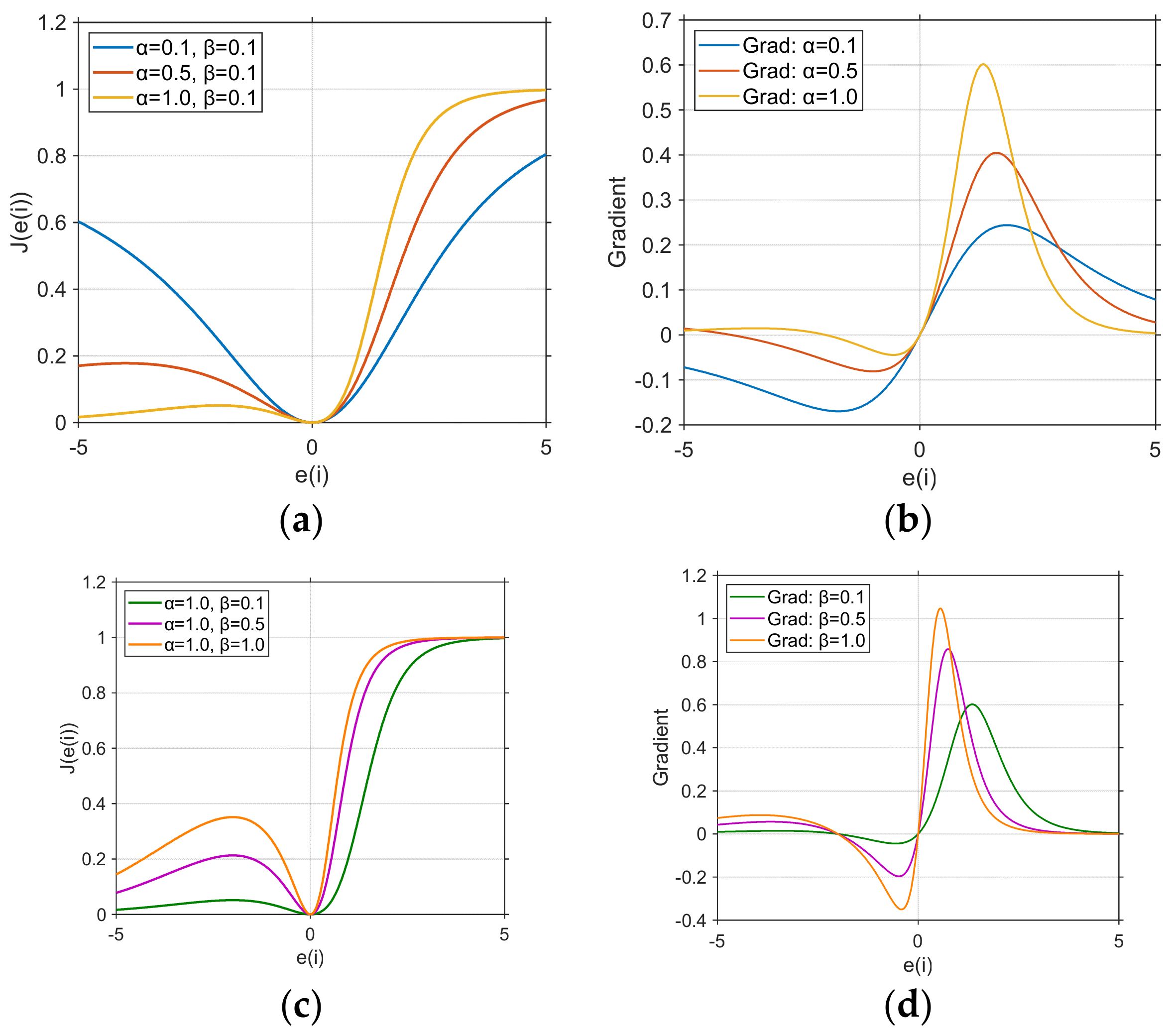
Figure 1. Cost function images over gradient images for different parameter values (a,b) α = 0.1, α = 0.5, α = 1.0; (c,d) β = 0.1, β = 0.5, β = 1.0.
Mathematics 13 03294 g001
Figure 2. Effect of adaptive strategy on algorithm convergence performance. (a) Gaussian input + symmetric noise, (b) Gaussian input + asymmetric noise, (c) non-Gaussian input + symmetric noise, and (d) non-Gaussian input + asymmetric noise. The step size is uniformly set to μ = 0.005.
Mathematics 13 03294 g002
Figure 3. Trends in α and β.
Mathematics 13 03294 g003
Figure 4. Comparison of convergence performance of different algorithms. (a) Gaussian input + symmetric noise, (b) Gaussian input + asymmetric noise, (c) non-Gaussian input + symmetric noise, and (d) non-Gaussian input + asymmetric noise. The step size is uniformly set to μ = 0.005.
Mathematics 13 03294 g004
Figure 5. Comparison of convergence performance of different algorithms after encountering abrupt system changes. (a) Gaussian input + symmetric noise, (b) Gaussian input + asymmetric noise, (c) non-Gaussian input + symmetric noise, and (d) non-Gaussian input + asymmetric noise. The step size is uniformly set to μ = 0.005.
Mathematics 13 03294 g005
Figure 6. Real datasets. (a) Learning rate of different algorithms on the data from WH_TestDataset.csv. (b) Learning rate of different algorithms on the data from WH_EstimationExample.csv. The step size is uniformly set to μ = 0.05.
Mathematics 13 03294 g006
Figure 7. Real datasets. (a) Input and output variables of data from a flexible robot arm (No. 96-009). (b) Learning rate of different algorithms on an industrial dataset. The step size is uniformly set to μ = 0.02.
Mathematics 13 03294 g007
Table 1. Computational complexity of algorithms.
Algorithm+×÷exp (·)
IPAF2L + 22L + 923
MGACC [34]2L2L + 312
GRLF-LMS [31]2L + 12L + 312
GSRS [32]2L + 22L + 725
Disclaimer/Publisher’s Note: The statements, opinions and data contained in all publications are solely those of the individual author(s) and contributor(s) and not of MDPI and/or the editor(s). MDPI and/or the editor(s) disclaim responsibility for any injury to people or property resulting from any ideas, methods, instructions or products referred to in the content.