Abstract
Cassava is the sixth most important food crop worldwide and the third most important source of calories in the tropics. More than 800 million people depend on this plant’s tubers and sometimes leaves. To protect cassava crops and the livelihoods depending on them, we developed a stochastic fractional delayed model based on stochastic fractional delay differential equations (SFDDEs) to analyze the dynamics of cassava mosaic disease, focusing on two equilibrium states, the state of being absent from cassava mosaic disease and the state of being present with cassava mosaic disease. The basic reproduction number and sensitivity of parameters were estimated to characterize the level beyond which cassava mosaic disease prevails or declines in the plants. We analyzed the stability locally and globally to determine the environment that would ensure extinction and its persistence. To support the theoretical analysis, as well as the reliable results of the model, the present study used a nonstandard finite difference (NSFD) method. This numerical method not only improves the model’s accuracy but also guarantees that cassava mosaic probabilities are positive and bounded, which is essential for the accurate modeling of the cassava mosaic processes. The NSFD method was applied in all the scenarios, and it was determined that it yields adequate performance in modeling cassava mosaic disease. The ideas of the model are crucial for exploring key variables, which affect the scale of cassava mosaic and the moments of intervention. The present work is useful for discerning the mechanism of cassava mosaic disease as it presents a solid mathematical model capable of determining the stage of cassava mosaic disease.
Keywords:
cassava mosaic disease; stochastic fractional delay differential equations; existence and uniqueness; stability results; extinction and persistence; NSFD; results MSC:
65M06; 65M12; 35K15; 35K55; 35K57
1. Introduction
In [1], the authors established and tested a detailed mathematical model, designed to investigate the modes of transmission of cassava mosaic disease (CMD) in cassava plants. As such, this offers important knowledge on the mode of transmission and determinants of the disease in agricultural systems. In [2], the authors established a fractional model for the dynamics of cassava mosaic disease (CMD) with Caputo Fabrizio (CF) fractional derivative. This approach was meant to reduce the infection rates in cassava plants in a bid to capture real-life scenarios better within disease distribution. In [3], the authors proposed a model for describing the transmission dynamics of cassava mosaic disease (CMD) with an ordinary differential equations (ODEs) system. It also provides a control strategy of performing the best method in enhancing the management and reduction of the spread of the disease, including cutting off the affected cassava plants and use of insecticides. In [4], the authors included the designing, coding, and testing of an optimality system for managing CMD, in a simulation. This was instigated through the casing of the infected cassava and non-cassava host plants practices, as well as the use of insecticides. In [5], the authors explored and tested the efficiency of deep learning approaches for the identification of cassava mosaic disease (CMD) in cassava and other diseases in the tomato plant leaves. To bring about better early disease detection and better crop handling through self-learning, upcoming models of machine learning (ML) are utilized. In [6], the authors provided a dependable decision-making tool in the promotion of healthy seed systems, especially in addressing cassava mosaic disease. It involved the management of seeds and their distribution, hence promoting sustainable agriculture and improving the resistance of the cassava crop to the disease. In [7], the authors employed a computational model that instantiates both landscape and field simulations of cassava brown streak disease (CBSD). In [8], the authors studied the gene expression patterns of a cassava cultivar with resistance to given stress factors in comparison with a susceptible cassava cultivar. In [9], the authors studied cassava brown streak disease and its consequences. In [10], the authors developed and refined a real-time quantitative diagnostic protocol for detecting cassava common mosaic virus (CCMV); this would likely offer a more accurate and sensitive alternative compared to all other molecular techniques. Optimized conditions for virus detection would enhance the efficiency of detecting viruses and potentially lead to better management of cassava crop health. In [11], the authors examined and forecasted both present and future situations concerning the spread and impact of cassava brown streak disease and the Benicia Tabaco species complex on cassava crops. In [12], the authors conducted a study in the five farming regions of Togo to determine the distribution and location of the East African cassava mosaic virus (EACMV) and the East African cassava mosaic Cameroon virus (EACMCMV). In [13], the authors proposed a system that is one of pre-trained models based on neural networks and deep learning. Designed to manage unclear data well, this system will offer a strong solution regarding the accurate identification of diseases. Advanced AI methods are expected to improve diagnostic accuracy and the efficiency of the process of disease detection. In [14], the authors focused on how the cassava brown streak disease is transmitted through cassava plants by considering genetic differences. They established better sources of resistance against the cassava brown streak disease. In [15], the authors created a very detailed model including how the virus, whitefly, and plant all interact—including changes in temperature. In [16], the authors demonstrated that target proteins help in the defense of the plant by activating genes that produce melatonin. In [17], the authors explored how the cassava common mosaic virus (CsCMV) influences the day-to-day carbon metabolism in cassava leaves, especially as far as the source–sink relationship is concerned. In [18], the authors compared various deep-learning techniques to find which ones can best classify cassava leaf diseases. It will be able to draw comparisons between different techniques and understand how one can improve disease detection on cassava plants through better farming. In [19], the authors determined the prevalence, frequency, and severity of cassava mosaic disease (CMD) and cassava brown streak disease (CBSD) in six western Kenya counties in the years 2022 and 2023. In [20], the authors developed a better classification of cassava leaf diseases. This model improves the quality of its features, mainly in the task of coarse label classification. Allen studied stochastic epidemic models including formulation, numerical simulation, and analysis [21]. Mamis et al. studied uncertainties in stochastic compartmental models [22].
The stochastic fractional delayed methodology has significant scientific benefits because it combines stochastic processes, fractional calculus, and temporal delays to mimic complex systems more precisely. This approach uses fractional derivatives to capture memory effects, which is important in fields like biology and economics since it accounts for past effects on current conditions. Temporal delays are incorporated to provide for a realistic depiction of the lag between cause and effect, while the stochastic component handles the inherent randomness in systems. Together, these elements enhance the models’ predictive power and robustness across multiple domains, rendering them more realistic representations of real-world dynamics.
The structure of the paper is as follows: Section 1 provides an overview and a detailed examination of cassava mosaic-like diseases that have been reported in the literature. Section 2 examines the construction of the stochastic fractional delayed cassava mosaic disease model; the resulting mathematical analysis; and the local and global levels of the model’s equilibria, reproduction number, and stability analysis. Section 3 shows a sensitivity analysis of the parameters involved in reproduction numbers. In Section 4, the model was examined using the NSFD approach. In Section 5, the positivity and boundedness of the NSFD are studied. In Section 6, the explicit focus is on numerical simulations of the model, including its discussion. Section 7 presents the conclusion of the study.
2. Model Formulation
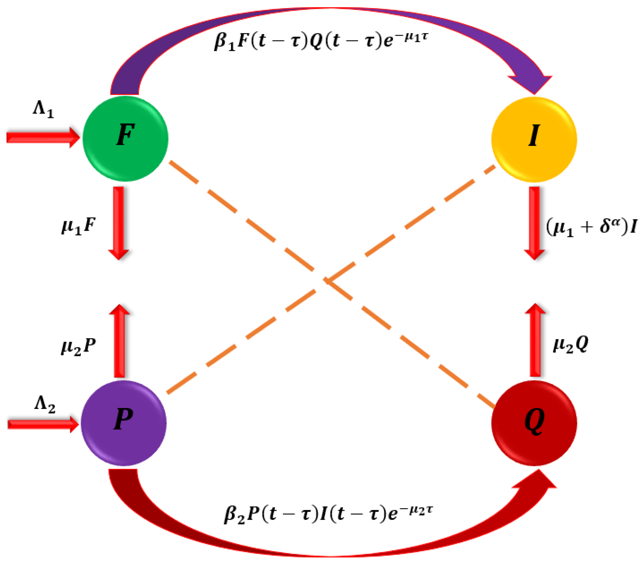
In this part, we enhance the model [1] by developing a mathematical model for cassava mosaic disease (CMD) transmission dynamics. The host population is made up of cassava plants, further separated into two subpopulations: the susceptible group and the infected group . The total number of cassava plants is determined by the formula . The population of whiteflies and the disease vectors are divided into sub-populations that are susceptible and infected , with the overall population of whiteflies determined by . Only diseased cassava may cause the vulnerable whitefly to become infected, and once it does, it never fully recovers. On the other hand, only infected whiteflies may infect vulnerable cassava plants, and once infected, the illness never goes away. The model accounts for susceptible whitefly recruitment at a rate of and the transformation of susceptible whiteflies to infected whiteflies at a rate of after connecting infected cassava plants. After being exposed to infected whiteflies, susceptible cassava plants are replanted at a rate of and change to infected cassava plants at a rate of . The model also takes into consideration the natural mortality rates of whiteflies and cassava plants , as well as the CMD mortality rate from the stated infected (see Figure 1).
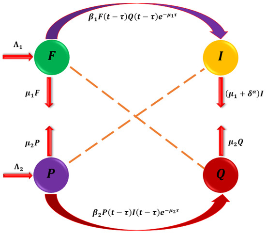
Figure 1.
The interactions that occur between susceptible populations and infections.
Cassava mosaic disease (CMD) is a complex illness that has complex dynamics. The basic structure for the investigations is the deterministic model [1], whereby the first-order temporal derivatives are substituted by fractional Caputo derivatives of order . We believe that such an adjustment provides a more appropriate picture of the diffusion of cassava mosaic disease. These equations describe how the infection spreads and changes throughout the population of cassava plants, impacting disease development, transmission, and possible management approaches. The set of differential equations that follows described the model [23].
The nonnegative (initial) conditions for the system (1)–(4) are
This strategy indicates how the random disturbances in the system can be represented by the stochastic fluctuations . Let be Brownian motion, a continuous stochastic process for time . The parameter acts as a time delay to the system provided that , and also so that the effect of the delayed feedback is visible only after a time interval.
Preliminaries: The following are the fundamental preliminary definitions that explain the fractional derivative in the context of Caputo:
Definition 1.
For a function
, the Caputo fractional derivative of order
is
Definition 2.
For the function
, the expression describes the equivalent fractional integral with order .
where is the gamma function displayed.
2.1. Existence and Uniqueness of the Stochastic Fractional Delayed Model
This section of the paper establishes the stochastic fractional delayed model’s existence and uniqueness. Apply the fractional integral in this case, assuming under the system (1)–(4) starting condition [24,25].
The functions defined under the integral in system (5)–(8) are
Furthermore, it is assumed that exist as positive constants and that are non-negative limiting functions.
Such that
Theorem 1.
The function
for
fulfills the Lipshitz requirement and are contraction mappings by assuming
, if the condition
is true.
Proof.
First, we consider the function . Examine the subsequent and :
In this instance, . Lipshitz’s condition is satisfied. This method may also be used to meet the Lipschitz criteria for . Additionally, if , then the functions are contractions. Furthermore, there is constant writing in system (9)–(12).
The two terms’ variation is represented by the following in (14)–(17):
Therefore, we have
Let
□
The remaining equations in system (19)–(21) might be solved using the same method to obtain
as required.
Theorem 2.
Show that
The system (18)–(21) has a specified uniform function.
if there is a
such that
. Assuming
, the model system has at least one solution if
for
.
Proof.
Since each kernel for , satisfies the Lipschitz condition and the functions are bounded, the following relations may be determined:
in the system (30)–(33) figure, it is demonstrated that the function given in (22)–(25) exists and is consistent. It is necessary to show that converge to the system of solutions of (1)–(4) to prove (ii). To do this, we define the remaining terms after changes as . Thus,
By using the Lipschitz condition and the triangle inequality, we determine that
When the process in (38) is repeated, we obtain
Next, at , one acquires
Assuming as the limit.
By applying the hypothesis , we have from (41) yield.
□
By using the same process as for n→ ∞, we obtain
As a result, there must be only one solution, as desired.
Theorem 3.
If
for the assumption
, then demonstrate the uniqueness of the system (1)–(4).
Proof.
Consider that another collection of solutions to (1)–(4) is represented by the sets .
If the terms in (46) are rearranged, one obtains
By applying the hypothesis , we have from (47) yield.
It follows from this because . Applying the identical process to every solution for , we arrive at
hence proved. □
Theorem 4.
For the initial conditions with assumption
, prove that the fractional delayed model (1)–(4) has a positive solution in
.
Proof.
The feasible situation must be non-negative across the system to be considered under the initial condition. We obtain
□
Hence, the fractional delayed model (1)–(4) has a positive solution, when the initial condition falls inside the feasible region.
Theorem 5.
The system (1)–(4) in the feasible region
; (where
and
are plants and whiteflies population) at any given time
. The initial condition is bounded with the assumption that
.
Proof.
The total sum of plant population can be written as
After resolving the inequality above, we obtain
Using Grown’s inequality [25],
Similarly, the total sum of the whitefly population can be written as
After resolving the inequality above, we obtain
Using Grown’s inequality,
□
Therefore, the epidemiologically feasible region for the propagation of cassava mosaic disease is provided by (52)–(53).
The fractional delayed model (1)–(4) is both positively invariant and realistic from an epidemiological point of view concerning the transmission of the cassava mosaic disease (54).
Hence, the system (1)–(4) is bounded under the initial conditions.
2.2. Model Equilibria and Reproduction Number
In this part, we examine the different states of the fractional delayed model with the propagation of cassava mosaic disease dynamics. It allows us through the analysis of the system behavior to understand how the system behaves at the free and present state of the cassava mosaic equilibrium. It also provided information on how the fractional order, delays, and stochastic parameters behave and control the transmission of mosaic disease using different numerical techniques. Therefore,
In epidemiology, the basic reproduction number is an important parameter. This suggests whether or not the disease is prevalent in the general population. If the value of it is less than, the disease is not spreading in the population; otherwise, the disease is present in the population. For the evaluation of the reproduction number using the next-generation method, as a consequence, becomes the transmission matrix and the transition matrix.
The largest eigenvalue or spectral radius of , at the cassava mosaic-free equilibrium, is as follows:
Definition 3.
The infected group will be extinct in the system (1)–(4), if
,
.
Lemma 1.
(Gray et al. [26]). If < 1 and
, then the infected individuals of the system (1)–(4) exponentially tend towards zero.
Proof.
Let us consider the initial data and that the system (1)–(4) admits the solution as , with as the randomness, if it satisfies the stochastic differential equation:
By using the lemma with , we have
Notice that with .
If
If , then
, when , we get , , as desired. Thus,
□
Theorem 6.
Assuming
, the cassava mosaic-free equilibrium (55) is locally asymptotically stable for
if
and
.
Proof.
By linearizing the model (1)–(4) about (55), a dimensional Jacobian matrix with negative real components and eigenvalues is obtained.
□
As a result, the cassava mosaic-free equilibrium of the provided model (1)–(4) is locally asymptotically stable if . If , then (55) is unstable in the local sense.
Theorem 7.
Assuming
, the model (1)–(4) is globally asymptotically stable (GAS) at the cassava mosaic-free equilibrium,
if
.
Proof.
Define the Lyapunov function as
This implies that if and if . Therefore, is globally asymptotically stable. □
Theorem 8.
Assuming
, the cassava mosaic-present equilibrium (56) is locally asymptotically stable for
if
.
Proof.
The model (1)–(4) is linearized around (56) to obtain a dimensional Jacobian matrix with negative real components and eigenvalues. The fourth-order polynomial follows as
Here,
Which is the fourth-order polynomial where the coefficients of the polynomial and are positive with . So, by the Routh–Hurwitz criterion for a fourth-degree polynomial, the coefficient of the characteristic equation is positive with the constraint . Hence, the cassava mosaic-present equilibrium of the given system (1)–(4) is stable in the local sense. Or else, if then the Routh–Hurwitz condition for stability is violated. Thus, (56) is unstable in the local sense. □
Theorem 9.
Assuming
, the model (1)–(4) is globally asymptotically stable (GAS) at the cassava mosaic-present equilibrium,
if
.
Proof.
Define the Lyapunov function as
Given positive constants , we can express the following equation:
If we choose ,
, for and if and only if . Hence, by Lasalle’s invariance principle, is globally asymptotical stable. □
3. Sensitivity Analysis
In this section, we examine the behavior of model parameters concerning reproduction number . We examined the transmission and spread of disease with the sensitive analysis of the model. The formalized sensitivity index of a variable , that depends differentiable on a parameter is
In spatial terms, determine the sensitive indices of parameters concerning the reproduction number .
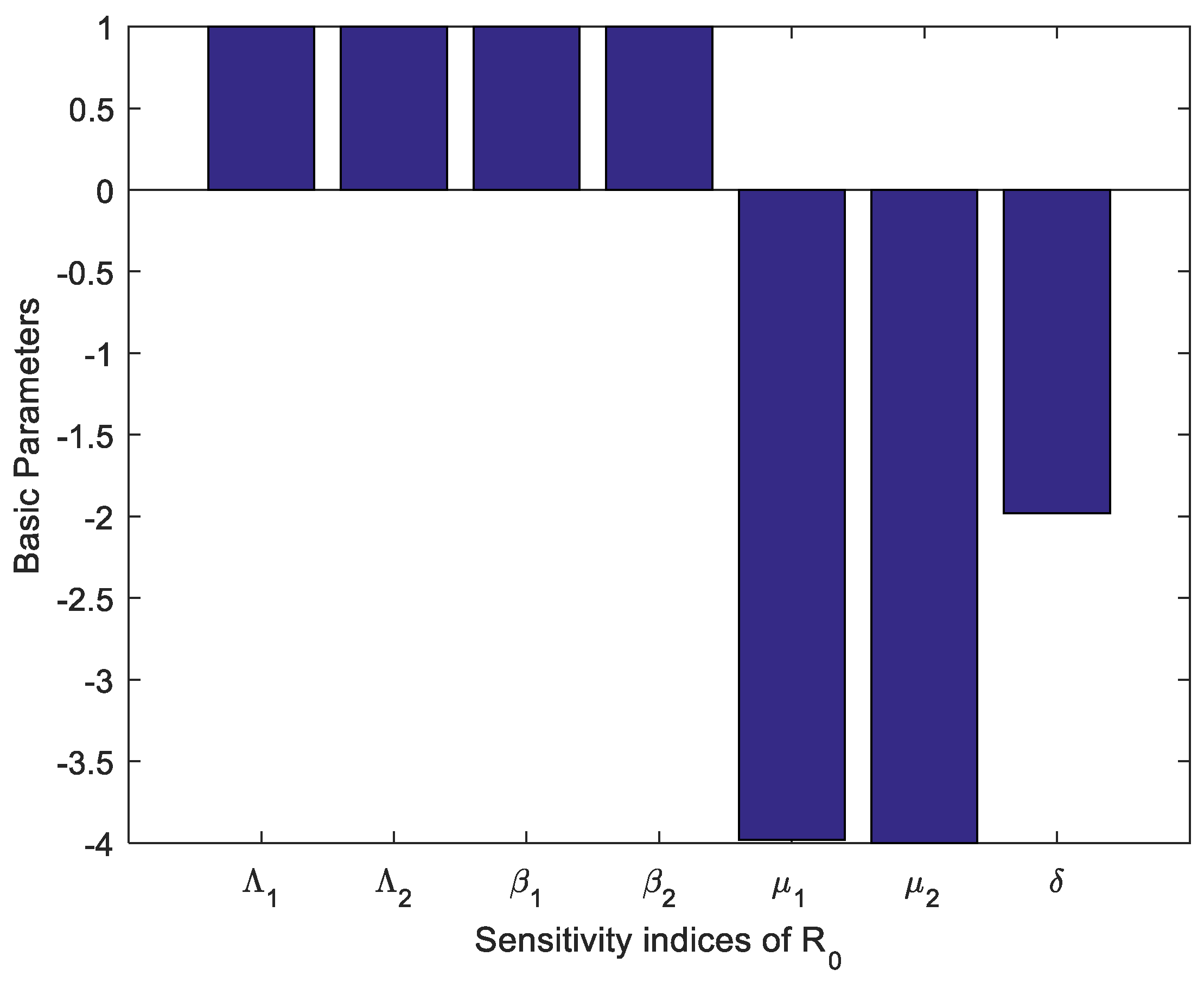
Table 1 and Table 2 provide the values of the sensitivity indicators together with the uncertainty indicators. All the parameters have positive sensitivity values. This means that the parameters have raised the value of and it becomes possible to make it high, hence making the system out of control. These parameters could represent transmission rates or factors that enhance the spread of the condition. The parameters associated with negative sensitivity values suggest that a higher value of these parameters results in a lower . These parameters probably measure recovery rates, death rates, or removal rates that decrease the persistence or spread of the condition. For instance, if , the model also illustrates that such parameters’ increase would imply a remarkably reduced reproduction number, which underlines the importance of recovery or intervention mechanisms. Figure 2 shows how different parameters affect . When increased, the parameters with negative sensitivity like decrease , and therefore the spread of the disease can be minimized if either recovery improves or transmission is lessened. Conversely, those factors that lead to higher values of sensitivity parameters are indicative of factors that raise the value of .

Table 1.
Parameters sensitivity signs.
Table 2.
Parameters’ sensitivity values.

Figure 2.
Sensitivity indices of reproduction number .
4. NSFD Method
This section presents a nonstandard finite difference method (NSFD) for the stochastic fractional delayed model (1)–(4) that underlies it. Another instance of the stochastic fractional delayed system is provided, and throughout, ∆t represents the temporal step-size.
NSFD rules, making the discrete model as
5. Properties
Theorem 10.
(Positivity). The deterministic form of system (62)–(65) preserves the non-negativity of the solution [27].
Proof.
All the equations in the system (62)–(65) contain no negative term. So, if the initial conditions are non-negative, then the numerical solutions remain non-negative, as desired. □
Theorem 11.
(Boundedness). Suppose that the initial data of (62)–(65) are non-negative. Then, there exists a constant
, such that
, for each
.
Proof.
By adding and rearranging the equations of the numerical model (62)–(65), we readily check that
The proof is established using mathematical induction, letting be the right end of this chain of identities and inequalities. □
Next, we examine the stability of the NSFD system (62)–(65).
Definition 4.
(Arenas et al. [28]). The discrete system (62)–(65) is asymptotically stable if there exists constants and
with the property that
as
.
Theorem 12.
Under the hypotheses of Theorem 10, the system (62)–(65) is asymptotically stable.
Proof.
The conclusion of this result is a direct consequence of Theorem 10. □
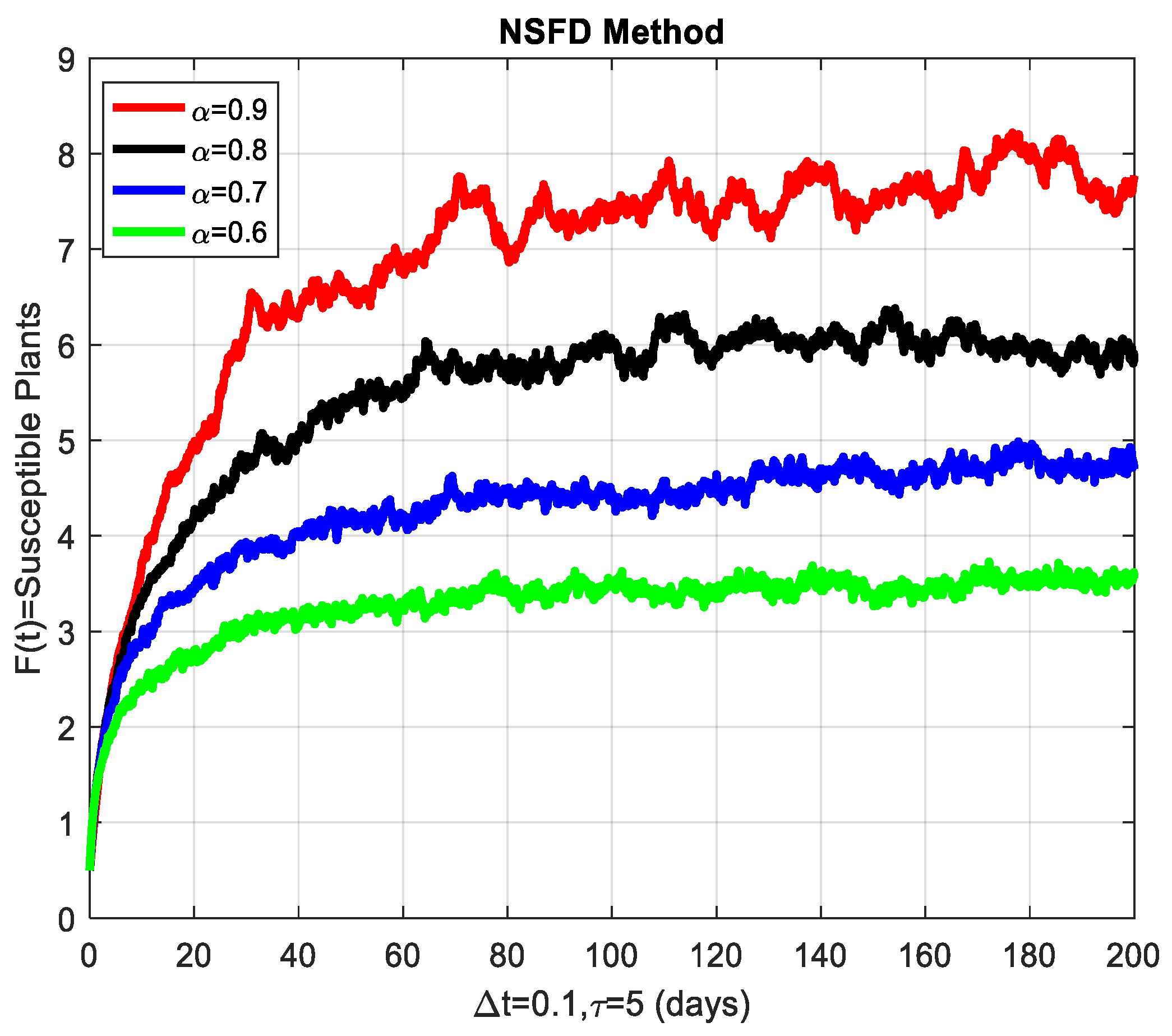
Before closing this section, we provide some numerical simulations for the stochastic fractional-order epidemic model (1)–(4). To that end, we fix the model parameters as given by Table 3 (see [1]). To start with, Figure 3 depicts the convergence behavior of each compartment of the model at the cassava mosaic-present equilibrium . The behavior of the graphs is investigated for various values of . Each graph adopts a random path to reach the cassava mosaic-present equilibrium at the temporal step-size . We conclude from this that the generalized NSFD method illustrates the actual behavior of the disease dynamics.
Table 3.
Values of parameters.
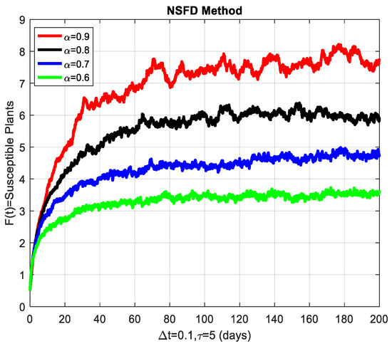
Figure 3.
The susceptible plants are shown graphically for different values of the fractional order α.
6. Numerical Simulations
The simulation parameter is explained in this section. The primary features of the simulated graphs were examined using the set of parametric variables given in Table 3. Furthermore, these graphs were created at the time when the disease is broadly exposed in the plant population and finally achieved a stable, present form. Appropriate values of α were selected at the current equilibrium to examine the dynamics of the disease.
Discussion
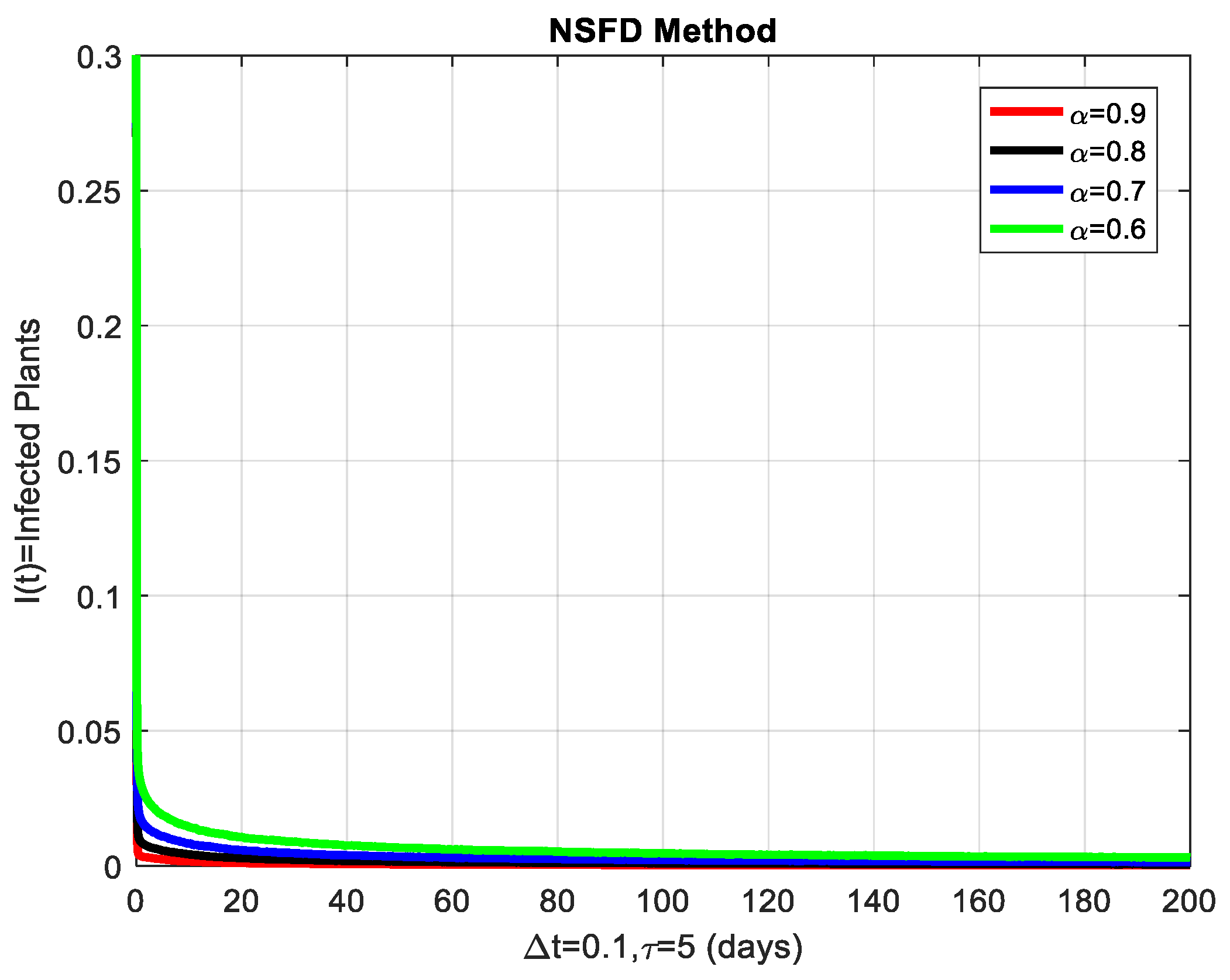
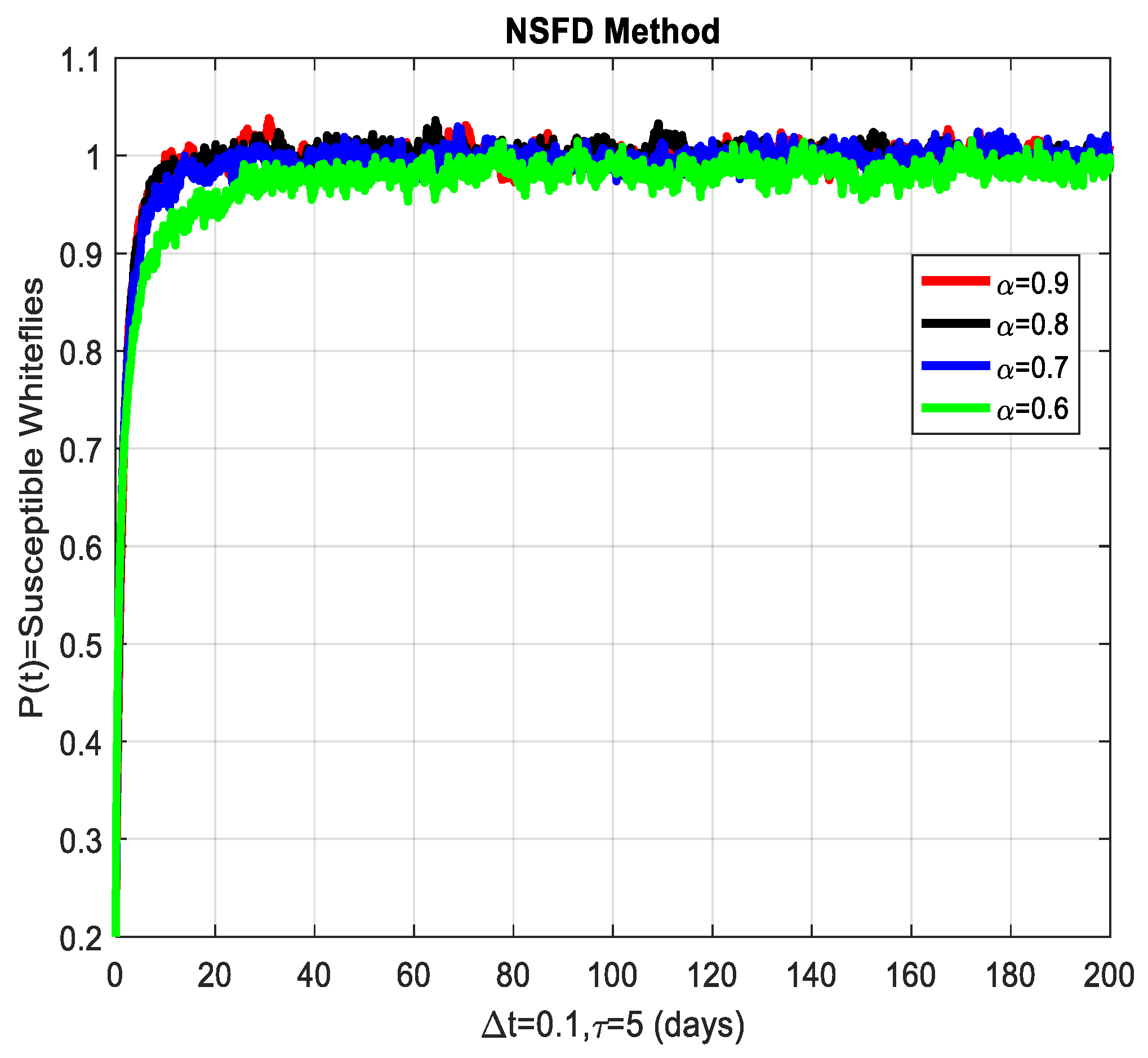
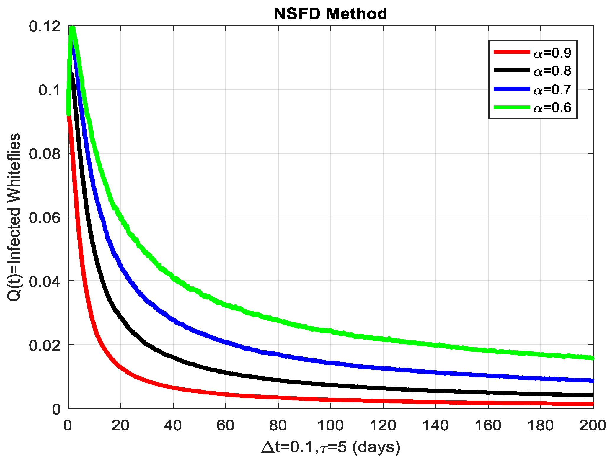
This section covers the discussion of graphical representations of the behavior of susceptible and infected plants and whiteflies for different values of the fractional order with time delay . In Figure 3, susceptible plants over time using various fractional order values are plotted. A higher value corresponds to a slower decrease in susceptible plants, indicating that as decreases, the rate at which plants become infected increases. This means that the fractional order influences the changes in disease transmission dynamics because the higher susceptible rate decreases with increasing . The infected plants over time are illustrated in Figure 4 for the various values. Thus, the rate of anticipating infections increases rapidly when is small, which is when the current number of infected plants is growing at a higher pace. This means that a low value for implies a higher rate of spread of disease within the plant population, proving that is a key player in invasion props. In Figure 5, for the plants, the behaviors of susceptible whiteflies is presented for different values. As the fractional order decreased, the rate of the whiteflies becoming infected was higher, so the decline of the susceptible whiteflies was much faster. Further evidence is provided therefore by the fact that lower values increase the rate at which the disease spreads within the whiteflies. In the infected whiteflies (Figure 6), the infection dynamics among the whitefly population are presented concerning different values. As with the plants, a low value causes an exponential growth of the infected whiteflies more easily. This brings the favorable use of in studying and estimating the course of the disease, for example among vectors such as the whitefly, which contributes towards the spread of plant diseases.

Figure 4.
The infected plants are shown graphically for different values of the fractional order α.
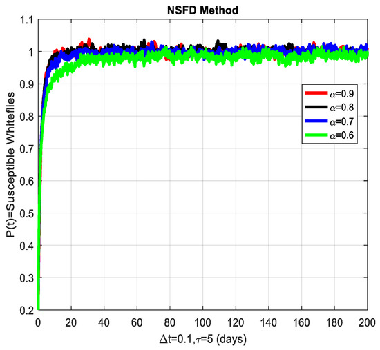
Figure 5.
The susceptible whiteflies’ graphical behavior for different values of fractional order α.
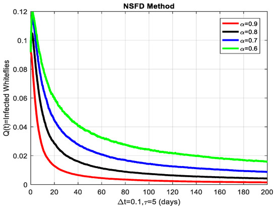
Figure 6.
The infected whiteflies showing graphical behavior for different values of fractional order α.
7. Conclusions
The examination of the probabilistic model that incorporates the parameter of delayed cassava mosaic disease is essential in studying the process of cassava mosaic disease spreading among individuals. The presented model combines methods based on mathematical analysis and numerical simulations, which are sufficient for capturing the system’s response under different conditions. The use of the stochastic NSFD scheme for numerical solutions guarantees features such as positive and bounded solutions, which are important in any compartmental model, particularly in the context of propagation of disease. The model successfully identifies two equilibrium states, the cassava mosaic-free equilibrium and the cassava mosaic-present equilibrium. From graphical illustrations, one can identify the circumstances under which the present equilibrium, signifying continuous cassava mosaic disease, is physically possible to maintain. Simultaneously, the model shows that the cassava mosaic-free state is achievable with the right types of intervention strategies. Quantitative stability analysis indicates that the basic reproduction number influences the stability of the system. When , the only stable equilibrium is cassava mosaic-free, meaning that cassava mosaic disease can be eradicated if the right conditions are met. When , the present state of equilibrium is maintained, implying that although cassava mosaic disease is present, it can be managed. The model also incorporates the frequency, duration, and extent of delay tactics in the spread of cassava mosaic behaviors. Notably, delayed interventions may lead to lower transmission rates, but strict and timely intervention measures can prevent and consequently reduce its spread. This highlights the importance of adopting early intervention systems to prevent cassava mosaic disease. The extension of guidelines, similar to health SOPs, into this cassava mosaic model suggests that strictly following such guidelines could help minimize the level of cassava mosaic disease. Therefore, this stochastic fractional delayed cassava mosaic model can be useful for analyzing and modeling the effects of cassava mosaic disease in different populations. By analyzing delay strategies, distinct conclusions can be drawn regarding the formulation of valid public policies and prevention measures. Future studies can look at including spatial and climate factors to improve understanding of how cassava mosaic disease spreads.
Author Contributions
Conceptualization, A.R.; Methodology, F.M.; Software, A.R. and M.M.; Validation, F.M.; Formal analysis, A.R.; Investigation, U.S.; Resources, U.S. and M.M.; Data curation, F.M., A.R. and M.M.; Writing—original draft, A.R. and U.S.; Writing—review & editing, A.R. and U.S.; Visualization, M.M.; Supervision, F.M.; Project administration, F.M.; Funding acquisition, F.M. All authors have read and agreed to the published version of the manuscript.
Funding
This research was partially supported by the Fundação para a Ciência e Tecnologia, FCT, under the project https://doi.org/10.54499/UIDB/04674/2020.
Data Availability Statement
The datasets analyzed during the current study are available from the corresponding author upon reasonable request.
Conflicts of Interest
The authors affirm they have no conflicts of interest to disclose concerning the current study.
References
- Holt, J.; Jeger, M.J.; Thresh, J.M.; Otim-Nape, G.W. An epidemilogical model incorporating vector population dynamics applied to african cassava mosaic virus disease. J. Appl. Ecol. 2024, 34, 793–806. [Google Scholar] [CrossRef]
- Abdullah, T.Q.; Huang, G.; Al-Sadi, W.; Aboelmagd, Y.; Mobarak, W. Fractional Dynamics of Cassava Mosaic Disease Model with Recovery Rate Using New Proposed Numerical Scheme. Mathematics 2024, 12, 2386. [Google Scholar] [CrossRef]
- Sangsawang, S.; Khan, A.; Pongsumpun, P. Sensitivity analysis and optimal control for the dynamic mathematical model of cassava mosaic disease. AIP Adv. 2024, 14, 065230. [Google Scholar] [CrossRef]
- Erick, B.; Mayengo, M.M. Optimization Framework for the Dynamics of Cassava Mosaic Disease in the Presence of Non-Cassava Host Plants. Available online: https://papers.ssrn.com/sol3/papers.cfm?abstract_id=4866552 (accessed on 19 January 2025).
- Yasaswini, M.D.; Babu, B.V. Effective detection of cassava mosaic disease (cmd) in cassava plants using drnn technique. Mach. Intell. Res. 2024, 18, 125–138. [Google Scholar]
- Andersen Onofre, K.; Delaquis, E.; Newby, J.; de Haan, S.; Thuy, C.T.L.; Minato, N.; Legg, J.P.; Cuellar, W.J.; Briseño, R.I.A.; Garrett, K.A. Decision support for managing an invasive pathogen through efficient clean seed systems: Cassava mosaic disease in Southeast Asia. bioRxiv 2024. [Google Scholar] [CrossRef]
- Ferris, A.C.; Stutt, R.O.; Godding, D.S.; Mohammed, I.U.; Nkere, C.K.; Eni, A.O.; Pita, J.S.; Gilligan, C.A. Computational models for improving surveillance for the early detection of direct introduction of cassava brown streak disease in Nigeria. PLoS ONE 2024, 19, e0304656. [Google Scholar] [CrossRef] [PubMed]
- Chaowongdee, S.; Vannatim, N.; Malichan, S.; Kuncharoen, N.; Tongyoo, P.; Siriwan, W. Comparative transcriptomics analysis reveals defense mechanisms of Manihot esculenta Crantz against Sri Lanka Cassava MosaicVirus. BMC Genom. 2024, 25, 436. [Google Scholar] [CrossRef] [PubMed]
- Robson, F.; Hird, D.L.; Boa, E. Cassava brown streak: A deadly virus on the move. Plant Pathol. 2024, 73, 221–241. [Google Scholar] [CrossRef]
- Niño-Jimenez, D.P.; López-López, K.; Cuervo-Ibáñez, M. Quantitative detection of cassava common mosaic virus for health certification of cassava (Manihot esculenta Crantz) germplasm using qPCR analysis. Heliyon 2024, 10, e27604. [Google Scholar] [CrossRef] [PubMed]
- Sikazwe, G.; epse Yocgo, R.E.; Landi, P.; Richardson, D.M.; Hui, C. Current and future scenarios of suitability and expansion of cassava brown streak disease, Bemisia tabaci species complex, and cassava planting in Africa. PeerJ 2024, 12, e17386. [Google Scholar] [CrossRef] [PubMed]
- Allado, S.S.; Adjata, K.D.; Pita, J.S.; Atassé, K.; Sé, A.; Tozo, K. East African Cassava Mosaic Virus and East African Cassava Mosaic Cameroon Virus: Two Species Emerging in Togo. Agric. Sci. 2024, 15, 864–876. [Google Scholar] [CrossRef]
- Kaushik, P.; Jain, E.; Gill, K.S.; Upadhyay, D.; Devliyal, S. Comparative Analysis of Cassava Leaf Disease Prediction Using the Deep Learning Approach. In Proceedings of the 2024 2nd International Conference on Sustainable Computing and Smart Systems (ICSCSS), Coimbatore, India, 10–12 July 2024; pp. 1369–1373.
- Sichalwe, K.L.; Kayondo, S.I.; Edema, R.; Omari, M.A.; Kulembeka, H.; Rubaihayo, P.; Kanju, E. Unlocking Cassava Brown Streak Disease Resistance in Cassava: Insights from Genetic Variability and Combining Ability. Agronomy 2024, 14, 2122. [Google Scholar] [CrossRef]
- Sikazwe, G.; Yocgo, R.E.; Landi, P.; Richardson, D.M.; Hui, C. Managing whitefly development to control cassava brown streak virus coinfections. Ecol. Model. 2024, 493, 110753. [Google Scholar] [CrossRef]
- Wei, Y.; Xie, H.; Xu, L.; Cheng, X.; Zhu, B.; Zeng, H.; Shi, H. The coat protein of cassava common mosaic virus targets RAV1 and RAV2 transcription factors to subvert immunity in cassava. Plant Physiol. 2024, 194, 1218–1232. [Google Scholar] [CrossRef] [PubMed]
- Zanini, A.; Dominguez, M.C.; Rodriguez, M.S. Unraveling the Plant-Pathogen Interaction Clock: Circadian Disruptions in Sugar Metabolism Induced by Cassava Common Mosaic Virus (CsCMV). Available online: https://papers.ssrn.com/sol3/papers.cfm?abstract_id=4737291 (accessed on 19 January 2025).
- Gopi, A. Disclosing the Potential of Deep Learning in Cassava Leaf Disease Analysis by using CNN and Neural Networks Approach. In Proceedings of the 2024 International Conference on Inventive Computation Technologies (ICICT), Lalitpur, Nepal, 24–26 April 2024; pp. 188–193. [Google Scholar]
- Wosula, E.N.; Shirima, R.R.; Amour, M.; Woyengo, V.W.; Otunga, B.M.; Legg, J.P. Occurrence and Distribution of Major Cassava Pests and Diseases in Cultivated Cassava Varieties in Western Kenya. Viruses 2024, 16, 1469. [Google Scholar] [CrossRef] [PubMed]
- Zhang, J.; Zhang, B.; Qi, C.; Nyalala, I.; Mecha, P.; Chen, K.; Gao, J. MAIANet: Signal modulation in cassava leaf disease classification. Comput. Electron. Agric. 2024, 225, 109351. [Google Scholar] [CrossRef]
- Allen, L.J. A primer on stochastic epidemic models: Formulation, numerical simulation, and analysis. Infect. Dis. Model. 2017, 2, 128–142. [Google Scholar] [CrossRef] [PubMed]
- Mamis, K.; Farazmand, M. Modeling correlated uncertainties in stochastic compartmental models. Math. Biosci. 2024, 374, 109226. [Google Scholar] [CrossRef] [PubMed]
- Allen, E.J.; Allen, L.J.; Arciniega, A.; Greenwood, P.E. Construction of equivalent stochastic differential equation models. Stoch. Anal. Appl. 2008, 26, 274–297. [Google Scholar] [CrossRef]
- Podlubny, I. Fractional Differential Equations: An Introduction to Fractional Derivatives, Fractional Differential Equations, to Methods of Their Solution and Some of Their Applications; Elsevier: Amsterdam, The Netherlands, 1998. [Google Scholar]
- Rudin, W. Principles of Mathematical Analysis, 3rd ed.McGraw-Hill: New York, NY, USA, 1976. [Google Scholar]
- Gray, A.; Greenhalgh, D.; Hu, L.; Mao, X.; Pan, J. A stochastic differential equation SIS epidemic model. SIAM J. Appl. Math. 2011, 71, 876–902. [Google Scholar] [CrossRef]
- Mickens, R.E. (Ed.) Nonstandard Finite Difference Models of Differential Equations; World Scientific: Singapore, 1993. [Google Scholar]
- Arenas, A.J.; González-Parra, G.; Chen-Charpentier, B.M. Construction of nonstandard finite difference schemes for the SI and SIR epidemic models of fractional order. Math. Comput. Simul. 2015, 121, 48–63. [Google Scholar] [CrossRef]
Disclaimer/Publisher’s Note: The statements, opinions and data contained in all publications are solely those of the individual author(s) and contributor(s) and not of MDPI and/or the editor(s). MDPI and/or the editor(s) disclaim responsibility for any injury to people or property resulting from any ideas, methods, instructions or products referred to in the content. |
© 2025 by the authors. Licensee MDPI, Basel, Switzerland. This article is an open access article distributed under the terms and conditions of the Creative Commons Attribution (CC BY) license (https://creativecommons.org/licenses/by/4.0/).