
Scheduling and Evaluation of a Power-Concentrated EMU on a Conventional Intercity Railway Based on the Minimum Connection Time

 and
and
Abstract
1. Introduction
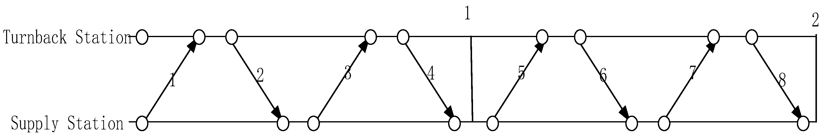
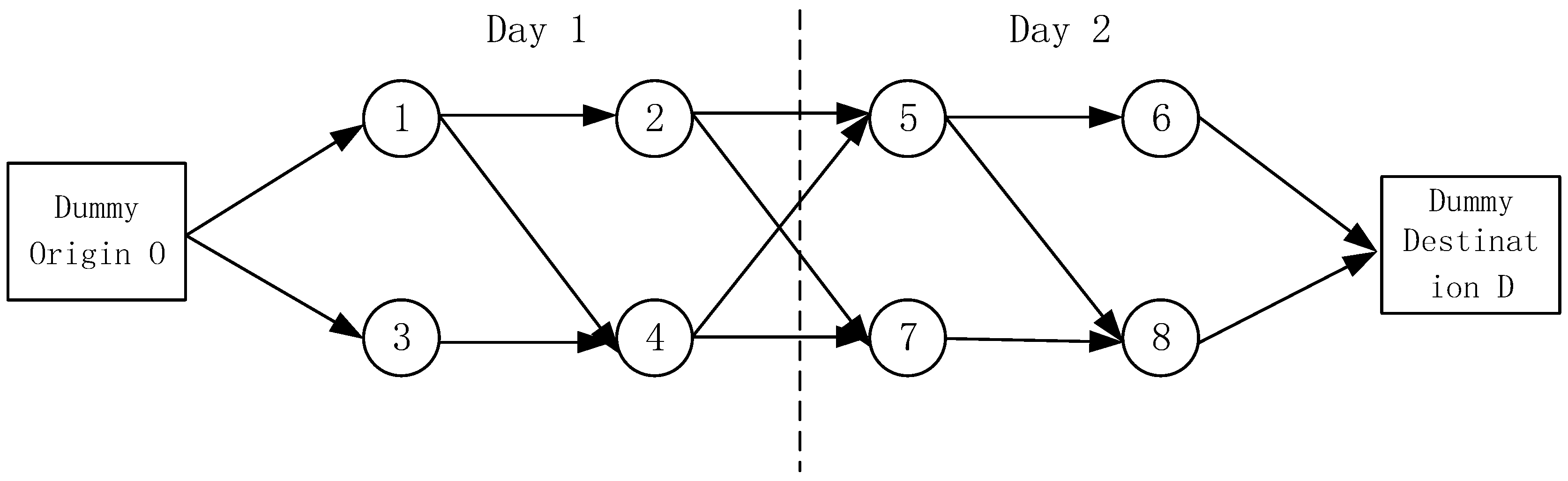
2. Problem Description
3. Optimization Model for the Routing Plan of Power-Concentrated EMUs
3.1. Symbol Specification
3.2. Model Assumptions
- Do not consider the limitations of the maintenance capacity of the depot.
- Do not consider EMU coupling and decoupling.
- Secondary repairs and above (D2-D6 repairs) are not considered.
3.3. Objective Function
3.4. Constraint
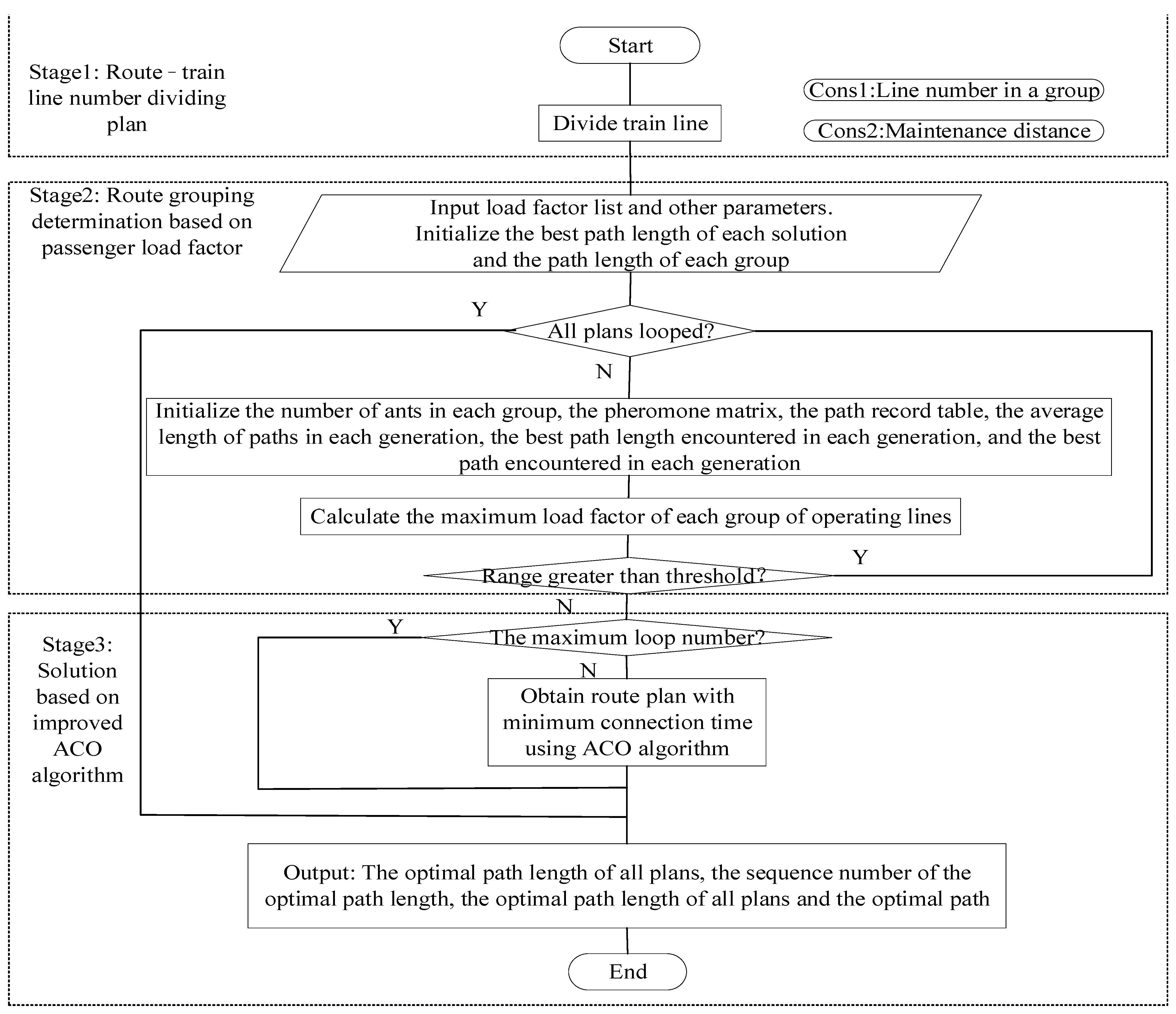
4. Route Optimization for Power-Concentrated EMUs Based on the Improved Ant Colony Algorithm
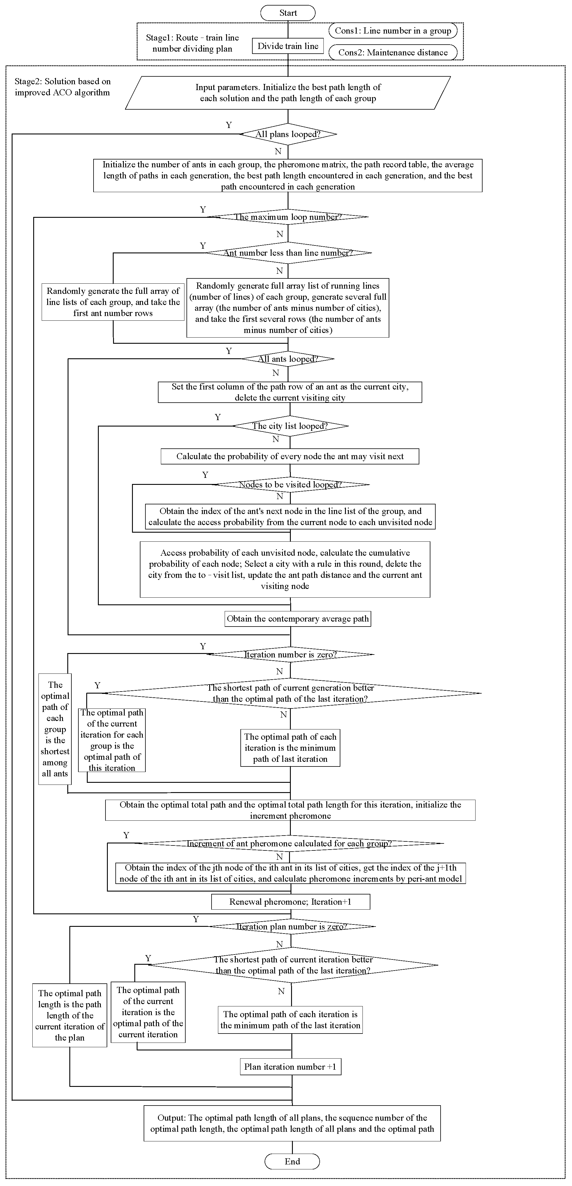
4.1. Algorithm Description
| Algorithm 1: Improved Ant Colony Algorithm for route optimization |
| Input: citydis, alpha, belta, ro, numcity, Q, itermax, iter1, heuris, listcity Output: lengthbest_s_total, pathbest_s_total Procedure for running line division select_city for s in select_city: for t in s: remove t from listcity obtain numcity Procedure for running line division Input numant iter=0 while iter<itermax: for i in range(numant): visiting=pathtable[i,0] remove visiting from unvisited for j in range(numcity): for k in range(listunvisited): choose city according to roulette rule update lengthbest_s_total and pathbest_s_total update pheromone according to Formula (13) iter+1 s_num+1 |
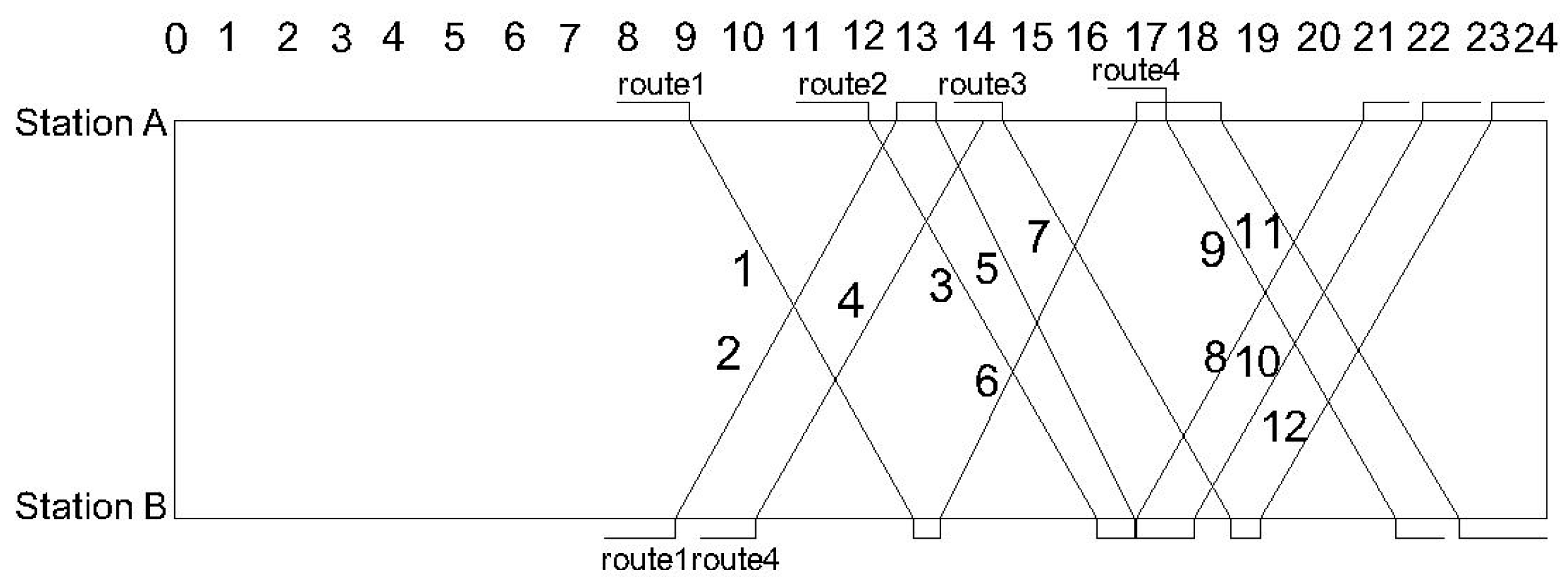
4.2. Case Study
4.2.1. Basic Experimental Data
4.2.2. Experimental Results
4.2.3. Extended Experiment—Route Optimization for EMUs Considering Passenger Flow Demand
| Algorithm 2: Improved Ant Colony Algorithm for route optimization considering the load factor rate |
| Input: citydis, alpha, belta, ro, numcity, Q, itermax, iter1, heuris, listcity, kezuolv Output: lengthbest_s_total, pathbest_s_total Procedure for running line division select_city for s in select_city: maxkezuolv=max(kezuolv1) minkezuolv=min(kezuolv1) jicha=maxkezuolv-minkezuolv if(jicha>threshold): continue for t in s: remove t from listcity obtain numcity Procedure for running line division Input numant iter=0 while iter<itermax: for i in range(numant): visiting=pathtable[i,0] remove visiting from unvisited for j in range(numcity): for k in range(listunvisited): choose city according to roulette rule update lengthbest_s_total and pathbest_s_total update pheromone according to Formula (13) iter+1 s_num+1 |
5. Route Evaluation for Power-Concentrated EMUs
5.1. Selection of Route Evaluation Indexes for Power-Concentrated EMUs
5.1.1. Operational Efficiency Index
- Number of routes ():
- Number of D1 repairs ():
- Minimum total connection time () (excluding the connection time when returning to the starting point, i.e., the D1 repair time):
- Total turnaround time for routing ():
- Average turnaround time for routing ():
- Number of days ():
- Number of train units ():
- Average route mileage ():
- Average route distance loss ():
- Vehicle kilometers per day ():
- Average daily occupancy time ():
- Utilization rate of EMUs ():
- 13.
- Average connection time between trains ():
- 14.
- Average number of tasks performed by EMUs ():
- 15.
- Minimum mileage of EMUs ():
- 16.
- Maximum mileage of EMUs ():
5.1.2. Balance Indicators
- 1.
- Route mileage balance ():
- 2.
- Variance of route utilization ():
5.1.3. Load Factor Consistency
- 1.
- Route average load factor range ():
- 2.
- Route mean standard deviation of the load factor ():
5.2. Plan Evaluation Based on the Entropy Weight–TOPSIS Method
- 1.
- Construction of a standard matrix.
- 2.
- The ratio of each index is found for each plan.
- 3.
- The information entropy of each index is found.
- 4.
- The weight of each indicator is determined.
- 5.
- The weighted standardized matrix is constructed.
- 6.
- The positive and negative ideal solutions are found.
- 7.
- The positive and negative ideal solution distances of objects are calculated.
- 8.
- The relative proximity is calculated and sorted.
6. Conclusions
Author Contributions
Funding
Data Availability Statement
Conflicts of Interest
References
- Haahr, J.T.; Wagenaar, J.C.; Veelenturf, L.P.; Kroon, L.G. A Comparison of Two Exact Methods for Passenger Railway Rolling Stock (re)scheduling. Transp. Res. Part E Logist. Transp. Rev. 2016, 9, 15–32. [Google Scholar] [CrossRef]
- Giacco, G.L.; D’Ariano, A.; Pacciarelli, D. Rolling Stock Rostering Optimization under Maintenance Constraints. Intell. Transp. Syst. 2014, 18, 95–105. [Google Scholar] [CrossRef]
- Abbink, E.; Van den Berg, B.; Kroon, L.; Salomon, M. Allocation of Railway Rolling Stock for Passenger Trains. Transp. Sci. 2004, 38, 33–41. [Google Scholar] [CrossRef]
- Alfieri, A.; Groot, R.; Kroon, L.; Schrijver, A. Efficient Circulation of Railway Rolling Stock. Transp. Sci. 2006, 40, 378–391. [Google Scholar] [CrossRef]
- Borndörfer, R.; Reuther, M.; Schlechte, T.; Waas, K.; Weider, S. Integrated Optimization of Rolling Stock Rotations for Intercity Railways. Transp. Sci. 2016, 50, 863–877. [Google Scholar] [CrossRef]
- Cacchiani, V.; Caprara, A.; Toth, P. An Effective Peak Period Heuristic for Railway Rolling Stock Planning. Transp. Sci. 2019, 53, 746–762. [Google Scholar] [CrossRef]
- Hong, S.P.; Kim, K.M.; Lee, K.; Park, B.H. A pragmatic algorithm for the train-set routing: The case of Korea high-speed railway. Omega 2009, 37, 637–645. [Google Scholar] [CrossRef]
- Song, H.; Li, L.; Li, Y.; Tan, L.; Dong, H. Functional Safety and Performance Analysis of Autonomous Route Management for Autonomous Train Control System. IEEE Trans. Intell. Transp. Syst. 2024, 25, 13291–13304. [Google Scholar] [CrossRef]
- Hoogervorst, R.; Dollevoet, T.; Maróti, G.; Huisman, D. A Variable Neighborhood Search Heuristic for Rolling Stock Rescheduling. EURO J. Transp. Logist. 2021, 10, 100032. [Google Scholar] [CrossRef]
- del Castillo, A.C.; Marcos, J.A.; Parlikad, A.K. Dynamic fleet maintenance management model applied to rolling stock. Reliab. Eng. Syst. Saf. 2023, 240, 109607. [Google Scholar] [CrossRef]
- Folco, P.; Malaguti, E.; Sahli, A.; Belmokhtar-Berraf, S.; Bouillaut, L. A flow formulation for the rolling stock maintenance scheduling problem. IFAC Pap. 2024, 58, 516–521. [Google Scholar] [CrossRef]
- Prause, F.; Borndörfer, R.; Grimm, B.; Tesch, A. Approximating rolling stock rotations with integrated predictive maintenance. J. Rail Transp. Plan. Manag. 2024, 30, 100434. [Google Scholar] [CrossRef]
- Pascariu, B.; Sama, M.; Pellegrini, P.; d’Ariano, A.; Rodriguez, J.; Pacciarelli, D. Formulation of train routing selection problem for different real-time traffic management objectives. J. Rail Transp. Plan. Manag. 2024, 31, 100460. [Google Scholar] [CrossRef]
- Kato, S.; Nakahigashi, T.; Kokubo, T.; Imaizumi, J. Rolling Stock Scheduling Algorithm for Temporary Timetable After Natural Disaster. Q. Rep. RTRI 2024, 65, 182–187. [Google Scholar] [CrossRef]
- Folco, P.; Sahli, A.; Belmokhtar-Berraf, S.; Bouillaut, L. A rolling horizon for rolling stock maintenance scheduling problem with cyclical activities. Comput. Ind. Eng. 2024, 196, 110460. [Google Scholar] [CrossRef]
- Amorosi, L.; Dell’Olmo, P.; Giacco, G.L. An integrated model for high-speed rolling-stock planning and maintenance scheduling. Eng. Optim. 2024, 56, 811–832. [Google Scholar] [CrossRef]
- Pan, H.; Yang, L.; Liang, Z.; Yang, H. New Exact Algorithm for the integrated train timetabling and rolling stock circulation planning problem with stochastic demand. Eur. J. Oper. Res. 2024, 316, 906–929. [Google Scholar] [CrossRef]
- Lin, B.; Shen, Y.; Zhong, W.; Wang, Z.; Guo, Q. Optimization of the Electric Multiple Units Circulation Plan with the Minimum Number of Train-Set. China Railw. Sci. 2023, 44, 210–221. [Google Scholar]
- Song, H.; Gao, S.; Li, Y.; Liu, L.; Dong, H. Train-centric communication based autonomous train control system. IEEE Trans. Intell. Veh. 2023, 8, 721–731. [Google Scholar] [CrossRef]


| Symbol | Meaning |
|---|---|
| Route division plan number, , represents a set of routing plans | |
| Sub-plan sequence number, | |
| Routing number, , represents a routing set | |
| Running line number, , represents a set of train lines, | |
| Edge set, where the available nodes are represented as , , represents a set of node pairs |
| Symbol | Meaning |
|---|---|
| Weight of the connection edge, that is, the connection time, min, , is a weight set | |
| Number of running lines in a route | |
| Number of routes in a sub-plan | |
| Number of routing division plans | |
| Mileage of running line | |
| Departure time of running line | |
| Arrival time of a running line | |
| Minimum turn-back time including the necessary time for the train turnaround time and the operation preparation time, which is 15 min here | |
| A sufficiently large number | |
| First-class repair (D1 repair) mileage cycle | |
| First-class repair (D1 repair) time cycle |
| Symbol | Meaning |
|---|---|
| If the running line is connected to the running line , , otherwise, | |
| Total train units in sub-plan | |
| Total turnaround time for routing | |
| The minimum total connection time of all routes in the sub-plan | |
| Auxiliary decision variable | |
| The cumulative mileage of the route | |
| The cumulative running time of the route |
| Train Number | Arrive/Depart | Station | Train Number | Arrive/Depart | Station | ||
|---|---|---|---|---|---|---|---|
| Station A | Station B | Station A | Station B | ||||
| 1 | Arrive | — | 12:55 | 2 | Arrive | — | 12:38 |
| Depart | 9:00 | — | Depart | 8:45 | — | ||
| 3 | Arrive | — | 16:08 | 4 | Arrive | — | 14:10 |
| Depart | 12:08 | — | Depart | 10:10 | — | ||
| 5 | Arrive | — | 16:48 | 6 | Arrive | — | 16:50 |
| Depart | 13:20 | — | Depart | 13:24 | — | ||
| 7 | Arrive | — | 18:28 | 8 | Arrive | — | 20:48 |
| Depart | 14:29 | — | Depart | 16:50 | — | ||
| 9 | Arrive | — | 21:22 | 10 | Arrive | — | 21:50 |
| Depart | 17:20 | — | Depart | 17:50 | — | ||
| 11 | Arrive | — | 22:29 | 12 | Arrive | — | 23:03 |
| Depart | 18:18 | — | Depart | 19:00 | — | ||
| Initial Pheromone Concentrations for All Paths | Pheromone Importance Factor | Heuristic Function Importance Factor | Volatilization Coefficient | Total Pheromone | Cycle Maximum |
|---|---|---|---|---|---|
| 1 | 1 | 5 | 0.1 | 1 | 200 |
| Plan Number | Route Number | Line Division | Minimum Total Connection Time/min | Optimum Routing |
|---|---|---|---|---|
| 1 | 2 | (8, 4) | 2372 | 3−8−1−6−9−2−5−10, 11−4−7−12 |
| 2 | 3 | (8, 2, 2) | 1698 | 7−12−1−6−11−2−5−10, 3−8, 4−9 |
| 3 | 2 | (6, 6) | 2327 | 4−7−12−1−6−9, 11−2−5−10−3−8 |
| 4 | 3 | (6, 4, 2) | 1469 | 4−7−12−1−6−9, 11−2−5−10, 3−8 |
| 5 | 4 | (6, 2, 2, 2) | 1101 | 1−6−11−2−5−10, 3−8, 4−9, 7−12 |
| 6 | 3 | (4, 4, 4) | 2342 | 3−8−1−6, 9−2−5−10, 11−4−7−12 |
| 7 | 4 | (4, 4, 2, 2) | 1437 | 12−1−6−9, 11−2−5−10, 3−8, 4−7 |
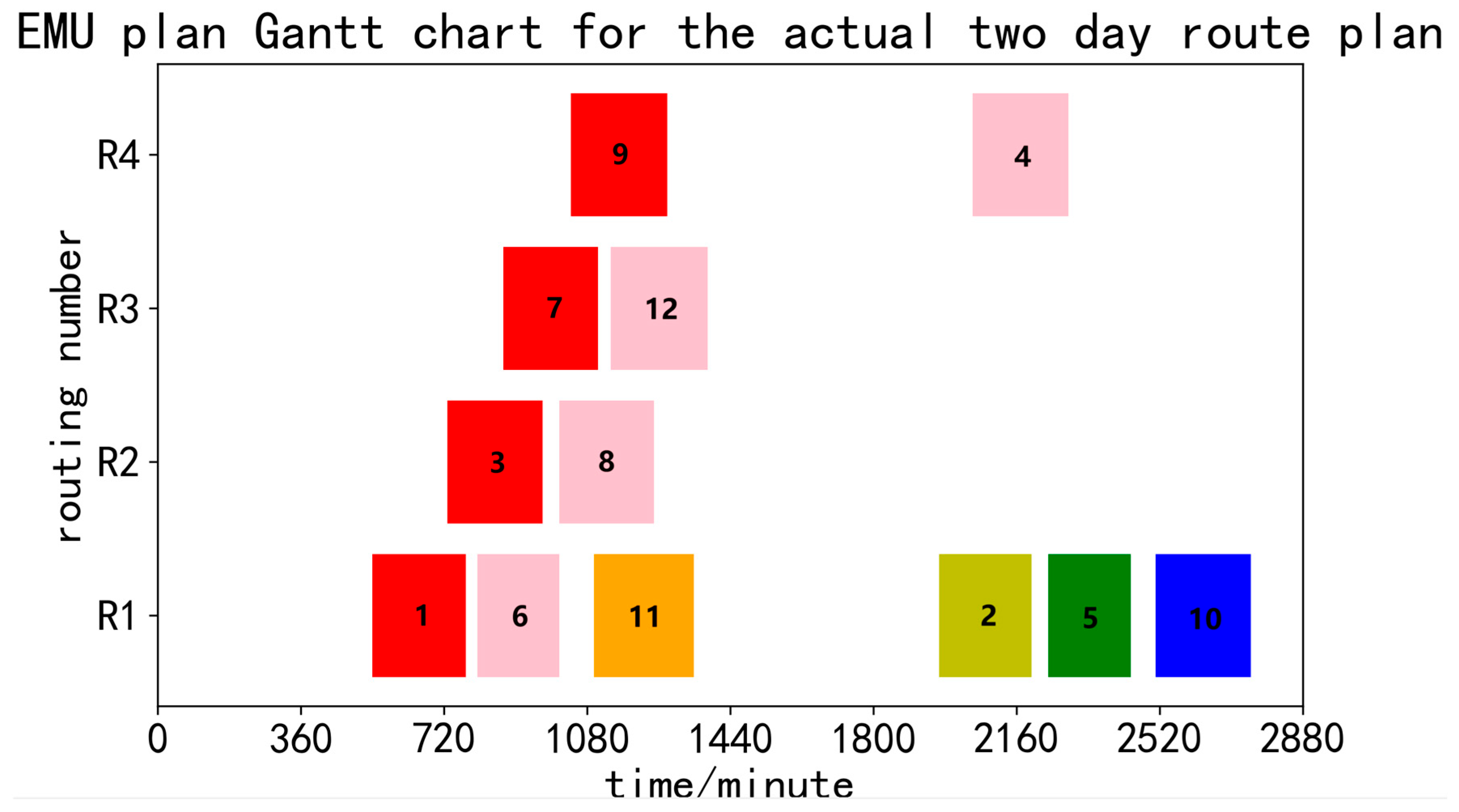
| Actual plan | 4 | (6, 2, 2, 2) | 1679 | 1−6−11−2−5−10, 3−8, 7−12, 9−4 |
| Parameter Analysis Plan | Parameter | Calculation Index | ||||
|---|---|---|---|---|---|---|
| Ant Number | Pheromone Importance Factor | Heuristic Function Importance Factor | Iteration Number | Minimum Connection time/min | Calculation Time/s | |
| P1 | 18 | 1 | 5 | 200 | 2372 | 242.6850514412 |
| P2 | 6 | 1 | 5 | 200 | 2372 | 51.7229347229 |
| P3 | 12 | 1 | 5 | 200 | 2372 | 389.9291911125 |
| P4 | 24 | 1 | 5 | 200 | 2372 | 634.6604983807 |
| P5 | 18 | 0.5 | 5 | 200 | 2372 | 654.1037375927 |
| P6 | 18 | 2 | 5 | 200 | 2372 | 914.2404844761 |
| P7 | 18 | 3 | 5 | 200 | 2372 | 432.2556602955 |
| P8 | 18 | 4 | 5 | 200 | No solution | -- |
| P9 | 18 | 5 | 5 | 200 | No solution | -- |
| P10 | 18 | 1 | 2 | 200 | 2372 | 885.7629337311 |
| P11 | 18 | 1 | 3 | 200 | 2372 | 491.3823523521 |
| P12 | 18 | 1 | 4 | 200 | 2372 | 601.4855833054 |
| P13 | 18 | 1 | 6 | 200 | 2372 | 247.1675834656 |
| P14 | 18 | 1 | 5 | 10 | 2372 | 8.1696150303 |
| P15 | 18 | 1 | 5 | 50 | 2372 | 36.9381115437 |
| P16 | 18 | 1 | 5 | 100 | 2372 | 73.2007288933 |
| P17 | 18 | 1 | 5 | 150 | 2372 | 109.4171283245 |
| Symbol | Meaning |
|---|---|
| Load rate of |
| Train Number | Load Factor/% | Train Number | Load Factor/% | Train Number | Load Factor/% | Train Number | Load Factor/% | Train Number | Load Factor/% | Train Number | Load Factor/% |
|---|---|---|---|---|---|---|---|---|---|---|---|
| 1 | 50 | 2 | 60 | 3 | 90 | 4 | 80 | 5 | 50 | 6 | 50 |
| 7 | 80 | 8 | 80 | 9 | 50 | 10 | 60 | 11 | 80 | 12 | 80 |
| Plan Number | Route Number | Line Division | Route Load Factor Range Threshold | Number of Plans Meeting the Load Factor Connection Condition | Minimum Total Connection Time/min | Optimal Routing | Route Average Range of Passenger Load Factor |
|---|---|---|---|---|---|---|---|
| 1−1 | 2 | (8, 4) | 10% | 0 | — | — | — |
| 1−2 | 20% | 0 | — | — | — | ||
| 1−3 | 30% | 36 | 2556 | 4−11−2−5−10−1−6−9, 7−12−3−8 | 20% | ||
| 1−4 | 40% | 495 | 2372 | 3−8−1−6−9−2−5−10, 11−4−7−12 | 20% | ||
| 1−5 | 100% | 495 | 2372 | 3−8−1−6−9−2−5−10, 11−4−7−12 | 20% | ||
| 2−1 | 3 | (8, 2, 2) | 10% | — | — | — | — |
| 2−2 | 20% | — | — | — | — | ||
| 2−3 | 30% | 636 | 1698 | 7−12−1−6−11−2−5−10, 3−8, 4−9 | 23% | ||
| 2−4 | 40% | 2970 | 1698 | 7−12−1−6−11−2−5−10, 3−8, 4−9 | 23% | ||
| 2−5 | 100% | 2970 | 1698 | 7−12−1−6−11−2−5−10, 3−8, 4−9 | 23% | ||
| 3−1 | 2 | (6, 6) | 10% | 2 | 2412 | 2−5−10−1−6−9, 11−4−7−12−3−8 | 10% |
| 3−2 | 20% | 2 | 2412 | 2−5−10−1−6−9, 11−4−7−12−3−8 | 10% | ||
| 3−3 | 30% | 42 | 2412 | 2−5−10−1−6−9, 11−4−7−12−3−8 | 10% | ||
| 3−4 | 40% | 924 | 2327 | 4−7−12−1−6−9, 11−2−5−10−3−8 | 35% | ||
| 3−5 | 100% | 924 | 2327 | 4−7−12−1−6−9, 11−2−5−10−3−8 | 35% | ||
| 4−1 | 3 | (6, 4, 2) | 10% | 30 | 1627 | 2−5−10−1−6−9, 11−4−7−12, 3−8 | 7% |
| 4−2 | 20% | 35 | 1627 | 2−5−10−1−6−9, 11−4−7−12, 3−8 | 7% | ||
| 4−3 | 30% | 2765 | 1469 | 4−7−12−1−6−9, 11−2−5−10, 3−8 | 23% | ||
| 4−4 | 40% | 13,860 | 1469 | 4−7−12−1−6−9, 11−2−5−10, 3−8 | 23% | ||
| 4−5 | 100% | 13,860 | 1469 | 4−7−12−1−6−9, 11−2−5−10, 3−8 | 23% | ||
| 5−1 | 4 | (6, 2, 2, 2) | 10% | 180 | 1155 | 2−5−10−1−6−9, 3−8, 4−11, 7−12 | 5% |
| 5−2 | 20% | 270 | 1155 | 2−5−10−1−6−9, 3−8, 4−11, 7−12 | 5% | ||
| 5−3 | 30% | 28,350 | 1101 | 1−6−11−2−5−10, 3−8, 4−9, 7−12 | 18% | ||
| 5−4 | 40% | 83,160 | 1101 | 1−6−11−2−5−10, 3−8, 4−9, 7−12 | 18% | ||
| 5−5 | 100% | 83,160 | 1101 | 1−6−11−2−5−10, 3−8, 4−9, 7−12 | 18% | ||
| 6−1 | 3 | (4, 4, 4) | 10% | — | — | — | — |
| 6−2 | 20% | 60 | — | — | — | ||
| 6−3 | 30% | 7350 | 2347 | 8−1−6−9, 11−2−5−10, 4−7−12−3 | 23% | ||
| 6−4 | 40% | 34,650 | 2342 | 3−8−1−6, 9−2−5−10, 11−4−7−12 | 17% | ||
| 6−5 | 100% | 34,650 | 2342 | 3−8−1−6, 9−2−5−10, 11−4−7−12 | 17% | ||
| 7−1 | 4 | (4, 4, 2, 2) | 10% | 900 | 1565 | 10−1−6−9, 11−4−7−12, 2−5, 3−8 | 8% |
| 7−2 | 20% | 1380 | 1565 | 10−1−6−9, 11−4−7−12, 2−5, 3−8 | 8% | ||
| 7−3 | 30% | 73,500 | 1437 | 12−1−6−9, 11−2−5−10, 3−8, 4−7 | 18% | ||
| 7−4 | 40% | 207,900 | 1437 | 12−1−6−9, 11−2−5−10, 3−8, 4−7 | 18% | ||
| 7−5 | 100% | 207,900 | 1437 | 12−1−6−9, 11−2−5−10, 3−8, 4−7 | 18% | ||
| Actual plan | 4 | (6, 2, 2, 2) | — | — | 1679 | 1−6−11−2−5−10, 3−8, 7−12, 9−4 | 18% |
| Primary Index | Secondary Index | Index Type |
|---|---|---|
| Operation Efficiency | Negative | |
| Number of D1 repairs | Negative | |
| Minimum total connection time | Negative | |
| Total turnaround time for routing | Negative | |
| Average turnaround time for routing | Negative | |
| Number of days | Negative | |
| Number of train units | Negative | |
| Average route mileage | Positive | |
| Average route distance loss | Negative | |
| Vehicle kilometers per day | Positive | |
| Average daily occupancy time | Positive | |
| Utilization rate of EMUs | Positive | |
| Average connection time between trains | Negative | |
| Average number of tasks performed by EMUs | Positive | |
| Minimum mileage of EMUs | Positive | |
| Maximum mileage of EMUs | Positive | |
| Operating Balance | Route mileage balance | Negative |
| Variance of route utilization | Negative | |
| Load Factor Consistency | Route average load factor range | Negative |
| Route mean standard deviation of the load factor | Negative |
| Plan Num | 1−3 | 1−4 | 2−3 | 3−1 | 3−4 | 4−1 | 4−3 |
|---|---|---|---|---|---|---|---|
| 2 | 2 | 3 | 2 | 2 | 3 | 3 | |
| 2 | 2 | 3 | 2 | 2 | 3 | 3 | |
/min | 2556 | 2372 | 1698 | 2412 | 2327 | 1627 | 1469 |
/min | 5371 | 5187 | 4513 | 5227 | 5142 | 4442 | 4284 |
/min | 2685.5 | 2593.5 | 1504.333 | 2613.5 | 2571 | 1480.667 | 1428 |
| 5 | 5 | 5 | 5 | 5 | 5 | 5 | |
| 5 | 5 | 5 | 5 | 5 | 5 | 5 | |
/km | 2826 | 2826 | 1884 | 2826 | 2826 | 1884 | 1884 |
/km | 1174 | 1174 | 2116 | 1174 | 1174 | 2116 | 2116 |
/km | 1130.4 | 1130.4 | 1130.4 | 1130.4 | 1130.4 | 1130.4 | 1130.4 |
/min | 563 | 563 | 563 | 563 | 563 | 563 | 563 |
| 0.390972222 | 0.390972 | 0.390972 | 0.390972 | 0.390972 | 0.390972 | 0.390972 | |
/min | 255.6 | 237.2 | 188.6667 | 241.2 | 232.7 | 180.7778 | 163.2222 |
| 6 | 6 | 4 | 6 | 6 | 4 | 4 | |
/km | 1884 | 1884 | 942 | 2826 | 2826 | 942 | 942 |
/km | 3768 | 3768 | 3768 | 2826 | 2826 | 2826 | 2826 |
| 1884 | 1884 | 2826 | 0 | 0 | 1884 | 1884 | |
| 0.002307112 | 0.00196 | 0.002052 | 0.004742 | 0.006517 | 0.004282 | 0.005705 | |
| 0.2 | 0.2 | 0.23 | 0.1 | 0.35 | 0.07 | 0.23 | |
| 0.03 | 0.03 | 0.06 | 0.02 | 0.06 | 0.02 | 0.05 | |
| Plan Num | 5−1 | 5−3 | 6−3 | 6−4 | 7−1 | 7−3 | 8 |
| 4 | 4 | 3 | 3 | 4 | 4 | 4 | |
| 4 | 4 | 3 | 3 | 4 | 4 | 4 | |
/min | 1155 | 1101 | 2347 | 2342 | 1437 | 1437 | 1679 |
/min | 3970 | 3916 | 5162 | 5157 | 4252 | 4252 | 4494 |
/min | 992.5 | 979 | 1720.667 | 1719 | 1063 | 1063 | 1123.5 |
| 5 | 5 | 6 | 6 | 6 | 6 | 5 | |
| 5 | 5 | 6 | 6 | 6 | 6 | 5 | |
/km | 1413 | 1413 | 1884 | 1884 | 1413 | 1413 | 1413 |
/km | 2587 | 2587 | 2116 | 2116 | 2587 | 2587 | 2587 |
/km | 1130.4 | 1130.4 | 942 | 942 | 942 | 942 | 1130.4 |
/min | 563 | 563 | 469.1667 | 469.1667 | 469.1667 | 469.1667 | 563 |
| 0.390972 | 0.390972 | 0.32581 | 0.32581 | 0.32581 | 0.32581 | 0.390972222 | |
/min | 144.375 | 137.625 | 260.7778 | 260.2222 | 179.625 | 179.625 | 209.875 |
| 3 | 3 | 4 | 4 | 3 | 3 | 3 | |
/km | 942 | 942 | 1884 | 1884 | 942 | 942 | 942 |
/km | 2826 | 2826 | 1884 | 1884 | 1884 | 1884 | 2826 |
| 1884 | 1884 | 0 | 0 | 942 | 942 | 1884 | |
| 0.003568 | 0.003832 | 3.62 × 10⁵ | 7.28 × 10⁵ | 2.42 × 10⁵ | 2.42 × 10⁵ | 0.003832247 | |
| 0.05 | 0.18 | 0.23 | 0.17 | 0.08 | 0.18 | 0.18 | |
| 0.02 | 0.05 | 0.05 | 0.04 | 0.02 | 0.04 | 0.05 |
| Index Range | Total | Operation Efficiency of EMU | EMU Operation Balance | Load Factor Consistency |
|---|---|---|---|---|
| Maximum Value | 0.7445 | 0.8216 | 0.5505 | 0.5589 |
| Plan Number | 3−1 | 1−3 | 6−3 and 6−4 | 3−1 |
| The Route Corresponding to the Plan | 1−4−9−0−5−8, 10−3−6−11−2−7 | 4−11−2−5−10−1−6−9, 7−12−3−8 | 8−1−6−9, 11−2−5−10, 4−7−12−3 and 3−8−1−6, 9−2−5−10, 11−4−7−12 | 2−5−10−1−6−9, 11−4−7−12−3−8 |
| Minimum Value | 0.2408 | 0.1183 | 0.3276 | 0.0000 |
| Plan Number | 7−3 | 7−1 and 7−3 | 4−3 | 3−4 |
| The Route Corresponding to the Plan | 11−0−5−8, 10−1−4−9, 2−7, 3−6 | 10−1−6−9, 11−4−7−12, 2−5, 3−8 and 12−1−6−9, 11−2−5−10, 3−8, 4−7 | 4−7−12−1−6−9, 11−2−5−10, 3−8 | 4−7−12−1−6−9, 11−2−5−10−3−8 |
| Index | U1 | U2 | U3 | U4 | U5 | U6 | U7 | U8 | U9 | U10 |
| 1-3 | 50.0% | 50.0% | −52.2% | −19.5% | −139.0% | 0.0% | 0.0% | 100.0% | 54.6% | 0.0% |
| 1-4 | 50.0% | 50.0% | −41.3% | −15.4% | −130.8% | 0.0% | 0.0% | 100.0% | 54.6% | 0.0% |
| 2-3 | 25.0% | 25.0% | −1.1% | −0.4% | −33.9% | 0.0% | 0.0% | 33.3% | 18.2% | 0.0% |
| 3-1 | 50.0% | 50.0% | −43.7% | −16.3% | −132.6% | 0.0% | 0.0% | 100.0% | 54.6% | 0.0% |
| 3-4 | 50.0% | 50.0% | −38.6% | −14.4% | −128.8% | 0.0% | 0.0% | 100.0% | 54.6% | 0.0% |
| 4-1 | 25.0% | 25.0% | 3.1% | 1.2% | −31.8% | 0.0% | 0.0% | 33.3% | 18.2% | 0.0% |
| 4-3 | 25.0% | 25.0% | 12.5% | 4.7% | −27.1% | 0.0% | 0.0% | 33.3% | 18.2% | 0.0% |
| 5-1 | 0.0% | 0.0% | 31.2% | 11.7% | 11.7% | 0.0% | 0.0% | 0.0% | 0.0% | 0.0% |
| 5-3 | 0.0% | 0.0% | 34.4% | 12.9% | 12.9% | 0.0% | 0.0% | 0.0% | 0.0% | 0.0% |
| 6-3 | 25.0% | 25.0% | −39.8% | −14.9% | −53.2% | −20.0% | −20.0% | 33.3% | 18.2% | −16.7% |
| 6-4 | 25.0% | 25.0% | −39.5% | −14.8% | −53.0% | −20.0% | −20.0% | 33.3% | 18.2% | −16.7% |
| 7-1 | 0.0% | 0.0% | 14.4% | 5.4% | 5.4% | −20.0% | −20.0% | 0.0% | 0.0% | −16.7% |
| 7-3 | 0.0% | 0.0% | 14.4% | 5.4% | 5.4% | −20.0% | −20.0% | 0.0% | 0.0% | −16.7% |
| Actual Plan | 1 | 1 | 1 | 1 | 1 | 1 | 1 | 1 | 1 | 1 |
| Index | U11 | U12 | U13 | U14 | U15 | U16 | U17 | U18 | U19 | U20 |
| 1-3 | 0.0% | 0.0% | −21.8% | 100.0% | 100.0% | 33.3% | 0.0% | 39.8% | −11.1% | 40.0% |
| 1-4 | 0.0% | 0.0% | −13.0% | 100.0% | 100.0% | 33.3% | 0.0% | 48.9% | −11.1% | 40.0% |
| 2-3 | 0.0% | 0.0% | 10.1% | 33.3% | 0.0% | 33.3% | −50.0% | 46.5% | −27.8% | −20.0% |
| 3-1 | 0.0% | 0.0% | −14.9% | 100.0% | 200.0% | 0.0% | 100.0% | −23.8% | 44.4% | 60.0% |
| 3-4 | 0.0% | 0.0% | −10.9% | 100.0% | 200.0% | 0.0% | 100.0% | −70.1% | −94.4% | −20.0% |
| 4-1 | 0.0% | 0.0% | 13.9% | 33.3% | 0.0% | 0.0% | 0.0% | −11.7% | 61.1% | 60.0% |
| 4-3 | 0.0% | 0.0% | 22.2% | 33.3% | 0.0% | 0.0% | 0.0% | −48.9% | −27.8% | 0.0% |
| 5-1 | 0.0% | 0.0% | 31.2% | 0.0% | 0.0% | 0.0% | 0.0% | 6.9% | 72.2% | 60.0% |
| 5-3 | 0.0% | 0.0% | 34.4% | 0.0% | 0.0% | 0.0% | 0.0% | 0.0% | 0.0% | 0.0% |
| 6-3 | −16.7% | −16.7% | −24.3% | 33.3% | 100.0% | −33.3% | 100.0% | 99.1% | −27.8% | 0.0% |
| 6-4 | −16.7% | −16.7% | −24.0% | 33.3% | 100.0% | −33.3% | 100.0% | 98.1% | 5.6% | 20.0% |
| 7-1 | −16.7% | −16.7% | 14.4% | 0.0% | 0.0% | −33.3% | 50.0% | 99.4% | 55.6% | 60.0% |
| 7-3 | −16.7% | −16.7% | 14.4% | 0.0% | 0.0% | −33.3% | 50.0% | 99.4% | 0.0% | 20.0% |
| Actual Plan | 1 | 1 | 1 | 1 | 1 | 1 | 1 | 1 | 1 | 1 |
Disclaimer/Publisher’s Note: The statements, opinions and data contained in all publications are solely those of the individual author(s) and contributor(s) and not of MDPI and/or the editor(s). MDPI and/or the editor(s) disclaim responsibility for any injury to people or property resulting from any ideas, methods, instructions or products referred to in the content. |
© 2025 by the authors. Licensee MDPI, Basel, Switzerland. This article is an open access article distributed under the terms and conditions of the Creative Commons Attribution (CC BY) license (https://creativecommons.org/licenses/by/4.0/).
Share and Cite
Wang, Y.; Xu, L.; Yang, X.; Bao, J.; Lin, F.; Guo, Y.; Yue, Y. Scheduling and Evaluation of a Power-Concentrated EMU on a Conventional Intercity Railway Based on the Minimum Connection Time. Mathematics 2025, 13, 508. https://doi.org/10.3390/math13030508
Wang Y, Xu L, Yang X, Bao J, Lin F, Guo Y, Yue Y. Scheduling and Evaluation of a Power-Concentrated EMU on a Conventional Intercity Railway Based on the Minimum Connection Time. Mathematics. 2025; 13(3):508. https://doi.org/10.3390/math13030508
Chicago/Turabian StyleWang, Yinan, Limin Xu, Xiao Yang, Jingjing Bao, Feng Lin, Yiwei Guo, and Yixiang Yue. 2025. "Scheduling and Evaluation of a Power-Concentrated EMU on a Conventional Intercity Railway Based on the Minimum Connection Time" Mathematics 13, no. 3: 508. https://doi.org/10.3390/math13030508
APA StyleWang, Y., Xu, L., Yang, X., Bao, J., Lin, F., Guo, Y., & Yue, Y. (2025). Scheduling and Evaluation of a Power-Concentrated EMU on a Conventional Intercity Railway Based on the Minimum Connection Time. Mathematics, 13(3), 508. https://doi.org/10.3390/math13030508