MHD Taylor–Couette Flow of Oldroyd-B Fluids Through a Porous Medium in an Annulus Induced by Time-Dependent Couples

Abstract

The Taylor–Couette flow of electrically conducting incompressible Oldroyd-B fluids induced by time-dependent couples in an annulus is analytically investigated when magnetic and porous effects are taken into account. Closed-form expressions are established for the dimensionless shear stress, fluid velocity and Darcy’s resistance by means of the integral transforms. Similar solutions for the MHD Taylor–Couette flow of the same fluids through a porous medium induced by a time-dependent couple in an infinite circular cylinder are obtained as limiting cases of previous results. In both cases, the obtained results can generate exact solutions for any motion of this kind of the respective fluids. Consequently, the two MHD motions of the respective fluids through a porous medium are completely solved. For illustration, two case studies are considered and the fluid behavior is graphically investigated. The convergence of the starting solutions to their permanent components is proved and the required time to touch the permanent state is determined.

1. Introduction

The rheological behavior of concentrated and molten polymer solutions is adequately described by the Oldroyd-B constitutive model. Respective fluids can be used, for instance, in water filtration systems, oil reservoirs and biomedical fields. This model, whose constitutive equations contain three material constants, is amenable to analysis and has been extensively studied along the time. The earliest precise solutions for unsteady flows of incompressible Oldroyd-B fluids with practical significance in cylindrical domains were provided by Waters and King [1]. Interesting results on this have been obtained by Rajagopal and Bhatnagar [2], Wood [3], Fetecau [4], McGinty et al. [5], Corina Fetecau et al. [6], Jamil and Khan [7], Imran et al. [8], and Ullah et al. [9]. Obtained solutions, which can bring to light the fluid behavior in different motion situations, can also be used to test numerical schemes that are developed for more complex flow problems.

Magnetohydrodynamic (MHD) motions of electrically conducting fluids have different applications in the manufacturing of polymers, MHD generators, biological fluids, plasma studies, nuclear reactors, and hydrology. The interaction between an electrically conducting fluid in motion and a magnetic field leads to significant effects in physics, chemical and engineering applications. Khan et al. [10], Zahid et al. [11] and Ghosh et al. [12] have studied motions of electrically conducting incompressible Oldroyd-B fluids (ECIOBFs) in rectangular domains. The motions of fluids through porous media have applications in different domains like the petroleum industry, astrophysics, composite manufacturing processes, geophysics, and many others. Tan and Masuoka [13], Khan et al. [14], Hayat et al. [15], Sultan et al. [16], and Khan and Ijaz [17] have made important contributions regarding MHD motions of ECIOBFs in rectangular domains. Unfortunately, the motions of the same fluids in cylindrical domains have not been sufficiently studied. The exact solutions for such motions were obtained by Hayat et al. [18], Hamza [19], Riaz et al. [20], Fetecau and Vieru [21], and Fetecau et al. [22].

The main purpose of the present study is to develop exact general solutions for MHD Taylor–Couette flow of ECIOBFs through a porous medium between two infinite circular coaxial cylinders induced by time-dependent couples. Exact solutions for the same flow of incompressible second grade fluids in an annulus induced by a constant couple have been established by Bandelli and Rajagopal [23]. Here, general expressions are established for the shear stress and the corresponding velocity field. The MHD Taylor–Couette flow of ECIOBFs through a porous medium in an infinite circular cylinder that applies a time-dependent couple to the fluid is also investigated and the corresponding solutions are obtained as limiting cases of previous results. Finally, two particular motions are considered, and the corresponding solutions are used to determine the time required to touch the permanent state and to underline some characteristics of fluid motion.

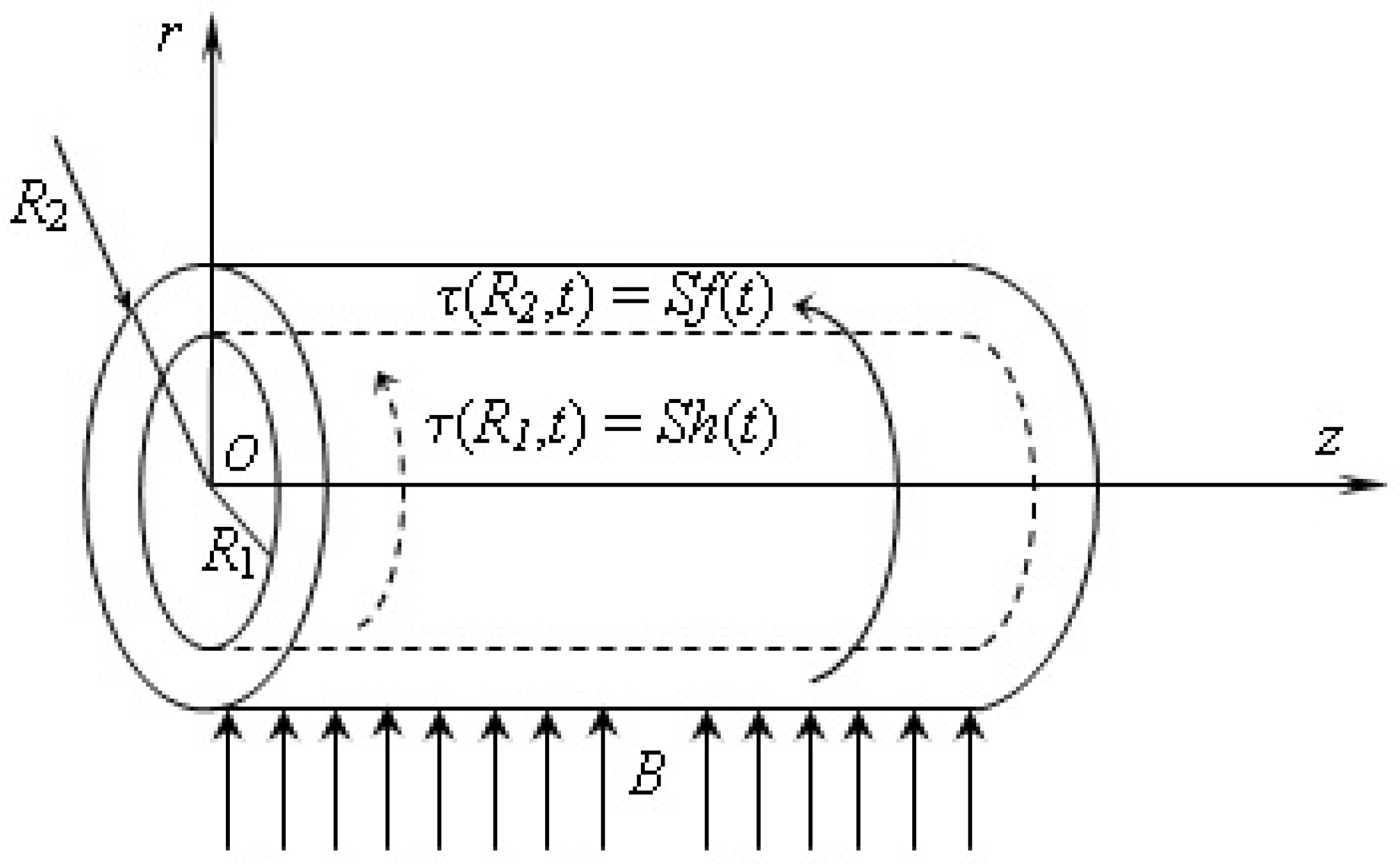
2. Problem Presentation

Let us assume that an ECIOBF, whose constitutive equations are given by following relations [24],

$$\mathit{T}=-p\mathit{I}+\mathit{S},$$

(1)

$$S+\lambda {\displaystyle \frac{DS}{Dt}}=2\mu \left(\mathit{D}+{\lambda }_r{\displaystyle \frac{D\mathit{D}}{Dt}}\right),$$

(2)

is at rest in a porous medium between two infinite coaxial circular cylinders of radii $R_1$ and $R_2$ $(>R_1).$ Here, T is the stress tensor, S is the extra-stress tensor, $\mathit{D}=[\mathrm{grad}\mathit{V}+{(\mathrm{grad}\mathit{V})}^T]/2$ is the rate of deformation tensor and $\mathit{V}$ is the velocity vector, I is the unit tensor, p is the hydrostatic pressure, $\mu$ is the fluid viscosity, $\lambda$ and ${\lambda }_r$ are relaxation and retardation times, respectively, and D/Dt is the time upper-convected derivative. When the constant ${\lambda }_r=0$ or $\lambda ={\lambda }_r=0$, the governing Equation (1) defines electrically conducting incompressible Maxwell or Newtonian fluids, respectively.

At the moment $t=0^{+}$, the two cylinders begin to rotate around their common symmetry axis due to the time-dependent torques $2\pi R_{1}Sh(t)$ and $2\pi R_{2}Sf(t)$, which are applied per unit length of the two cylinders. Here, S is a constant shear stress, while the piecewise continuous functions $h(\cdot )$ and $f(\cdot )$ have the zero value for $t=0$. A circular magnetic field of constant strength B acts perpendicular to the symmetry axis of the two cylinders, like in Figure 1.

Due to the shear, the fluid begins to move and the balance of linear momentum is expressed by the next relation:

$$\rho {\displaystyle \frac{d\mathit{V}}{dt}}=-gradp+\mathrm{div}\mathit{S}+\mathit{R}+{\mathit{F}}_e,$$

(3)

where $\rho$ is the fluid density, R is the Darcy’s resistance, and ${\mathit{F}}_e$ is the electromagnetic force [21,25].

In the following, we assume that the induced magnetic field can be neglected, the magnetic permeability of the fluid is constant, the electric field imposed is zero, and there is no surplus electric charge distribution in the fluid. In these conditions, the electromagnetic force ${\mathit{F}}_e$ is proportional to the velocity vector, i.e., [21,25]:

$${\mathit{F}}_e=-\sigma B^2\mathit{V},$$

(4)

where $\sigma$ is the electrical conductivity of the fluid. In addition, the Darcy’s resistance R for isothermal motions of ECIOBFs satisfies the following differential Equation [19]:

$$\left(1+\lambda {\displaystyle \frac{\partial }{\partial t}}\right)\mathit{R}=-\mu {\displaystyle \frac{\varphi }{k}}\left(1+{\lambda }_r{\displaystyle \frac{\partial }{\partial t}}\right)\mathit{V},$$

(5)

in which $\varphi \hspace{0.17em}(0<\varphi <1)$ and $k\hspace{0.17em}(>0)$ are the porosity and the permeability of porous medium.

Since the two cylinders are infinite in length and have the same symmetry axis, all physical entities characterizing this motion are functions of r and t only in a convenient system of cylindrical co-ordinates r, $\theta$ and z. In the following, as well as in the work of Bandelli and Rajagopal [23], we look for a velocity vector field of the following form:

$$\mathit{V}=\mathit{V}(r,t)=\left(0,w(r,t),0\right).$$

(6)

Substituting $\mathit{V}(r,t)$ from Equation (6) in (2) and taking into account that the fluid was at rest up to the initial moment $t=0$, one finds:

$$\left(1+\lambda {\displaystyle \frac{\partial }{\partial t}}\right)\tau (r,t)=\mu \left(1+{\lambda }_r{\displaystyle \frac{\partial }{\partial t}}\right)\left({\displaystyle \frac{\partial }{\partial r}}-{\displaystyle \frac{1}{r}}\right)w(r,t);\hspace{0.17em}\hspace{0.17em}\hspace{0.17em}\hspace{0.17em}{R}_1<r<R_2,\hspace{0.17em}\hspace{0.17em}\hspace{0.17em}\hspace{0.17em}t>0,$$

(7)

where $\tau (r,t)=S_{r\theta }(r,t)$ is the non-null component of the extra stress tensor S.

The continuity equation is satisfied while the motion in Equations (3) and (5) for Darcy’s resistance is reduced to the following scalar forms:

$$\rho {\displaystyle \frac{\partial w(r,t)}{\partial t}}=\left({\displaystyle \frac{\partial }{\partial r}}+{\displaystyle \frac{2}{r}}\right)\tau (r,t)-\sigma B^{2}w(r,t)+R(r,t);\hspace{0.17em}\hspace{0.17em}\hspace{0.17em}\hspace{0.17em}{R}_1<r<R_2,\hspace{0.17em}\hspace{0.17em}\hspace{0.17em}\hspace{0.17em}t>0,$$

(8)

$$\left(1+\lambda {\displaystyle \frac{\partial }{\partial t}}\right)R(r,t)=-\mu {\displaystyle \frac{\varphi }{k}}\left(1+{\lambda }_r{\displaystyle \frac{\partial }{\partial t}}\right)w(r,t);\hspace{0.17em}\hspace{0.17em}\hspace{0.17em}\hspace{0.17em}{R}_1<r<R_2,\hspace{0.17em}\hspace{0.17em}\hspace{0.17em}\hspace{0.17em}t>0,$$

(9)

where R is the non-trivial component of R. The three unknown functions $w(r,t),\hspace{0.17em}\hspace{0.17em}\tau (r,t)$ and $R(r,t)$ have to satisfy the following initial and boundary conditions:

$$w(r,0)=\hspace{0.17em}\tau (r,0)=R(r,0)=0;\hspace{0.17em}\hspace{0.17em}\hspace{0.17em}\hspace{0.17em}{R}_1<r<R_2,$$

(10)

$$\tau (R_1,t)=Sh(t),\hspace{0.17em}\hspace{0.17em}\hspace{0.17em}\hspace{0.17em}\tau (R_2,t)=Sf(t);\hspace{0.17em}\hspace{0.17em}\hspace{0.17em}\hspace{0.17em}t\ge 0.$$

(11)

Introducing the next non-dimensional functions and variables

$$\begin{array}{l}\hspace{0.17em}{w}^{\ast }={\displaystyle \frac{\mu }{R_{2}S}}w,\hspace{0.17em}\hspace{0.17em}\hspace{0.17em}{\tau }^{\ast }={\displaystyle \frac{1}{S}}\tau ,\hspace{0.17em}\hspace{0.17em}\hspace{0.17em}{R}^{\ast }={\displaystyle \frac{R_2}{S}}R,\hspace{0.17em}\hspace{0.17em}\hspace{0.17em}{r}^{\ast }={\displaystyle \frac{1}{R_2}}r,\hspace{0.17em}\hspace{0.17em}\hspace{0.17em}\\ t^{\ast }={\displaystyle \frac{\nu }{R_2^2}}t,\hspace{0.17em}\hspace{0.17em}\hspace{0.17em}{h}^{\ast }(t^{\ast })=h\left({\displaystyle \frac{R_2^2}{\nu }}{t}^{\ast }\right),\hspace{0.17em}\hspace{0.17em}{f}^{\ast }(t^{\ast })=f\left({\displaystyle \frac{R_2^2}{\nu }}{t}^{\ast }\right)\hspace{0.17em}\hspace{0.17em}\end{array}$$

(12)

and dropping out the star notation, one obtains the dimensionless forms

$$\left(1+a{\displaystyle \frac{\partial }{\partial t}}\right)\tau (r,t)=\left(1+b{\displaystyle \frac{\partial }{\partial t}}\right)\left({\displaystyle \frac{\partial }{\partial r}}-{\displaystyle \frac{1}{r}}\right)w(r,t);\hspace{0.17em}\hspace{0.17em}\hspace{0.17em}\hspace{0.17em}{R}_0<r<1,\hspace{0.17em}\hspace{0.17em}\hspace{0.17em}\hspace{0.17em}t>0,$$

(13)

$${\displaystyle \frac{\partial w(r,t)}{\partial t}}=\left({\displaystyle \frac{\partial }{\partial r}}+{\displaystyle \frac{2}{r}}\right)\tau (r,t)-Mw(r,t)+R(r,t);\hspace{0.17em}\hspace{0.17em}\hspace{0.17em}\hspace{0.17em}{R}_0<r<1,\hspace{0.17em}\hspace{0.17em}\hspace{0.17em}\hspace{0.17em}t>0,$$

(14)

$$\left(1+a{\displaystyle \frac{\partial }{\partial t}}\right)R(r,t)=-K\left(1+b{\displaystyle \frac{\partial }{\partial t}}\right)w(r,t);\hspace{0.17em}\hspace{0.17em}\hspace{0.17em}\hspace{0.17em}{R}_0<r<1,\hspace{0.17em}\hspace{0.17em}\hspace{0.17em}\hspace{0.17em}t>0,$$

(15)

of the governing equations.

In the relations above, the constants a, b and the magnetic and porous parameters M and K, respectively, have the following expressions:

$$\hspace{0.17em}a={\displaystyle \frac{\nu }{R_2^2}}\lambda ,\hspace{0.17em}\hspace{0.17em}\hspace{0.17em}\hspace{0.17em}b={\displaystyle \frac{\nu }{R_2^2}}{\lambda }_r,\hspace{0.17em}\hspace{0.17em}\hspace{0.17em}M={\displaystyle \frac{R_2^2}{\mu }}\sigma B^2,\hspace{0.17em}\hspace{0.17em}\hspace{0.17em}K={\displaystyle \frac{\varphi }{k}}{R}_2^2,\hspace{0.17em}\hspace{0.17em}$$

(16)

and $R_0=R_1/R_2$. The corresponding initial and boundary conditions are:

$$w(r,0)=\hspace{0.17em}\tau (r,0)=R(r,0)=0;\hspace{0.17em}\hspace{0.17em}\hspace{0.17em}\hspace{0.17em}{R}_0<r<1,\hspace{0.17em}$$

(17)

respectively,

$$\tau (R_0,t)=h(t),\hspace{0.17em}\hspace{0.17em}\hspace{0.17em}\hspace{0.17em}\tau (1,t)=f(t);\hspace{0.17em}\hspace{0.17em}\hspace{0.17em}\hspace{0.17em}t\ge 0.\hspace{0.17em}$$

(18)

In the following section, the coupled system of partial differential Equations (13)–(15), along with the initial and boundary conditions (17) and (18), will be solved using the integral transform technique. Given the arbitrary nature of the functions involved, $h(\cdot )$ and $f(\cdot )$, the complete solution for the isothermal, unsteady MHD flow problem of ECIOBFs moving through a porous medium between two infinite horizontal coaxial circular cylinders is achieved. For illustration, two particular flows are considered and the corresponding solutions are employed to elucidate the influence of both the magnetic field and the porous medium on fluid dynamics.

3. Solution

Applying the Laplace transform to Equations (13)–(15) and having in mind the initial conditions (17), one finds the governing transformed equations:

$$(as+1)\widehat{\tau }(r,s)=(bs+1)\left({\displaystyle \frac{\partial }{\partial r}}-{\displaystyle \frac{1}{r}}\right)\widehat{w}(r,s);\hspace{0.17em}\hspace{0.17em}\hspace{0.17em}{R}_0<r<1,$$

(19)

$$s\widehat{w}(r,s)=\left({\displaystyle \frac{\partial }{\partial r}}+{\displaystyle \frac{2}{r}}\right)\widehat{\tau }(r,s)-M\widehat{w}(r,s)+\widehat{R}(r,s);\hspace{0.17em}\hspace{0.17em}\hspace{0.17em}{R}_0<r<1,$$

(20)

$$(as+1)\widehat{R}(r,s)=-K(bs+1)\widehat{w}(r,s);\hspace{0.17em}\hspace{0.17em}\hspace{0.17em}{R}_0<r<1,$$

(21)

in which $\widehat{\tau }(r,s),\hspace{0.17em}\hspace{0.17em}\widehat{w}(r,s)$ and $\widehat{R}(r,s)$ are the Laplace transforms of $\tau (r,t),\hspace{0.17em}\hspace{0.17em}w(r,t)$ and $R(r,t)$, respectively. The corresponding boundary conditions are:

$$\widehat{\tau }(R_0,s)=\widehat{h}(s),\hspace{0.17em}\hspace{0.17em}\hspace{0.17em}\widehat{\tau }(1,s)=\widehat{f}(s),\hspace{0.17em}$$

(22)

where $\widehat{f}(s)$ and $\widehat{h}(s)$ are the Laplace transforms of $f(t)$ and $g(t)$.

3.1. Calculation of the Dimensionless Shear Stress $\tau (r,t)$

Eliminating $\widehat{w}(r,s)$ and $\widehat{R}(r,s)$ between the Equations (19)–(21), one attains to the next differential equation

$${\displaystyle \frac{{\partial }^2\widehat{\tau }(r,s)}{\partial r^2}}+{\displaystyle \frac{1}{r}}{\displaystyle \frac{\partial \widehat{\tau }(r,s)}{\partial r}}-{\displaystyle \frac{4}{r^2}}\widehat{\tau }(r,s)=a(s)\widehat{\tau }(r,s);\hspace{0.17em}\hspace{0.17em}\hspace{0.17em}{R}_0<r<1,$$

(23)

for $\widehat{\tau }(r,s)$. In the previous equation the function $a(\cdot )$ is given by the next relation,

$$a(s)={\displaystyle \frac{a{s}^2+(aM+bK+1)s+K_{eff}}{bs+1}},$$

(24)

in which $K_{eff}=M+K$ was called the effective permeability for Newtonian fluids.

To solve the differential Equation (23) with the boundary conditions in (22), the finite Hankel transform and its inverse, which are defined by (A1) from Appendix A, will be used. Consequently, multiplying Equation (23) by $r{B}_{22}(r,r_n)$ where

$$B_{22}(r,r_n)=Y_2(R_0{r}_n)J_2(r{r}_n)-J_2(R_0{r}_n)Y_2(r{r}_n),$$

(25)

and $r_n$ are the positive roots of the transcendental equation $B_{22}(1,r)=0$, integrating the result from $R_0$ to 1 and bearing in mind the identity (see [26], page 482),

$${\displaystyle \underset{R_0}{\overset{1}{\int }}\left(\frac{d^{2}u(r)}{d{r}^2}+\frac{1}{r}\frac{du(r)}{dr}-\frac{4}{r^2}\right)}\hspace{0.17em}r{B}_{22}(r,r_n)dr=-r_n^2{u}_H(n)+{\displaystyle \frac{2}{\pi }}\left[{\displaystyle \frac{J_2(R_0{r}_n)}{J_2(r_n)}}u(1)-u(R_0)\right],$$

(26)

one finds that the finite Hankel transform ${\widehat{\tau }}_H(n,s)$ of $\widehat{\tau }(r,s)$ is given by the relation:

$${\widehat{\tau }}_H(n,s)={\displaystyle \frac{2}{\pi }}{\displaystyle \frac{J_2(R_0{r}_n)\widehat{f}(s)-J_2(r_n)\widehat{h}(s)}{J_2(r_n)}}{\displaystyle \frac{1}{r_n^2+a(s)}}.$$

(27)

In the relations above, $J_2(\cdot )$ and $Y_2(\cdot )$ are standard Bessel functions of the first and second kind and second order and ${\widehat{\tau }}_H(n,s)$ is the Hankel transform of $\widehat{\tau }(r,s)$.

In order to present the final form of the dimensionless shear stress $\tau (r,t)$ in a convenient form, from which the boundary and initial conditions are to be clearly satisfied, we add and subtract in the left part of the relation (27) the following function:

$${\widehat{F}}_H(n,s)={\displaystyle \frac{2}{\pi }}{\displaystyle \frac{J_2(R_0{r}_n)\widehat{f}(s)-J_2(r_n)\widehat{h}(s)}{r_n^2{J}_2(r_n)}},$$

(28)

whose inverse finite Hankel transform is (see relations (A2) from Appendix A):

$$\widehat{F}(r,s)={\displaystyle \frac{R_0^2\widehat{h}(s)-\widehat{f}(s)}{R_0^4-1}}{r}^2+{\displaystyle \frac{R_0^2\widehat{f}(s)-\widehat{h}(s)}{R_0^4-1}}{\displaystyle \frac{R_0^2}{r^2}}.$$

(29)

In this way ${\widehat{\tau }}_H(n,s)$, from Equation (27), the equivalent form can be written:

$${\widehat{\tau }}_H(n,s)={\widehat{F}}_H(n,s)-{\displaystyle \frac{2}{\pi }}{\displaystyle \frac{J_2(R_0{r}_n)\widehat{f}(s)-J_2(r_n)\widehat{h}(s)}{r_n^2{J}_2(r_n)}}{\displaystyle \frac{a(s)}{r_n^2+a(s)}}.$$

(30)

Now, we write $a(s)/[r_n^2+a(s)]$ in the following equivalent forms:

$$\begin{array}{l}{\displaystyle \frac{a(s)}{r_n^2+a(s)}}=1-{\displaystyle \frac{(bs+1)r_n^2}{a{s}^2+(aM+bK+b{r}_n^2+1)s+r_n^2+K_{eff}}}\\ =1-{\displaystyle \frac{b{r}_n^2}{a}}{\displaystyle \frac{s+c_n}{{(s+c_n)}^2-d_n^2}}-{\displaystyle \frac{(1-b{c}_n)r_n^2}{a{d}_n}}{\displaystyle \frac{d_n}{{(s+c_n)}^2-d_n^2}},\end{array}$$

(31)

in which:

$$c_n={\displaystyle \frac{aM+bK+b{r}_n^2+1}{2a}},\hspace{0.17em}\hspace{0.17em}\hspace{0.17em}{d}_n={\displaystyle \frac{\sqrt{{(aM+bK+b{r}_n^2+1)}^2-4a(r_n^2+K_{eff})}}{2a}}.$$

(32)

Applying the inverse Laplace transform to the Equality (31) and using the identities (A3) from Appendix A, one finds that:

$$L^{-1}\left\{{\displaystyle \frac{a(s)}{r_n^2+a(s)}}\right\}=\delta (t)-{\displaystyle \frac{r_n^2}{a}}\left[b\cosh (d_{n}t)+{\displaystyle \frac{1-b{c}_n}{d_n}}\sinh (d_{n}t)\right]{\mathrm{e}}^{-c_{n}t},$$

(33)

where $\delta (\cdot )$ is the Dirac delta function.

Applying the inverse finite Hankel transform to Equation (30), one finds that:

$$\widehat{\tau }(r,s)=\widehat{F}(r,s)-.\pi {\displaystyle \sum _{n=1}^{\infty }\frac{[J_2(R_0{r}_n)\widehat{f}(s)-J_2(r_n)\widehat{h}(s)]J_2(r_n)B_{22}(r,r_n)}{J_2^2(R_0{r}_n)-J_2^2(r_n)}}{\displaystyle \frac{a(s)}{r_n^2+a(s)}}.$$

(34)

Finally, applying the inverse Laplace transform to Equation (34), and bearing in mind the previous results, one finds that the dimensionless shear stress $\tau (r,t)$ is given by the following relation:

$$\begin{array}{l}\tau (r,t)={\displaystyle \frac{(r^4-1)R_0^2}{(R_0^4-1)r^2}}h(t)+{\displaystyle \frac{R_0^4-r^4}{(R_0^4-1)r^2}}f(t)\\ -\pi {\displaystyle \sum _{n=1}^{\infty }\frac{J_2(r_n)B_{22}(r,r_n)}{J_2^2(R_0{r}_n)-J_2^2(r_n)}}\left[G_n(t)-{\displaystyle \frac{r_n^2}{a}}{G}_n(t)\ast H_n(t)\right];\hspace{0.17em}\hspace{0.17em}\hspace{0.17em}\hspace{0.17em}{R}_0<r<1,\hspace{0.17em}\hspace{0.17em}\hspace{0.17em}\hspace{0.17em}t>0,\end{array}$$

(35)

in which

$$\begin{array}{l}{G}_n(t)=J_2(R_0{r}_n)f(t)-J_2(r_n)h(t),\hspace{0.17em}\hspace{0.17em}\\ H_n(t)=\left[b\cosh (d_{n}t)+{\displaystyle \frac{1-b{c}_n}{d_n}}\sinh (d_{n}t)\right]{\mathrm{e}}^{-c_{n}t},\end{array}$$

(36)

and $\ast$ is the convolution product of the two functions. Direct computations show that $\tau (r,t)$ given by Equation (35) satisfies all imposed initial and boundary conditions.

3.2. Calculation of the Dimensionless Velocity $w(r,t)$ and Darcy’s Resistance $R(r,t)$

In order to obtain the dimensionless velocity field $w(r,t)$, we firstly determine its Laplace transform $\widehat{w}(r,s)$, which has to satisfy the following relations:

$${\displaystyle \frac{\partial }{\partial r}}\left[{\displaystyle \frac{1}{r}}\widehat{w}(r,s)\right]=\varphi (s){\displaystyle \frac{\widehat{\tau }(r,s)}{r}},$$

(37)

$$\hspace{0.17em}{r}^2\widehat{w}(r,s)={\displaystyle \frac{1}{\psi (s)}}{\displaystyle \frac{\partial }{\partial r}}[r^2\widehat{\tau }(r,s)],$$

(38)

obtained from Equations (19)–(21). The functions $\varphi (\cdot )$ and $\psi (\cdot )$ are given by the following relations:

$$\varphi (s)={\displaystyle \frac{as+1}{bs+1}},\hspace{0.17em}\hspace{0.17em}\hspace{0.17em}\psi (s)=s+M+{\displaystyle \frac{bs+1}{as+1}}K={\displaystyle \frac{a(s)}{\varphi (s)}}.$$

(39)

From conditions (22) and relation (37), it is clearly shown that function $\widehat{w}(r,s)$ has to satisfy the following boundary conditions:

$${\left.\left[{\displaystyle \frac{\partial \widehat{w}(r,s)}{\partial r}}-{\displaystyle \frac{1}{r}}\widehat{w}(r,s)\right]\right|}_{r=R_0}=\varphi (s)\widehat{h}(s),\hspace{0.17em}\hspace{0.17em}\hspace{0.17em}{\left.\left[{\displaystyle \frac{\partial \widehat{w}(r,s)}{\partial r}}-{\displaystyle \frac{1}{r}}\widehat{w}(r,s)\right]\right|}_{r=1}=\varphi (s)\widehat{f}(s).$$

(40)

Applying the inverse finite Hankel transform to Equation (30), multiplying the result by $\varphi (s)/r$ and introducing it in (37), one finds that

$$\begin{array}{l}{\displaystyle \frac{\partial }{\partial r}}\left[{\displaystyle \frac{1}{r}}\widehat{w}(r,s)\right]={\displaystyle \frac{\varphi (s)}{R_0^4-1}}\left[\left(r-{\displaystyle \frac{1}{r^3}}\right)R_0^2\widehat{h}(s)+\left({\displaystyle \frac{R_0^4}{r^3}}-r\right)\widehat{f}(s)\right]\\ -{\displaystyle \frac{\pi \varphi (s)}{r}}{\displaystyle \sum _{n=1}^{\infty }\frac{J_2(r_n)[J_2(R_0{r}_n)\widehat{f}(s)-J_2(r_n)\widehat{h}(s)]}{J_2^2(R_0{r}_n)-J_2^2(r_n)}\frac{a(s)}{r_n^2+a(s)}}{B}_{22}(r,r_n).\end{array}$$

(41)

Integrating Equation (41) with respect to r and bearing in mind the identity (A4) from Appendix A, one finds that:

$$\begin{array}{l}\widehat{w}(r,s)={\displaystyle \frac{\varphi (s)}{2(R_0^4-1)}}\left[\left(r^3+{\displaystyle \frac{1}{r}}\right)R_0^2\widehat{h}(s)-\left(r^3+{\displaystyle \frac{R_0^4}{r}}\right)\widehat{f}(s)\right]\\ +\pi \varphi (s){\displaystyle \sum _{n=1}^{\infty }\frac{J_2(r_n)[J_2(R_0{r}_n)\widehat{f}(s)-J_2(r_n)\widehat{h}(s)]}{r_n[J_2^2(R_0{r}_n)-J_2^2(r_n)]}\frac{a(s)}{r_n^2+a(s)}}{B}_{21}(r,r_n)+rC(s),\end{array}$$

(42)

where $B_{21}(r,r_n)=Y_2(R_0{r}_n)J_1(r{r}_n)-J_2(R_0{r}_n)Y_1(r{r}_n)$ and $C(\cdot )$ is an arbitrary function that has to be determined. Based on the identity (A5) from Appendix A, it is easy to show that $\widehat{w}(r,s)$ given by Equation (42) satisfies the boundary conditions (40) and Equation (37). However, it also has to satisfy Equation (38). Applying again the inverse finite Hankel transform to Equation (30) and using the identity (A6) from Appendix A, one finds that:

$$\begin{array}{l}{\displaystyle \frac{\partial }{\partial r}}[r^2\widehat{\tau }(r,s)={\displaystyle \frac{4r^3}{R_0^4-1}}\left[R_0^2\widehat{h}(s)-\widehat{f}(s)\right]\\ -\pi r^2{\displaystyle \sum _{n=1}^{\infty }\frac{r_n{J}_2(r_n)[J_2(R_0{r}_n)\widehat{f}(s)-J_2(r_n)\widehat{h}(s)]}{J_2^2(R_0{r}_n)-J_2^2(r_n)}\frac{a(s)}{r_n^2+a(s)}}{B}_{21}(r,r_n).\end{array}$$

(43)

Now, introducing this last result and the expression of $\widehat{w}(r,s)$ from Equation (42) in (38), on attains to the next equality:

$$\begin{array}{l}{\displaystyle \frac{4}{R_0^4-1}}\left[R_0^2\widehat{h}(s)-\widehat{f}(s)\right]={\displaystyle \frac{a(s)}{2(R_0^4-1)}}\left[\left(r^2+{\displaystyle \frac{1}{r^2}}\right)R_0^2\widehat{h}(s)\right.\\ \left.-\left(r^2+{\displaystyle \frac{R_0^4}{r^2}}\right)\widehat{f}(s)\right]+\psi (s)C(s)+a(s)T_n(s),\end{array}$$

(44)

where

$$T_n(s)={\displaystyle \frac{\pi }{r}}{\displaystyle \sum _{n=1}^{\infty }\frac{J_2(r_n)[J_2(R_0{r}_n)\widehat{f}(s)-J_2(r_n)\widehat{h}(s)]}{r_n[J_2^2(R_0{r}_n)-J_2^2(r_n)]}{B}_{21}(r,r_n)}.$$

(45)

A simpler expression for function $T_n(\cdot )$ can be obtained by evaluating in two distinct ways the integral of $\widehat{F}(r,s)/r$ from $R_0$ to 1. Firstly, using the Equation (29), one finds:

$${\displaystyle \underset{R_0}{\overset{r}{\int }}\frac{\widehat{F}(r,s)}{r}dr}={\displaystyle \frac{R_0^2}{2(R_0^4-1)}}\left\{\left(r^2+{\displaystyle \frac{1}{r^2}}-R_0^2-{\displaystyle \frac{1}{R_0^2}}\right)\widehat{h}(s)-\left({\displaystyle \frac{R_0^2}{r^2}}+{\displaystyle \frac{r^2}{R_0^2}}-2\right)\widehat{f}(s)\right\}.$$

(46)

Secondly, applying the inverse finite Hankel transform to Equation (28), dividing the result by r and integrating from $R_0$ to r, one obtains (see also the identities (A7) from Appendix A):

$${\displaystyle \underset{R_0}{\overset{r}{\int }}\frac{\widehat{F}(r,s)}{r}dr}=-T_n(s)-{\displaystyle \frac{2}{R_0^2}}{\displaystyle \sum _{n=1}^{\infty }\frac{J_2(r_n)[J_2(R_0{r}_n)\widehat{f}(s)-J_2(r_n)\widehat{h}(s)]}{r_n^2[J_2^2(R_0{r}_n)-J_2^2(r_n)]}}.$$

(47)

From the last two relations it results that:

$$\begin{array}{l}{T}_n(s)=-{\displaystyle \frac{R_0^2}{2(R_0^4-1)}}\left\{\left(r^2+{\displaystyle \frac{1}{r^2}}-R_0^2-{\displaystyle \frac{1}{R_0^2}}\right)\widehat{h}(s)-\left({\displaystyle \frac{R_0^2}{r^2}}+{\displaystyle \frac{r^2}{R_0^2}}-2\right)\widehat{f}(s)\right\}\\ -{\displaystyle \frac{2}{R_0^2}}{\displaystyle \sum _{n=1}^{\infty }\frac{J_2(r_n)[J_2(R_0{r}_n)\widehat{f}(s)-J_2(r_n)\widehat{h}(s)]}{r_n^2[J_2^2(R_0{r}_n)-J_2^2(r_n)]}}.\end{array}$$

(48)

Now, substituting $T_n(s)$ from Equation (48) in (44), one obtains the expression of $C(s)$, which, introduced in Equation (42), gives:

$$\begin{array}{l}\widehat{w}(r,s)={\displaystyle \frac{\varphi (s)}{2(R_0^4-1)}}\left[\left(r^3+{\displaystyle \frac{1}{r}}\right)R_0^2\widehat{h}(s)-\left(r^3+{\displaystyle \frac{R_0^4}{r}}\right)\widehat{f}(s)\right]\\ +{\displaystyle \frac{4r[R_0^2\widehat{h}(s)-\widehat{f}(s)]}{(R_0^4-1)a(s)}}\varphi (s)+{\displaystyle \frac{r\varphi (s)}{R_0^4-1}}\left[R_0^2\widehat{f}(s)-{\displaystyle \frac{R_0^4+1}{2}}\widehat{h}(s)\right]\\ +{\displaystyle \frac{2r\varphi (s)}{R_0^2}}{\displaystyle \sum _{n=1}^{\infty }\frac{J_2(r_n)[J_2(R_0{r}_n)\widehat{f}(s)-J_2(r_n)\widehat{h}(s)]}{r_n^2[J_2^2(R_0{r}_n)-J_2^2(r_n)]}}\\ +\pi \varphi (s){\displaystyle \sum _{n=1}^{\infty }\frac{J_2(r_n)[J_2(R_0{r}_n)\widehat{f}(s)-J_2(r_n)\widehat{h}(s)]}{r_n[J_2^2(R_0{r}_n)-J_2^2(r_n)]}\frac{a(s)}{r_n^2+a(s)}}{B}_{21}(r,r_n).\end{array}$$

(49)

Writing $\varphi (s)/a(s)$ in a suitable form, namely:

$${\displaystyle \frac{\varphi (s)}{a(s)}}={\displaystyle \frac{as+1}{a{s}^2+(aM+bK+1)s+K_{eff}}}={\displaystyle \frac{s+c}{{(s+c)}^2-d^2}}+{\displaystyle \frac{1-ac}{ad}}{\displaystyle \frac{d}{{(s+c)}^2-d^2}},$$

(50)

where

$$c={\displaystyle \frac{aM+bK+1}{2a}}\hspace{0.17em}\hspace{0.17em}\hspace{0.17em}\mathrm{and}\hspace{0.17em}\hspace{0.17em}\hspace{0.17em}d=\sqrt{{\left({\displaystyle \frac{aM+bK+1}{2a}}\right)}^2-{\displaystyle \frac{K_{eff}}{a}}},$$

(51)

it is found that

$$L^{-1}\left\{{\displaystyle \frac{\varphi (s)}{a(s)}}\right\}=\left[\cosh (dt)+{\displaystyle \frac{1-ac}{ad}}\sinh (dt)\right]{\mathrm{e}}^{-ct}.$$

(52)

Applying the inverse Laplace transform to Equation (49) and bearing in mind the identities (33) and (52), one finds the velocity field $w(r,t)$ in the following form:

$$\begin{array}{l}w(r,t)={\displaystyle \frac{\varphi (t)}{2(R_0^4-1)}}\ast \left[\left(r^3+{\displaystyle \frac{1}{r}}\right)R_0^{2}h(t)-\left(r^3+{\displaystyle \frac{R_0^4}{r}}\right)f(t)\right]\\ +{\displaystyle \frac{4r}{R_0^4-1}}\left[R_0^{2}h(t)-f(t)\right]\ast \left[\cosh (dt)+{\displaystyle \frac{1-ac}{ad}}\sinh (dt)\right]{\mathrm{e}}^{-ct}\\ +{\displaystyle \frac{r}{R_0^4-1}}\varphi (t)\ast \left[R_0^{2}f(t)-{\displaystyle \frac{R_0^4+1}{2}}h(t)\right]+{\displaystyle \frac{2r}{R_0^2}}\varphi (t)\ast {\displaystyle \sum _{n=1}^{\infty }\frac{J_2(r_n)G_n(t)}{r_n^2[J_2^2(R_0{r}_n)-J_2^2(r_n)]}}\\ +\pi \varphi (t)\ast {\displaystyle \sum _{n=1}^{\infty }\frac{J_2(r_n)B_{21}(r,r_n)}{r_n[J_2^2(R_0{r}_n)-J_2^2(r_n)]}\left[G_n(t)-\frac{r_n^2}{a}{G}_n(t)\ast H_n(t)\right]}.\end{array}$$

(53)

The corresponding Darcy’s resistance, namely,

$$R(r,t)=-{\displaystyle \frac{b}{a}}Kw(r,t)-{\displaystyle \frac{a-b}{a^2}}K\exp \left(-{\displaystyle \frac{t}{a}}\right)\ast w(r,t),$$

(54)

was easily obtained by applying the inverse Laplace transform to Equation (14).

4. Limiting Case R₀ → 0

For distinction, we denote by $u_{H0}(n)$ the finite Hankel transform of the function $u(r)$ for the fluid motion in a circular cylinder and the variation interval $(0,1).$ This transform and its inverse are defined by relations [27],

$$u_{H0}(n)={\displaystyle \underset{0}{\overset{1}{\int }}ru(r)J_2(r{r}_{0n})}dr,\hspace{0.17em}\hspace{0.17em}\hspace{0.17em}\hspace{0.17em}u(r)=2{\displaystyle \sum _{n=1}^{\infty }\frac{J_2(r{r}_{0n})}{{[{J^{\prime }}_2(r_{0n})]}^2}{u}_{H0}(n)},$$

(55)

in which $r_{0n}$ are the positive roots of the transcendental equation $J_2(r)=0.$ In the following, we shall prove that

$$r_{0n}=\underset{R_0\to 0}{\lim }{r}_n\hspace{0.17em}\hspace{0.17em}\hspace{0.17em}\mathrm{and}\hspace{0.17em}\hspace{0.17em}\hspace{0.17em}{u}_{H0}(n)=\underset{R_0\to 0}{\lim }{\displaystyle \frac{u_H(n)}{Y_2(R_0{r}_n)}}.$$

(56)

The first relation (56) shows us that the roots $r_{0n}$ of the equation $J_2(r)=0$ are the limit of the roots $r_n$ of the equation $B_{22}(1,r)=0$ when $R_0\to 0.$

Indeed, from the equation $B_{22}(1,r)=0$, it is immediately found that:

$$J_2\left(\underset{R_0\to 0}{\lim }{r}_n\right)=\underset{R_0\to 0}{\lim }{J}_2(r_n)=\underset{R_0\to 0}{\lim }{\displaystyle \frac{J_2(R_0{r}_n)Y_2(r_n)}{Y_2(R_0{r}_n)}}=0,$$

(57)

since $J_2(0)=0$ and $\underset{R_0\to 0}{\lim }{Y}_2(R_0{r}_n)=-\infty$. Consequently, the first point of the relations (56) is proved. On the other hand, from the definition of $u_H(n)$, it is found that:

$$\begin{array}{l}\underset{R_0\to 0}{\lim }{\displaystyle \frac{u_H(n)}{Y_2(R_0{r}_n)}}={\displaystyle \underset{0}{\overset{1}{\int }}ru(r)}\left[J_2\left(r\underset{R_0\to 0}{\lim }{r}_n\right)-\underset{R_0\to 0}{\lim }{\displaystyle \frac{J_2(R_0{r}_n)}{Y_2(R_0{r}_n)}}{Y}_2(r{r}_n)\right]dr\\ ={\displaystyle \underset{0}{\overset{1}{\int }}ru(r)J_2(r{r}_{0n})}dr=u_{H0}(n).\end{array}$$

(58)

Now, using the identity (A8) from Appendix A and the fact that $B_{22}(1,r_n)=0$, we can write the relation (30) in the following equivalent forms:

$$\begin{array}{l}{\displaystyle \frac{{\widehat{\tau }}_H(n,s)}{Y_2(R_0{r}_n)}}={\displaystyle \frac{{\widehat{F}}_H(n,s)}{Y_2(R_0{r}_n)}}-{\displaystyle \frac{2}{\pi }}\left[{\displaystyle \frac{1}{Y_2(r_n)}}\widehat{f}(s)-{\displaystyle \frac{1}{Y_2(R_0{r}_n)}}\widehat{h}(s)\right]{\displaystyle \frac{a(s)}{r_n^2[r_n^2+a(s)]}}\\ ={\displaystyle \frac{{\widehat{F}}_H(n,s)}{Y_2(R_0{r}_n)}}-{\displaystyle \frac{2}{\pi }}\left[{\displaystyle \frac{\pi r_n{J}_1(r_n)}{\pi r_n{J}_2(r_n)Y_1(r_n)-2}}\widehat{f}(s)-{\displaystyle \frac{1}{Y_2(R_0{r}_n)}}\widehat{h}(s)\right]{\displaystyle \frac{a(s)}{r_n^2[r_n^2+a(s)]}}.\end{array}$$

(59)

Taking the limit of this last relation when $R_0\to 0$ and bearing in mind the previous results, one finds that:

$${\widehat{\tau }}_{H0}(n,s)={\widehat{F}}_{H0}(n,s)+{\displaystyle \frac{J_1(r_{0n})}{r_{0n}}}{\displaystyle \frac{a(s)\widehat{f}(s)}{r_{0n}^2+a(s)}},$$

(60)

where ${\widehat{F}}_{H0}(n,s)$ is the finite Hankel transform of the function:

$${\widehat{F}}_0(r,s)=\underset{R_0\to 0}{\lim }\widehat{F}(r,s)=r^2\widehat{f}(s).$$

(61)

Applying the inverse finite Hankel transform to Equation (60) and bearing in mind the fact that ${J^{\prime }}_2(r_{0n})=J_1(r_{0n})$ if $J_2(r_{0n})=0$, one finds that:

$${\tau }_0(r,t)=r^{2}f(t)+2{\displaystyle \sum _{n=1}^{\infty }\frac{J_2(r{r}_{0n})}{r_{0n}{J}_1(r_{0n})}\left[f(t)-\frac{r_{0n}^2}{a}f(t)\ast H_n(t)\right]},$$

(62)

where ${\tau }_0(r,t)$ is the dimensionless shear stress corresponding to the MHD Taylor–Couette flow of ECIOBFs through a porous medium in an infinite circular cylinder induced by a time-dependent torque $2\pi R_{2}Sf(t)$ per unit length ($R_2$ being the radius of the cylinder).

In order to determine the velocity field $w_0(r,t)$ corresponding to the abovementioned motion of same fluids, we again use relations (37) and (38). Firstly, we apply the Laplace transform to Equation (62), introduce ${\widehat{\tau }}_0(r,s)$ in Equation (37), integrate the obtained result with respect to the variable r, and use identity (A9) from Appendix A. One finds that

$${\widehat{w}}_0(r,s)=\left[{\displaystyle \frac{r^3}{2}}-2{\displaystyle \sum _{n=1}^{\infty }\frac{J_1(r{r}_{0n})}{r_{0n}^2{J}_1(r_{0n})}\hspace{0.17em}\hspace{0.17em}\frac{a(s)}{r_{0n}^2+a(s)}}\right]\widehat{f}(s)\varphi (s)+rD(s).$$

(63)

On the other hand, again applying the Laplace transform to Equation (62) and bearing in mind identity (33), one obtains the following relation:

$${\displaystyle \frac{\partial }{\partial r}}\left[r^2{\widehat{\tau }}_0(r,s)\right]=2r^2\widehat{f}(s)\left[2r+{\displaystyle \sum _{n=1}^{\infty }\frac{J_1(r{r}_{0n})}{J_1(r_{0n})}\hspace{0.17em}\hspace{0.17em}\frac{a(s)}{r_{0n}^2+a(s)}}\right].$$

(64)

Introducing this last result together with the expression of ${\widehat{w}}_0(r,s)$ from Equation (63) in (38), one obtains the expression of function D(s), namely:

$$D(s)={\displaystyle \frac{4\varphi (s)\widehat{f}(s)}{a(s)}}-{\displaystyle \frac{r^2}{2}}\varphi (s)\widehat{f}(s)+{\displaystyle \frac{2}{r}}\varphi (s)\widehat{f}(s){\displaystyle \sum _{n=1}^{\infty }\frac{J_1(r{r}_{0n})}{r_{0n}^2{J}_1(r_{0n})}}.$$

(65)

Substituting $D(s)$ from this last equality in Equation (63), one finds that:

$${\widehat{w}}_0(r,s)=4r{\displaystyle \frac{\varphi (s)\widehat{f}(s)}{a(s)}}+2\varphi (s)\widehat{f}(s){\displaystyle \sum _{n=1}^{\infty }\frac{J_1(r{r}_{0n})}{[r_{0n}^2+a(s)]J_1(r_{0n})}}.$$

(66)

Now, applying the inverse Laplace transform to Equation (66) and using again identities (33) and (52), one obtains the velocity field $w_0(r,t)$ under the simple form:

$$\begin{array}{l}{w}_0(r,t)=4rf(t)\ast \left\{\left[\cosh (dt)+{\displaystyle \frac{1-ac}{ad}}\sinh (dt)\right]{\mathrm{e}}^{-ct}\right\}\\ -{\displaystyle \frac{2}{a}}\varphi (t)\ast f(t)\ast {\displaystyle \sum _{n=1}^{\infty }\frac{J_1(r{r}_{0n})}{J_1(r_{0n})}\hspace{0.17em}{H}_{0n}(t)},\end{array}$$

(67)

in which $H_{0n}(t)$ is obtained from Equation (36) replacing $r_n$ by $r_{0n}$ and:

$$\varphi (t)={\displaystyle \frac{a}{b}}\delta (t)+{\displaystyle \frac{b-a}{b^2}}{\mathrm{e}}^{-t/b}.$$

(68)

Darcy’s resistance $R_0(r,t)$ corresponding to this motion is obtained by substituting $w(r,t)$ by $w_0(r,t)$ in the relation (54).

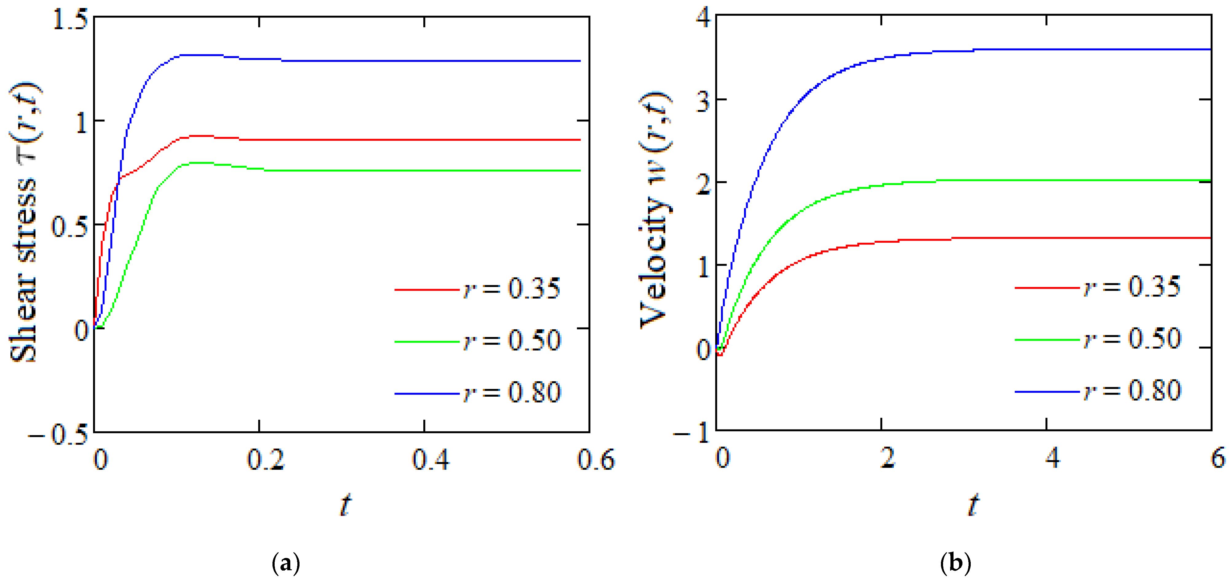
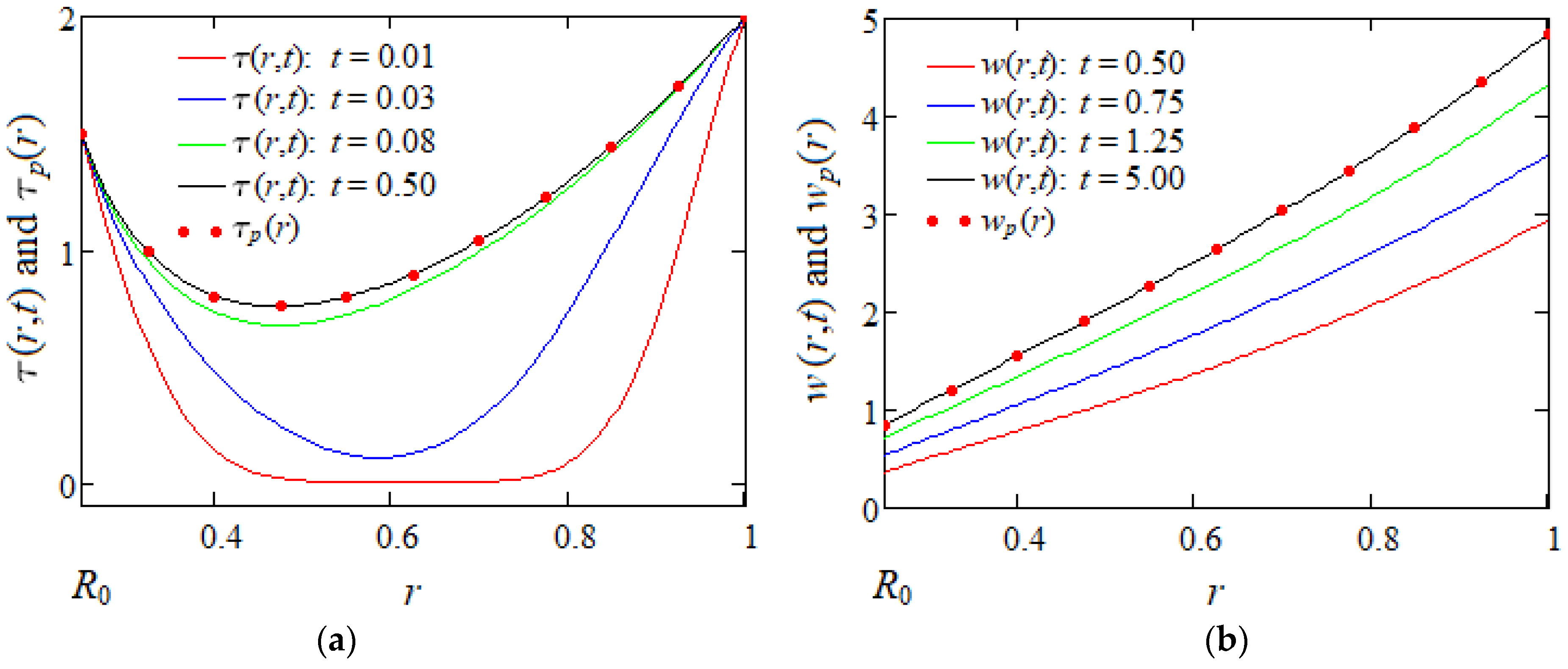
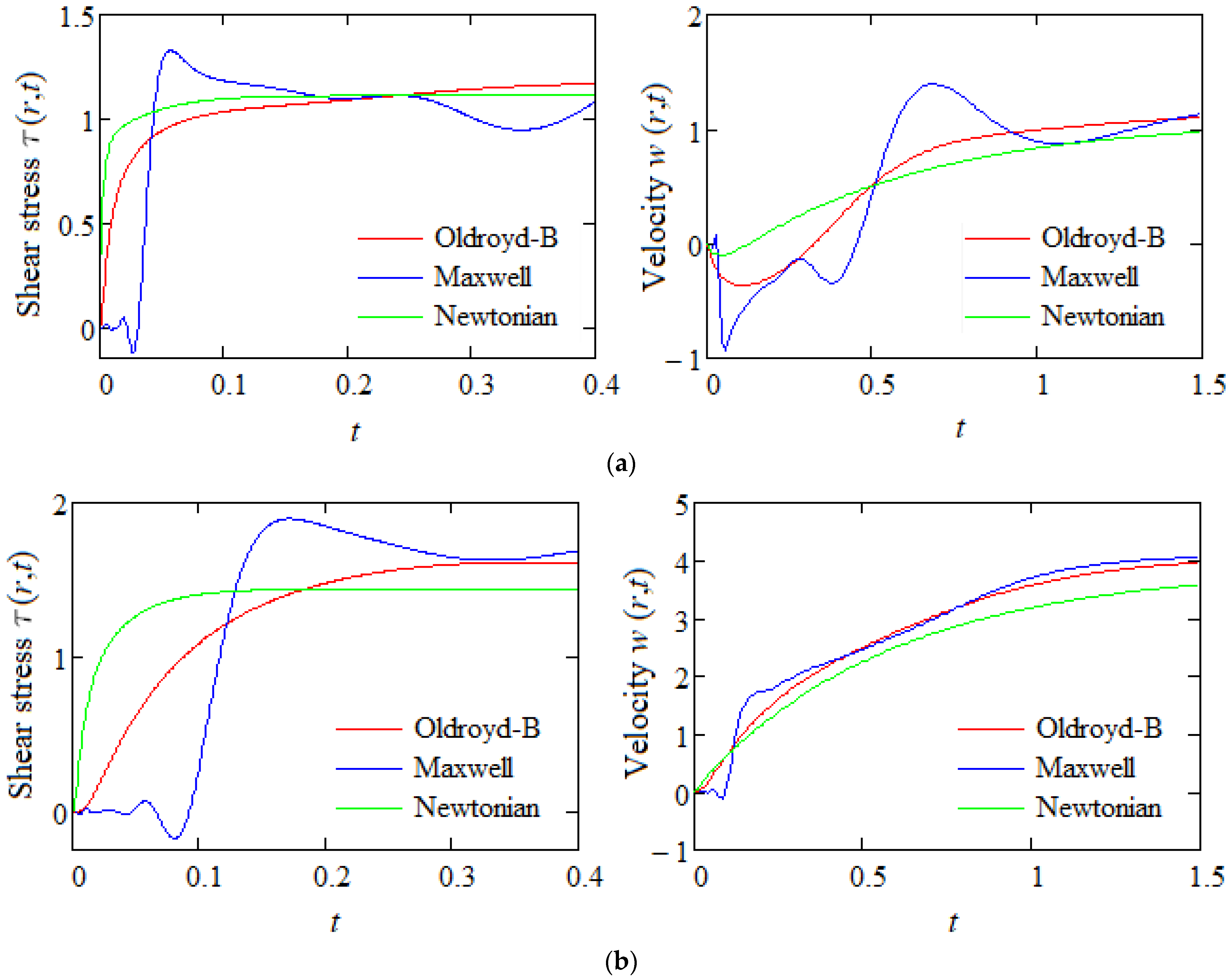
5. Some Numerical Results

In the previous sections, the MHD Taylor–Couette flows of incompressible Oldroyd-B fluids through a porous medium between two infinite coaxial circular cylinders that applies time-dependent couples to the fluid and in an infinite circular cylinder that applies a time-dependent couple to the fluid were studied. Analytical expressions were established for the dimensionless shear stresses, the velocity fields of fluid and Darcy’s resistances by means of the integral transforms. The obtained results, which satisfy all imposed initial and boundary conditions, can be used to give exact solutions for any motion of this type of the respective fluids. Consequently, the motion problems that were considered here are completely solved. In addition, in both cases, similar solutions for MHD Taylor–Couette flows of incompressible Maxwell fluids are immediately obtained taking $b=0$ in the general solutions.

Now, in order to highlight some physical aspects of the MHD flow of incompressible Oldroyd-B fluids in the porous annular domain, we analyzed, by the graphical representations in Figure 2, Figure 3, Figure 4, Figure 5 and Figure 6, a particular case with constant shear stresses on the flow domain’s boundaries. More precisely, we chose the two functions $h(\cdot )$ and $f(\cdot )$ to be $1.5H(t)$ and $2H(t)$, respectively. Here, $H(\cdot )$ is the Heaviside unit step function. The variations in time of the dimensionless shear stress $\tau (r,t)$ and of the fluid velocity $w(r,t)$ in three radial positions of the flow domain are presented in Figure 2.

From Figure 2, it is clearly found that significant variations in the two physical entities appear only for small values of dimensionless time t. After this, they have constant values up to infinity. Consequently, the respective motion becomes steady or permanent in time and the permanent solutions have to be determined. These solutions will be determined using an important property of the Laplace transform, namely, “if $\widehat{g}(s)$ is the Laplace transform of the function $g(t)$ then $\underset{s\to \infty }{\lim } g(t)=\underset{s\to 0}{\lim } s\widehat{g}(s)$”.

Substituting functions $\widehat{h}(s)$ and $\widehat{f}(s)$ by $1.5/s$ and $2/s$, respectively, in Equation (30), applying the inverse finite Hankel transform to the obtained result and using the above mentioned property of the Laplace transform, one finds the following expression

$$\begin{array}{l}{\tau }_p(r)={\displaystyle \frac{1.5(r^4-1)R_0^2}{(R_0^2-1)r^2}}+{\displaystyle \frac{2(R_0^4-r^4)}{(R_0^2-1)r^2}}\\ -\pi {\displaystyle \sum _{n=1}^{\infty }\frac{J_2(r_n)[2J_2(R_0{r}_n)-1.5J_2(r_n)]B_{22}(r,r_n)}{{[J_2(R_0{r}_n)]}^2-{[J_2(r_n)]}^2}}{\displaystyle \frac{K_{eff}}{r_n^2+K_{eff}}},\end{array}$$

(69)

for the dimensionless permanent shear stress ${\tau }_p(r)$. The corresponding expression for the permanent velocity field $w_p(r)$, namely,

$$\begin{array}{l}{w}_p(r)={\displaystyle \frac{1}{2(R_0^4-1)}}\left[1.5\left(r^3+{\displaystyle \frac{1}{r}}\right)R_0^2-2\left(r^3+{\displaystyle \frac{R_0^4}{r}}\right)\right]+{\displaystyle \frac{4r(1.5R_0^2-2)}{(R_0^4-1)K_{eff}}}\\ +{\displaystyle \frac{r[2R_0^2-1.5(R_0^4+1)/2]}{R_0^4-1}}+{\displaystyle \frac{2r}{R_0^2}}{\displaystyle \sum _{n=1}^{\infty }\frac{J_2(r_n)[2J_2(R_0{r}_n)-1.5J_2(r_n)]}{r_n^2{[J_2(R_0{r}_n)]}^2-{[J_2(r_n)]}^2}}\\ -\pi {\displaystyle \sum _{n=1}^{\infty }\frac{J_2(r_n)[2J_2(R_0{r}_n)-1.5J_2(r_n)]B_{21}(r,r_n)}{r_n{[J_2(R_0{r}_n)]}^2-{[J_2(r_n)]}^2}}{\displaystyle \frac{K_{eff}}{r_n^2+K_{eff}}},\end{array}$$

(70)

was obtained using relation (49). The expressions (69) and (70) of ${\tau }_p(r)$ and $w_p(r)$ correspond to both incompressible Newtonian and non-Newtonian fluids. This is not a surprise because the governing equations for the steady motions of these fluids are identical. Moreover, they do not depend on the parameters M and K independently, but only on a combination of them, which is the effective permeability $K_{eff}=M+K$. Consequently, a two-parameter approach in such motions is superfluous.

Of course, the permanent components ${\tau }_{0p}(r)$ and $w_{0p}(r)$ of ${\tau }_0(r,t)$ and $w_0(r,t)$, respectively, can also be determined in the same way as before using relations (60) and (66). Their expressions are given by the relations (see entry 1 of Table X from reference [27]):

$${\tau }_{0p}(r)=2r^2+4{\displaystyle \sum _{n=1}^{\infty }\frac{J_2(r{r}_{0n})}{r_{0n}{J}_1(r_{0n})}}{\displaystyle \frac{K_{eff}}{r_{0n}^2+K_{eff}}}=-4{\displaystyle \sum _{n=1}^{\infty }\frac{r_{0n}{J}_2(r{r}_{0n})}{J_1(r_{0n})}}{\displaystyle \frac{1}{r_{0n}^2+K_{eff}}};\hspace{0.17em}\hspace{0.17em}\hspace{0.17em}0<r<1,$$

(71)

$$w_{0p}(r)={\displaystyle \frac{8r}{K_{eff}}}+4{\displaystyle \sum _{n=1}^{\infty }\frac{J_1(r{r}_{0n})}{J_1(r_{0n})}}{\displaystyle \frac{1}{r_{0n}^2+K_{eff}}};\hspace{0.17em}\hspace{0.17em}\hspace{0.17em}0<r<1.$$

(72)

They also depend on M and K only by means of effective permeability $K_{eff}=M+K$. In addition, simple computations show that ${\tau }_{0p}(r)$ and $w_{0p}(r)$ satisfy the corresponding governing equation obtained from Equation (12) when $a=b=0$.

Now, in order to determine the required time to reach the steady or permanent state and to validate the correctness of the obtained solutions, Figure 3 and Figure 4 show the convergence of the starting shear stresses $\tau (r,t)$, ${\tau }_0(r,t)$ and of the corresponding velocities $w(r,t)$, $w_0(r,t)$ given by relations (35), (62) and (53), (67), respectively, to their permanent components ${\tau }_p(r)$, ${\tau }_{0p}(r)$ and $w_p(r)$, $w_{0p}(r)$ for increasing values of time t. From these figures, it is found that the necessary time to reach the steady state is much smaller for shear stresses in comparison with the fluid velocities. In addition, the boundary conditions are clearly satisfied and, as expected, the fluid velocity is an increasing function with respect to time t. The shear stress is also an increasing function with regard to time t but only for the motion between infinite coaxial cylinders.

Figure 5 were drawn to show the time evolutions of the shear stresses and velocities corresponding to the three types of fluids: Oldroyd-B, Maxwell and Newtonian. In this way, the behavior of the Oldroyd-B fluid is brought to light in comparison with that of Maxwell and Newtonian fluids, which is obtained from the Oldroyd-B model by making the retardation time $b=0$, respectively, the relaxation time $a=0$ and the retardation time $b=0$. The comparison is made in two radial positions of the flow domain $r=0.35$ and $r=0.85$. It is observed from this Figure that the shear stress corresponding to the Maxwell fluid has oscillatory values for small values of time t, while the shear stress corresponding to the Oldroyd-B fluid does not show such oscillations. This is due to the presence of the retardation phenomenon, which delays the elastic response of the fluid. Obviously, for large values of time t, the shear stress values tend towards the values of the permanent solutions.

Figure 6 shows the influence of dimensionless relaxation and retardation times a and b on the dimensionless starting shear stress $\tau (r,t)$ corresponding to the flow between cylinders. From this figure, it is clearly seen that the boundary conditions are satisfied and, as expected, the shear stress is an increasing function with respect to the relaxation time a and a decreasing one with regard to the retardation time b. It declines from a maximum value on the inner cylinder up to an absolute minimum value in its vicinity and then continues to increase up to a new maximum value on the exterior cylinder.

6. Conclusions

The Taylor–Couette flow of incompressible Oldroyd-B fluids between two infinite coaxial circular cylinders that apply time-dependent couples to the fluid has been analytically investigated under the influence of a magnetic field and a porous medium. Similar solutions for the Taylor–Couette flow of same fluids through an infinite circular cylinder that applies a time-dependent couple to the fluid have been obtained as limiting cases of previous results. The solutions obtained were used to bring to light some characteristics of the fluid motion and to find the necessary time to reach the permanent or steady state.

-

The main outcomes that have been obtained by this study are:

-

The Taylor–Couette flow of ECIOBFs through a porous medium induced by time-dependent couples in an annulus was investigated in the presence of a magnetic field.

-

Closed-form expressions are established for the dimensionless shear stress and fluid velocity. A particular case is considered and the steady solutions are also provided.

-

The solutions for a Taylor–Couette flow of same fluids induced by time-dependent couple in an infinite circular cylinder were obtained as limiting cases of previous results.

-

The convergence of starting solutions to their steady components was graphically proven and the necessary times to touch the permanent state were found.

-

The permanent solutions, which are the same for flows of incompressible Newtonian and non-Newtonian fluids, do not depend on parameters M and K independently and a two-parameter approach is superfluous.

To the best of our knowledge, the exact solutions for MHD unsteady motions of incompressible Burgers fluids through a porous medium in cylindrical domains are lacking in the existing literature. Consequently, similar motions of these fluids induced by two infinite coaxial circular cylinders that slide along their common symmetry axis or rotate around the same axis could be investigated.

References

1. Waters, N.D.; King, M.J. The unsteady flow of an elastico-viscous liquid in a straight pipe of circular cross section. J. Phys. D Appl. Phys. 1971, 4, 204–211. [Google Scholar] [CrossRef]
2. Rajagopal, K.R.; Bhatnagar, R.K. Exact solutions for simple flows of an Oldroyd-B fluid. Acta Mech. 1995, 113, 233–239. [Google Scholar] [CrossRef]
3. Wood, W.P. Transient viscoelastic helical flow in pipes of circular and annular cross-section. J. Non-Newton. Fluid Mech. 2001, 100, 115–126. [Google Scholar] [CrossRef]
4. Fetecau, C. Analytical solutions for non-Newtonian fluid flows in pipe-like domains. Int. J. Non-Linear Mech. 2004, 39, 225–231. [Google Scholar] [CrossRef]
5. McGinty, S.; McKee, S.; McDermott, R. Analytic solutions of Newtonian and non-Newtonian pipe flows subject to a general time-dependent pressure gradient. J. Non-Newton. Fluid Mech. 2009, 162, 54–77. [Google Scholar] [CrossRef]
6. Fetecau, C.; Imran, M.; Fetecau, C. Taylor-Couette flow of an Oldroyd-B fluid in an annulus due to a time-dependent couple. Z. Naturforschung A 2011, 66, 40–46. [Google Scholar] [CrossRef]
7. Jamil, M.; Khan, N.A. Axial Couette flow of an Oldroyd-B fluid in an annulus. Theor. Appl. Mech. Lett. 2012, 2, 012001. [Google Scholar] [CrossRef]
8. Imran, M.; Tahir, M.; Imran, M.A.; Awan, A.U. Taylor-Couette flow of an Oldroyd-B fluid in an annulus subject to a time dependent rotation. Am. J. Appl. Math. 2015, 3, 25–31. [Google Scholar] [CrossRef]
9. Ullah, S.; Tanveer, M.; Bajwa, S. Study of velocity and shear stress for unsteady flow of incompressible Oldroyd-B fluid between two concentric rotating circular cylinders. Hacet. J. Math. Stat. 2019, 48, 372–383. [Google Scholar] [CrossRef]
10. Khan, M.; Malik, R.; Anjun, A. Analytic solutions for MHD flows of an Oldroyd-B fluid between two side walls perpendicular to the plate. Chem. Eng. Commun. 2011, 198, 1415–1434. [Google Scholar] [CrossRef]
11. Zahid, M.; Rana, M.A.; Haroon, T.; Siddiqui, A.M. Applications of Sumudu transform to MHD flows of an Oldroyd-B fluid. Appl. Math. Sci. 2013, 7, 7027–7036. [Google Scholar] [CrossRef]
12. Ghosh, A.K.; Datta, S.K.; Sen, P. On hydromagnetic flow of an Oldroyd-B fluid between two oscillating plates. Int. J. Appl. Comput. Math. 2016, 2, 365–386. [Google Scholar] [CrossRef]
13. Tan, W.C.; Masuoka, T. Stokes’ first problem for an Oldroyd-B fluid in a porous medium. Phys. Fluids 2005, 17, 023101. [Google Scholar] [CrossRef]
14. Khan, I.; Imran, M.; Fakhar, K. New exact solutions for an Oldroyd-B fluid in a porous medium. Int. J. Math. Math. Sci. 2011, 2011, 408132. [Google Scholar] [CrossRef]
15. Hayat, T.; Shehzad, S.A.; Mustafa, M.; Hendi, A. MHD flow of an Oldroyd-B fluid through a porous channel. Int. J. Chem. React. Eng. 2012, 10, Article ID A8. [Google Scholar] [CrossRef]
16. Sultan, Q.; Nazar, M.; Ali, U.; Imran, M. Unsteady flow of Oldroyd-B fluid through porous rectangular duct. Int. J. Nonlinear Sci. 2013, 15, 195–211. [Google Scholar]
17. Khan, I.; Ijaz, A. Starting solutions for an MHD Oldroyd-B fluid through porous space. J. Porous Media 2014, 17, 797–809. [Google Scholar] [CrossRef]
18. Hayat, T.; Hussain, M.; Khan, M. Hall effect on flows of an Oldroyd-B fluid through porous medium for cylindrical geometries. Comput. Math. Appl. 2006, 52, 269–282. [Google Scholar] [CrossRef]
19. Hamza, S.E.E. MHD flow of an Oldroyd-B fluid through porous medium in a circular channel under the effect of time dependent pressure gradient. Am. J. Fluid Dyn. 2017, 7, 1–11. [Google Scholar]
20. Riaz, M.B.; Awrejcewicz, J.; Rehman, A.U. Functional effects of permeability on Oldroyd-B fluid under magnetization: A comparison of slipping and non-slipping solutions. Appl. Sci. 2021, 11, 11477. [Google Scholar] [CrossRef]
21. Fetecau, C.; Vieru, D. Investigating Magnetohydrodynamic Motions of Oldroyd-B Fluids through a Circular Cylinder Filled with Porous Medium. Processes 2024, 12, 1354. [Google Scholar] [CrossRef]
22. Fetecau, C.; Vieru, D.; Eva, L.; Forna, N.C. Memory effects in the magnetohydrodynamic axial symmetric flows of Oldroyd-B fluids in a porous annular channel. Symmetry 2024, 16, 1108. [Google Scholar] [CrossRef]
23. Bandelli, R.; Rajagopal, K.R. Start-up flows of second grade fluids in domains with one finite dimension. Int. J. Non-Linear Mech. 1995, 30, 817–839. [Google Scholar] [CrossRef]
24. Oldroyd, J.G. On the formulation of rheological equations of state. Proc. R. Soc. Lond. Ser. A 1950, 200, 523–541. [Google Scholar] [CrossRef]
25. Rossow, V.J. On flow of electrically conducting fluids over a flat plate in the presence of a transverse magnetic field. NACA TN Tech. Rep. 1957, 3971, 489–508. [Google Scholar]
26. Debnath, L.; Bhatta, D. Integral Transforms and Their Applications, 2nd ed.; Cgapman & Hall/CRC: Boca Raton, FL, USA, 2007. [Google Scholar]
27. Sneddon, I.N. Fourier Transforms; McGraw-Hill Book Company, Inc.: New York, NY, USA; Toronto, ON, Canada; London, UK, 1951. [Google Scholar]
Figure 1. Geometry of the flow.
Mathematics 13 00719 g001
Figure 2. (a) Shear stress  τ ( r , t ) ; (b) velocity  w ( r , t ) . Variations in time of shear stress  τ ( r , t )  and velocity  w ( r , t )  given by Equations (35) and (53) for  R 0 = 0.25 , M = 1 , K = 0.7 , a = 0.025 , b = 0.010  and increasing values of r.
Mathematics 13 00719 g002
Figure 3. (a) Shear stress  τ ( r , t )  and  τ p ( r ) ; (b) velocity  w ( r , t )  and  w p ( r ) . Convergence of  τ ( r , t )  and  w ( r , t )  given by Equations (35) and (53) to their permanent components  τ p ( r ) w p ( r )  from Equations (69) and (70) when  M = 1 , K = 0.7 , a = 0.025 , b = 0.010 ,   R 0 = 0.25  and increasing values of the time t.
Mathematics 13 00719 g003
Figure 4. (a) Shear stress  τ 0 ( r , t )  and  τ 0 p ( r ) ; (b) velocity  w 0 ( r , t )  and  w 0 p ( r ) . Convergence of  τ 0 ( r , t )  and  w 0 ( r , t )  given by Equations (62) and (67) to their permanent components  τ 0 p ( r ) w 0 p ( r )  from Equations (71) and (72) when  M = 0.75 , K = 1.2 , a = 0.025 ,   b = 0.010  and increasing values of the time t.
Mathematics 13 00719 g004
Figure 5. (a r = 0.3 ; (b r = 0.85 . Comparisons of shear stress  τ ( r , t )  and velocity  w ( r , t )  given by Equations (35) and (53) corresponding to Oldroyd-B, Maxwell and Newtonian fluids for  R 0 = 0.25 , r = 0.3  and  r = 0.85 ,  M = 1 , K = 0.7  and  a = 0.6 , b = 0.1  (Oldroyd-B),  a = 0.6 , b = 0  (Maxwell),  a = b = 0  (Newtonian).
Mathematics 13 00719 g005
Figure 6. (a) Shear stress  τ ( r , t )  depending of a; (b) shear stress  τ ( r , t )  depending of b. Variations in the shear stress  τ ( r , t )  given by Equation (35) with the relaxation a and retardation b times when  R 0 = 0.25 , M = 1 , K = 0.7 , t = 0.4 .
Mathematics 13 00719 g006
Disclaimer/Publisher’s Note: The statements, opinions and data contained in all publications are solely those of the individual author(s) and contributor(s) and not of MDPI and/or the editor(s). MDPI and/or the editor(s) disclaim responsibility for any injury to people or property resulting from any ideas, methods, instructions or products referred to in the content.