
A Particle Swarm Optimization-Based Ensemble Broad Learning System for Intelligent Fault Diagnosis in Safety-Critical Energy Systems with High-Dimensional Small Samples

Abstract
1. Introduction
1.1. Problem Statement
1.2. Research Motivation
1.3. Research Gap
1.4. Contribution Statement
- (1)
- This paper introduces a novel IFD approach for SCESs, where the BLS method is employed as an alternative to deep learning techniques for fault diagnosis.
- (2)
- We propose an EBLS framework that integrates the random forest(RF)algorithm and an ensemble strategy into the traditional BLS model, designed to handle high-dimensional small samples for improved stability and classification accuracy.
- (3)
- The PSO algorithm is utilized to optimize the hyperparameters of the EBLS framework, leading to reduced computational costs and improved performance.
2. Preliminaries
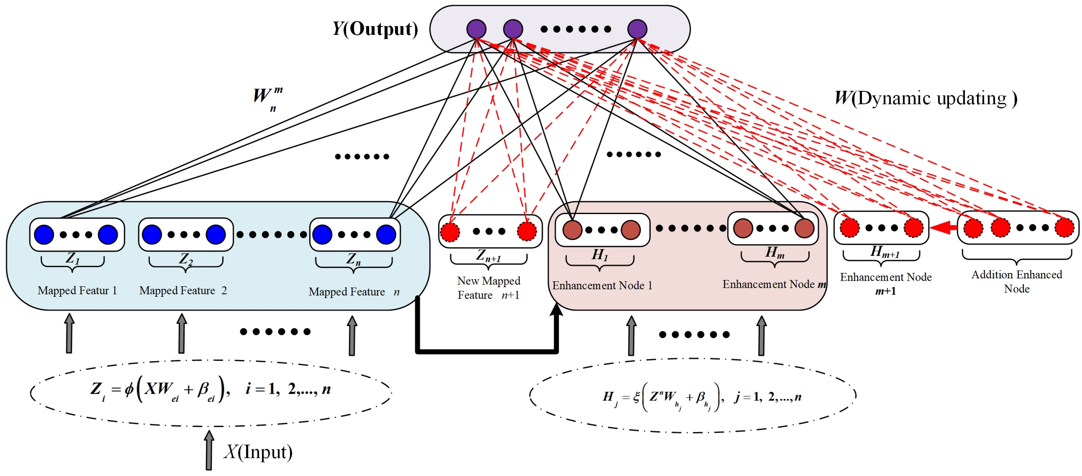
2.1. BLS
2.2. RF
2.3. PSO
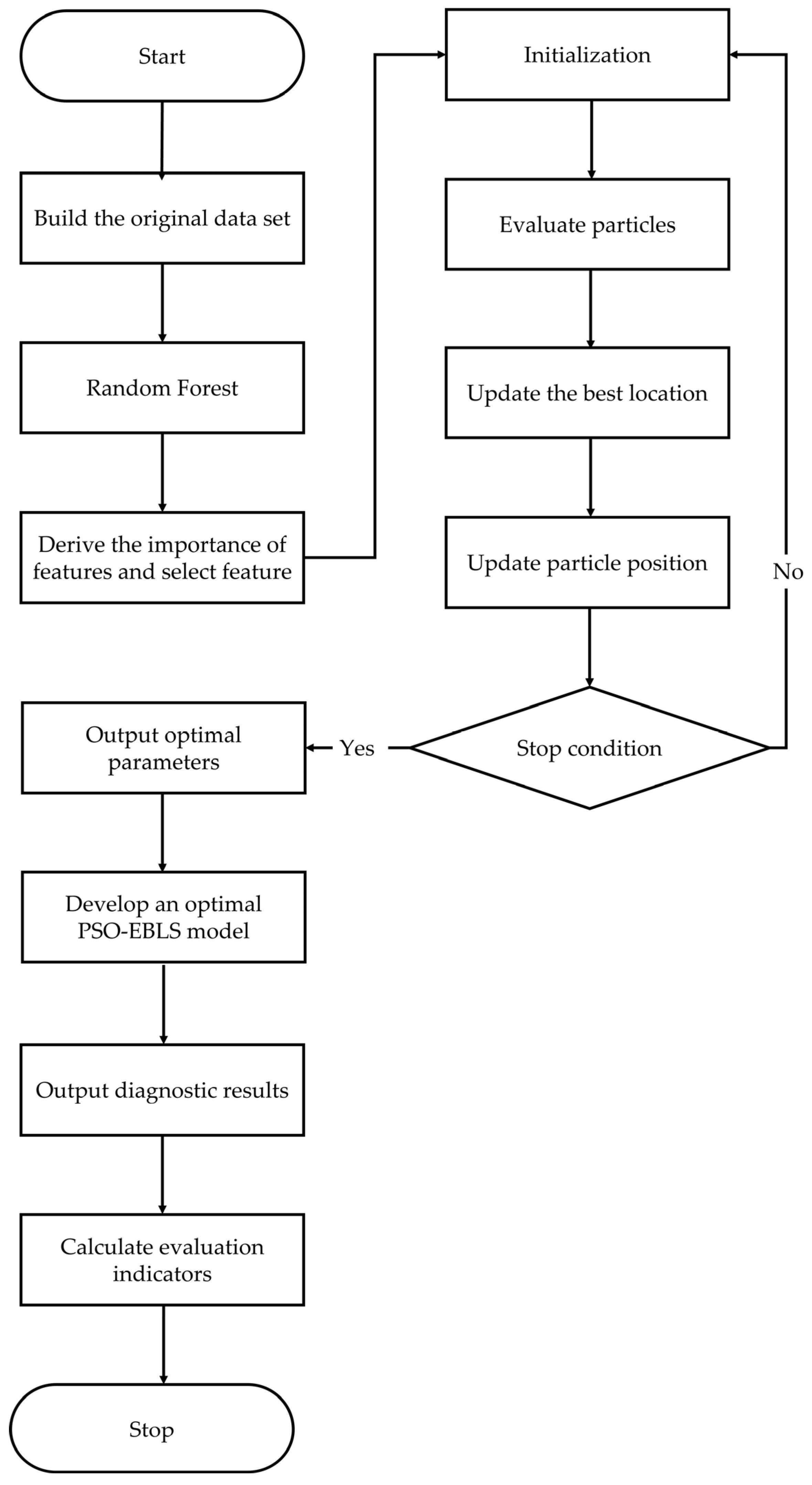
3. Materials and Methods
3.1. Definitions of EBLS Methods
- (1)
- Feature selection: Multiple factors are associated with fault occurrence in SCESs; however, certain faults may have less relevance, which can reduce the model’s learning capability. Given that many features are independent of one another, we apply a RF feature selection strategy to automatically identify and filter the most relevant features.
- (2)
- Establish sub-training datasets: The entire dataset is split into two subsets: a training dataset (of size ) and a test dataset (of size ). samples are chosen from the training dataset using the Bootstrapping technique where is the sampling ratio, and represents the largest integer no more than . This sampling process is repeated times to prepare different sub-training datasets for training the sub-models.
- (3)
- Build the EBLS models: In this model, each EBLS model is regarded as a weak learner in the ensemble learning model. Then, we combine multiple weak learners to form strong learners. Finally, the output of the EBLS model can be computed bywhere is the predicted value of the learner, while is final predicted value.
3.2. Definitions of the PSO-EBLS Methods
4. Experimental Results and Analysis
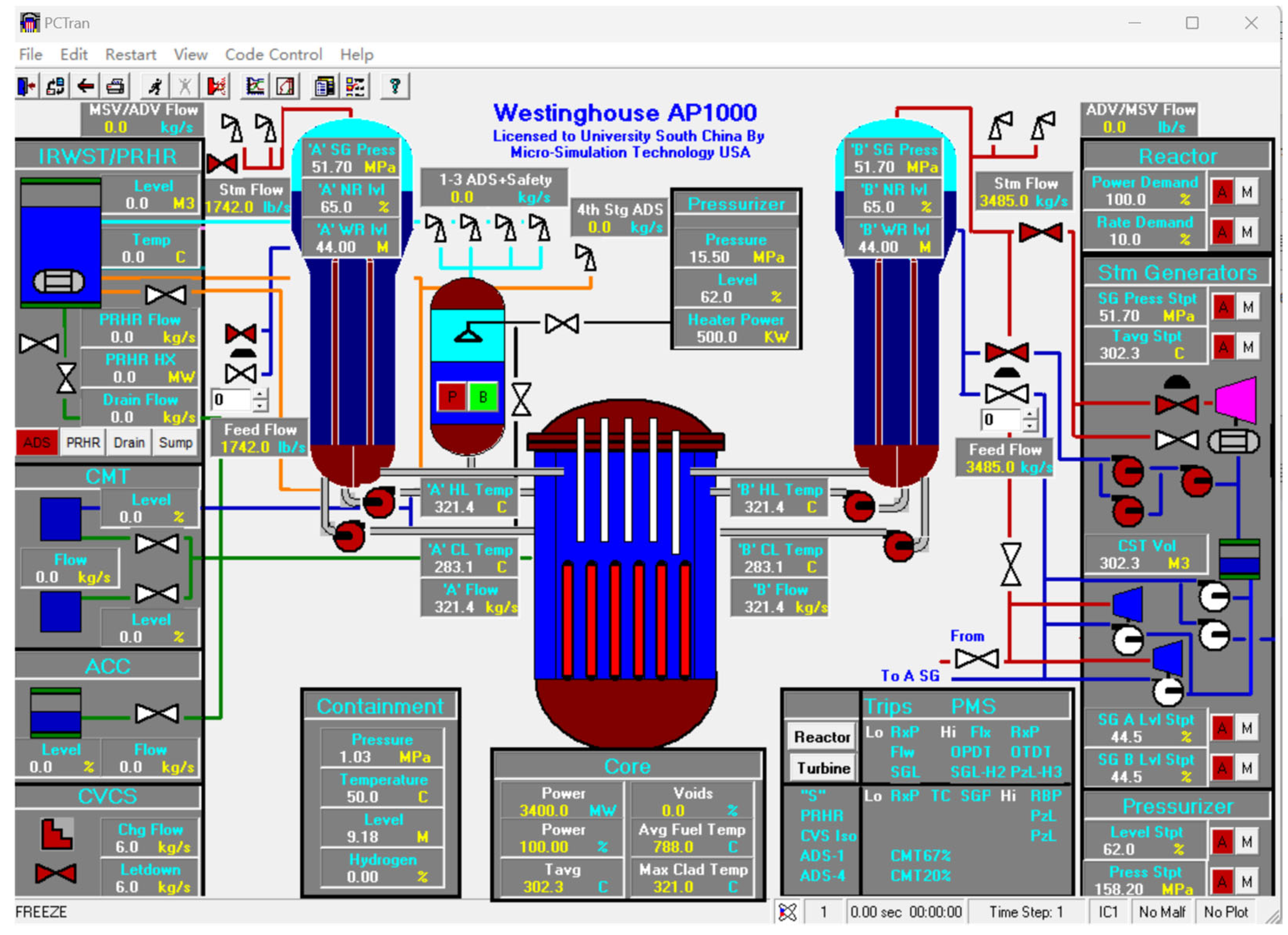
4.1. Experiment Data and Environment
4.1.1. Experiment Data
- (1)
- Nature of the Samples:
- (a)
- NO (L1): Represents operational data under normal conditions, including steady-state parameters such as coolant temperature, pressure, and flow rate.
- (b)
- SBLOCA (L2): Represents operational data under partial pipe ruptures with equivalent diameters ranging from 9.5 mm to 25.0 mm. Such accidents result in a gradual coolant leakage, leading to a decrease in both the NRCS pressure and the water level in the pressurizer over time. This gradual loss can also cause an increase in containment temperature and pressure due to heat release at the rupture site.
- (c)
- LBLOCA (L3): Represents operational data under severe pipe ruptures with equivalent diameters greater than 34.5 mm. This type of accident leads to rapid coolant loss, resulting in abrupt changes in system pressure and temperature.
- (d)
- SGTR (L4): Represents operational data related to the failure caused by the rupture of one or more U-tubes in the steam generator. Following a SGTR, coolant from the primary loop leaks into the secondary loop, leading to a gradual increase in the radioactive level within the secondary loop. Concurrently, the pressure in the primary loop and the pressurizer water level decrease, while the pressure in the secondary loop rises.
- (e)
- LOFA (L5): Represents operational data during a coolant flow loss event caused by a main pump failure or shutdown. This results in a decrease in coolant flow, an increase in reactor coolant temperature and pressure, and a rise in pressurizer level.
- (2)
- Sample Collection Methodology:
- The samples were generated using PCTRAN, and the steps are as follows:
- (a)
- Simulated Operational Environment: The simulator was configured with operational parameters that mirror real-world NRCS, including a total of 85 fault characteristics.
- (b)
- Data Acquisition: Time series data were collected at regular intervals under different operational and accident scenarios.
- (c)
- Fault Labeling: Based on predefined fault scenarios, the data were labeled into specific categories (L1–L5).
4.1.2. Experiment Environment
4.2. Comparison and Analysis of the Diagnostic Results
4.2.1. Evaluation Metrics
4.2.2. Diagnostic Results
4.2.3. Comparison and Analysis
5. Conclusions
Author Contributions
Funding
Data Availability Statement
Acknowledgments
Conflicts of Interest
References
- Süle, Z.; Baumgartner, J.; Dörgő, G.; Abonyi, J. P-graph-based multi-objective risk analysis and redundancy allocation in safety-critical energy systems. J. Energy 2019, 179, 989–1003. [Google Scholar] [CrossRef]
- Yao, Y.; Han, T.; Yu, J.; Xie, M. Uncertainty-aware deep learning for reliable health monitoring in safety-critical energy systems. J. Energy 2024, 291, 130419. [Google Scholar] [CrossRef]
- Meng, L.; Asuka, J. Impacts of energy transition on life cycle carbon emission and water consumption in Japan’s electric sector. J. Sustain. 2022, 14, 5413. [Google Scholar] [CrossRef]
- Gao, Z.; Cecati, C.; Ding, S.X. A survey of fault diagnosis and fault-tolerant techniques—Part I: Fault diagnosis with model-based and signal-based approaches. J. IEEE Trans. Ind. Electron. 2015, 62, 3757–3767. [Google Scholar] [CrossRef]
- Li, J.; Lin, M. Research on robustness of five typical data-driven fault diagnosis models for nuclear power plants. J. Ann. Nucl. Energy 2022, 165, 108639. [Google Scholar] [CrossRef]
- Guo, H.; Hu, S.; Wang, F.; Zhang, L. A novel method for quantitative fault diagnosis of photovoltaic systems based on data-driven. J. Electr. Power Syst. Res. 2022, 210, 108121. [Google Scholar] [CrossRef]
- Lei, Y.; Yang, B.; Jiang, X.; Jia, F.; Li, N.; Nandi, A.K. Applications of machine learning to machine fault diagnosis: A review and roadmap. J. Mech. Syst. Signal Process. 2020, 138, 106587. [Google Scholar] [CrossRef]
- Chen, Z.; Chen, J.; Liu, S.; Feng, Y.; He, S.; Xu, E. Multi-channel Calibrated Transformer with Shifted Windows for few-shot fault diagnosis under sharp speed variation. J. ISA Trans. 2022, 131, 501–515. [Google Scholar] [CrossRef] [PubMed]
- Zhang, T.; Chen, J.; Li, F.; Zhang, K.; Lv, H.; He, S.; Xu, E. Intelligent fault diagnosis of machines with small & imbalanced data: A state-of-the-art review and possible extensions. J. ISA Trans. 2022, 119, 152–171. [Google Scholar] [CrossRef]
- Khentout, N.; Magrotti, G. Fault supervision of nuclear research reactor systems using artificial neural networks: A review with results. J. Ann. Nucl. Energy 2023, 185, 109684. [Google Scholar] [CrossRef]
- Atoui, M.A.; Cohen, A. Coupling data-driven and model-based methods to improve fault diagnosis. J. Comput. Ind. 2021, 128, 103401. [Google Scholar] [CrossRef]
- Irani, F.N.; Soleimani, M.; Yadegar, M.; Meskin, N. Deep transfer learning strategy in intelligent fault diagnosis of gas turbines based on the Koopman operator. J. Appl. Energy 2024, 365, 123256. [Google Scholar] [CrossRef]
- Jiang, F.; Chen, J.; Rong, J.; Liu, W.; Li, H.; Peng, H. Safe reinforcement learning based optimal low-carbon scheduling strategy for multi-energy system. J. Sustain. Energy Grids Netw. 2024, 39, 101454. [Google Scholar] [CrossRef]
- Fang, W.; Zhou, B.; Zhang, Y.; Yu, X.; Jiang, S.; Wei, J. A Fault Diagnosis and Fault-Tolerant Control Method for Current Sensors in Doubly Salient Electromagnetic Motor Drive Systems. J. IEEE J. Emerg. Sel. Top. Power Electron. 2024, 12, 2234–2248. [Google Scholar] [CrossRef]
- Zhang, J.; Zhang, K.; An, Y.; Luo, H.; Yin, S. An integrated multitasking intelligent bearing fault diagnosis scheme based on representation learning under imbalanced sample condition. J. IEEE Trans. Neural Netw. Learn. Syst. 2023, 35, 6231–6242. [Google Scholar] [CrossRef]
- Zheng, Y.; Wang, D. An Auxiliary Classifier Generative Adversarial Network based Fault Diagnosis for Analog Circuit. J. IEEE Access 2023, 11, 86824–86833. [Google Scholar] [CrossRef]
- Jieyang, P.; Kimmig, A.; Dongkun, W.; Niu, Z.; Zhi, F.; Jiahai, W.; Liu, X.; Ovtcharova, J. A systematic review of data-driven approaches to fault diagnosis and early warning. J. J. Intell. Manuf. 2023, 34, 3277–3304. [Google Scholar] [CrossRef]
- Abid, A.; Khan, M.T.; Iqbal, J. A review on fault detection and diagnosis techniques: Basics and beyond. J. Artif. Intell. Rev. 2021, 54, 3639–3664. [Google Scholar] [CrossRef]
- Li, G.; Chen, L.; Fan, C.; Li, T.; Xu, C.; Fang, X. Interpretation and explanation of convolutional neural network-based fault diagnosis model at the feature-level for building energy systems. J. Energy Build. 2023, 295, 113326. [Google Scholar] [CrossRef]
- Zhu, S.; Xia, H.; Annor-Nyarko, M.; Yin, W.; Peng, B.; Wang, Z.; Zhang, J. A robust strategy for sensor fault detection in nuclear power plants based on principal component analysis. J. Ann. Nucl. Energy 2021, 164, 108621. [Google Scholar] [CrossRef]
- Zhang, C.; Tian, X.; Zhao, Y.; Li, T.; Zhou, Y.; Zhang, X. Causal discovery-based external attention in neural networks for accurate and reliable fault detection and diagnosis of building energy systems. J. Build. Environ. 2022, 222, 109357. [Google Scholar] [CrossRef]
- Amiri, A.F.; Oudira, H.; Chouder, A.; Kichou, S. Faults detection and diagnosis of PV systems based on machine learning approach using random forest classifier. J. Energy Convers. Manag. 2024, 301, 118076. [Google Scholar] [CrossRef]
- Et-taleby, A.; Chaibi, Y.; Boussetta, M.; Allouhi, A.; Benslimane, M. A novel fault detection technique for PV systems based on the K-means algorithm, coded wireless Orthogonal Frequency Division Multiplexing and thermal image processing techniques. J. Sol. Energy 2022, 237, 365–376. [Google Scholar] [CrossRef]
- Tuerxun, W.; Chang, X.; Hongyu, G.; Zhijie, J.; Huajian, Z. Fault diagnosis of wind turbines based on a support vector machine optimized by the sparrow search algorithm. J. IEEE Access 2021, 9, 69307–69315. [Google Scholar] [CrossRef]
- Mansouri, M.; Fezai, R.; Trabelsi, M.; Hajji, M.; Harkat, M.F.; Nounou, H.; Nounou, M.; Bouzrara, K. A novel fault diagnosis of uncertain systems based on interval gaussian process regression: Application to wind energy conversion systems. J. IEEE Access 2020, 8, 219672–219679. [Google Scholar] [CrossRef]
- De Santis, E.; Rizzi, A. Modeling failures in smart grids by a bilinear logistic regression approach. J. Neural Netw. 2024, 174, 106245. [Google Scholar] [CrossRef]
- Qiu, S.; Cui, X.; Ping, Z.; Shan, N.; Li, Z.; Bao, X.; Xu, X. Deep learning techniques in intelligent fault diagnosis and prognosis for industrial systems: A review. J. Sens. 2023, 23, 1305. [Google Scholar] [CrossRef] [PubMed]
- Du, Z.; Chen, S.; Li, P.; Chen, K.; Liang, X.; Zhu, X.; Jin, X. Knowledge-extracted deep learning diagnosis and its cloud-based management for multiple faults of chiller. J. Build. Environ. 2023, 235, 110228. [Google Scholar] [CrossRef]
- Seghiour, A.; Abbas, H.A.; Chouder, A.; Rabhi, A. Deep learning method based on autoencoder neural network applied to faults detection and diagnosis of photovoltaic system. J. Simul. Model. Pract. Theory 2023, 123, 102704. [Google Scholar] [CrossRef]
- Harrou, F.; Dairi, A.; Taghezouit, B.; Khaldi, B.; Sun, Y. Automatic fault detection in grid-connected photovoltaic systems via variational autoencoder-based monitoring. J. Energy Convers. Manag. 2024, 314, 118665. [Google Scholar] [CrossRef]
- Gong, X.; Zhang, T.; Chen, C.P.; Liu, Z. Research review for broad learning system: Algorithms, theory, and applications. J. IEEE Trans. Cybern. 2021, 52, 8922–8950. [Google Scholar] [CrossRef]
- Wang, X.; Wang, C.; Zhu, K.; Zhao, X. A Mechanical Equipment Fault Diagnosis Model Based on TSK Fuzzy Broad Learning System. J. Symmetry 2022, 15, 83. [Google Scholar] [CrossRef]
- Chen, C.P.; Liu, Z.; Feng, S. Universal approximation capability of broad learning system and its structural variations. J. IEEE Trans. Neural Netw. Learn. Syst. 2018, 30, 1191–1204. [Google Scholar] [CrossRef] [PubMed]
- Yang, K.; Yu, Z.; Chen, C.P.; Cao, W.; You, J.; Wong, H.S. Incremental weighted ensemble broad learning system for imbalanced data. J. IEEE Trans. Knowl. Data Eng. 2021, 34, 5809–5824. [Google Scholar] [CrossRef]
- Li, K.; Wang, F.; Yang, L.; Liu, R. Deep feature screening: Feature selection for ultra high-dimensional data via deep neural networks. J. Neurocomputing 2023, 538, 126186. [Google Scholar] [CrossRef]
- Pei, W.; Xue, B.; Shang, L.; Zhang, M. Developing interval-based cost-sensitive classifiers by genetic programming for binary high-dimensional unbalanced classification [research frontier]. J. IEEE Comput. Intell. Mag. 2021, 16, 84–98. [Google Scholar] [CrossRef]
- Li, J.; Lin, M.; Li, Y.; Wang, X. Transfer learning network for nuclear power plant fault diagnosis with unlabeled data under varying operating conditions. J. Energy 2022, 254, 124358. [Google Scholar] [CrossRef]
- Li, G.; Yu, Z.; Yang, K.; Chen, C.P.; Li, X. Ensemble-Enhanced Semi-Supervised Learning with Optimized Graph Construction for High-Dimensional Data. J. IEEE Trans. Pattern Anal. Mach. Intell. 2024, 47, 1103–1119. [Google Scholar] [CrossRef] [PubMed]
- Zhao, M.; Ye, N. High-Dimensional Ensemble Learning Classification: An Ensemble Learning Classification Algorithm Based on High-Dimensional Feature Space Reconstruction. J. Appl. Sci. 2024, 14, 1956. [Google Scholar] [CrossRef]
- Zhao, B.; Yang, D.; Karimi, H.R.; Zhou, B.; Feng, S.; Li, G. Filter-wrapper combined feature selection and adaboost-weighted broad learning system for transformer fault diagnosis under imbalanced samples. J. Neurocomputing 2023, 560, 126803. [Google Scholar] [CrossRef]
- Cheng, C.; Wang, W.; Chen, H.; Zhang, B.; Shao, J.; Teng, W. Enhanced fault diagnosis using broad learning for traction systems in high-speed trains. J. IEEE Trans. Power Electron. 2020, 36, 7461–7469. [Google Scholar] [CrossRef]
- Xia, H.; Tang, J.; Yu, W.; Qiao, J. Tree broad learning system for small data modeling. J. IEEE Trans. Neural Netw. Learn. Syst. 2022, 35, 8909–8923. [Google Scholar] [CrossRef] [PubMed]
- Wu, J.; Chen, X.Y.; Zhang, H.; Xiong, L.D.; Lei, H.; Deng, S.H. Hyperparameter optimization for machine learning models based on Bayesian optimization. J. J. Electron. Sci. Technol. 2019, 17, 26–40. [Google Scholar] [CrossRef]
- Viswanathan, S.; Ravichandran, K.S. Gain-based Green Ant Colony Optimization for 3D Path Planning on Remote Sensing Images. J. Spectr. Oper. Res. 2025, 2, 92–113. [Google Scholar] [CrossRef]
- Mzili, T.; Mzili, I.; Riffi, M.E.; Pamucar, D.; Simic, V.; Kurdi, M. A novel discrete rat swarm optimization algorithm for the quadratic assignment problem. J. Facta Univ. Ser. Mech. Eng. 2023, 21, 529–552. [Google Scholar] [CrossRef]
- Mzili, T.; Mzili, I.; Riffi, M.E.; Dragan, P.; Vladimir, S.; Laith, A.; Bandar, A. Hybrid genetic and penguin search optimization algorithm (GA-PSEOA) for efficient flow shop scheduling solutions. J. Facta Univ. Ser. Mech. Eng. 2024, 22, 77–100. [Google Scholar] [CrossRef]
- Zhao, F.; Ji, F.; Xu, T.; Zhu, N. Hierarchical parallel search with automatic parameter configuration for particle swarm optimization. J. Appl. Soft Comput. 2024, 151, 111126. [Google Scholar] [CrossRef]


| No. | Fault Type | Name | Labels | Sample Size | Feature Dimension |
|---|---|---|---|---|---|
| 1 | Normal operating | No | L1 | 100 | 85 |
| 2 | Small-break loss of coolant accident | SBLOCA | L2 | 100 | 85 |
| 3 | Large-break loss of coolant accident | LBLOCA | L3 | 100 | 85 |
| 4 | Steam generator tube rupture accident | SGTR | L4 | 100 | 85 |
| 5 | Loss of flow accident | LOFA | L5 | 100 | 85 |
| No. | Name | Parameter |
|---|---|---|
| 1 | Emulation device | Lenovo Legion R9000P (2023 Edition) (Lenovo, Hong Kong, China) |
| 2 | Central processing unit (CPU) | AMD Ryzen 9 7945HX (AMD, Santa Clara, CA, USA) |
| 3 | Graphics processing unit (GPU) | NVIDIA GeForce RTX4060 (NVIDIA, Santa Clara, CA, USA) |
| 4 | Operating system | Microsoft Windows 11 |
| 5 | Simulation software | MATLAB R2023b |
| Algorithm | Parameter Setting | Value |
|---|---|---|
| CNN | Learning Rate | 0.001 |
| Batch Size | 32 | |
| Number of Filters | 16 | |
| Kernel Size | 3 × 3 | |
| Pooling Size | 2 × 2 | |
| Pooling Stride | 2 | |
| Activation Function | ReLU | |
| Dropout Rate | 0.2 | |
| Epochs | 100 | |
| SVM | Regularization parameter | 0.01 |
| Type of kernel function | Linear | |
| Kernel parameter | 0.001 | |
| Tolerance for optimization | 0.0001 | |
| BLS | Number of feature node windows | 5 |
| Number of nodes in each feature node window | 10 | |
| Number of enhancement nodes | 50 | |
| EBLS | Number of trees | 100 |
| Maximum depth of each tree | 10 | |
| Minimum samples required to be at a leaf node | 8 | |
| Minimum samples required to split an internal node | 2 | |
| PSO-EBLS | Iterations | 100 |
| Population | 8 | |
| Inertia weights | 0.7 | |
| Individual Learning Factor | 2 | |
| Social Learning Factor | 2 | |
| Lower band | [10 10 10] | |
| Upper band | [100 100 100] |
| Model | NO. | |||||
|---|---|---|---|---|---|---|
| 1 (%) | 2 (%) | 3 (%) | 4 (%) | 5 (%) | Average Accuracy (%) | |
| CNN | 92.7 | 93.2 | 93.0 | 93.4 | 93.1 | 93.08 |
| SVM | 78.00 | 88.00 | 90.00 | 86.00 | 90.00 | 86.40 |
| BLS | 94.5 | 97.6 | 93.8 | 96.3 | 95.0 | 95.44 |
| EBLS | 97.2 | 97.5 | 97.3 | 97.6 | 97.4 | 97.40 |
| PSO-EBLS | 98.1 | 98.3 | 98.2 | 98.4 | 98.3 | 98.26 |
| Model | NO. | |||||
|---|---|---|---|---|---|---|
| 1 (%) | 2 (%) | 3 (%) | 4 (%) | 5 (%) | Average Precision (%) | |
| CNN | 92.8 | 93.3 | 92.9 | 93.4 | 93.1 | 93.10 |
| SVM | 80.38 | 89.53 | 90.10 | 88.68 | 90.69 | 87.88 |
| BLS | 94.2 | 97.8 | 95.7 | 96.1 | 93.9 | 95.54 |
| EBLS | 97.1 | 97.4 | 97.2 | 97.5 | 97.3 | 97.30 |
| PSO-EBLS | 98.0 | 98.3 | 98.2 | 98.4 | 98.1 | 98.20 |
| Model | NO. | |||||
|---|---|---|---|---|---|---|
| 1 (%) | 2 (%) | 3 (%) | 4 (%) | 5 (%) | Average Recall Rate (%) | |
| CNN | 92.7 | 93.2 | 93.0 | 93.4 | 93.1 | 93.08 |
| SVM | 78.00 | 88.00 | 90.00 | 86.00 | 90.00 | 86.40 |
| BLS | 93.0 | 97.1 | 92.5 | 96.0 | 94.2 | 94.56 |
| EBLS | 96.8 | 97.0 | 96.9 | 97.2 | 97.0 | 97.00 |
| PSO-EBLS | 97.9 | 98.2 | 98.1 | 98.3 | 98.0 | 98.10 |
| Model | NO. | |||||
|---|---|---|---|---|---|---|
| 1 (s) | 2 (s) | 3 (s) | 4 (s) | 5 (s) | Average Evaluation Time (s) | |
| CNN | 30.5 | 32.0 | 31.0 | 30.7 | 31.8 | 31.2 |
| SVM | 3.37 | 3.69 | 4.02 | 3.84 | 3.74 | 3.73 |
| BLS | 3.4 | 3.3 | 3.5 | 3.3 | 3.4 | 3.38 |
| EBLS | 3.8 | 3.9 | 3.7 | 3.8 | 3.9 | 3.82 |
| PSO-EBLS | 4.1 | 4.0 | 4.2 | 4.1 | 4.0 | 4.08 |
Disclaimer/Publisher’s Note: The statements, opinions and data contained in all publications are solely those of the individual author(s) and contributor(s) and not of MDPI and/or the editor(s). MDPI and/or the editor(s) disclaim responsibility for any injury to people or property resulting from any ideas, methods, instructions or products referred to in the content. |
© 2025 by the authors. Licensee MDPI, Basel, Switzerland. This article is an open access article distributed under the terms and conditions of the Creative Commons Attribution (CC BY) license (https://creativecommons.org/licenses/by/4.0/).
Share and Cite
Yan, J.; Sui, Y.; Dai, T. A Particle Swarm Optimization-Based Ensemble Broad Learning System for Intelligent Fault Diagnosis in Safety-Critical Energy Systems with High-Dimensional Small Samples. Mathematics 2025, 13, 797. https://doi.org/10.3390/math13050797
Yan J, Sui Y, Dai T. A Particle Swarm Optimization-Based Ensemble Broad Learning System for Intelligent Fault Diagnosis in Safety-Critical Energy Systems with High-Dimensional Small Samples. Mathematics. 2025; 13(5):797. https://doi.org/10.3390/math13050797
Chicago/Turabian StyleYan, Jiasheng, Yang Sui, and Tao Dai. 2025. "A Particle Swarm Optimization-Based Ensemble Broad Learning System for Intelligent Fault Diagnosis in Safety-Critical Energy Systems with High-Dimensional Small Samples" Mathematics 13, no. 5: 797. https://doi.org/10.3390/math13050797
APA StyleYan, J., Sui, Y., & Dai, T. (2025). A Particle Swarm Optimization-Based Ensemble Broad Learning System for Intelligent Fault Diagnosis in Safety-Critical Energy Systems with High-Dimensional Small Samples. Mathematics, 13(5), 797. https://doi.org/10.3390/math13050797