Pseudorandom Function from Learning Burnside Problem

Abstract

We present three progressively refined pseudorandom function (PRF) constructions based on the learning Burnside homomorphisms with noise ($B_n$-LHN) assumption. A key challenge in this approach is error management, which we address by extracting errors from the secret key. Our first design, a direct pseudorandom generator (PRG), leverages the lower entropy of the error set (E) compared to the Burnside group ($B_r$). The second, a parameterized PRG, derives its function description from public parameters and the secret key, aligning with the relaxed PRG requirements in the Goldreich–Goldwasser–Micali (GGM) PRF construction. The final indexed PRG introduces public parameters and an index to refine efficiency. To optimize computations in Burnside groups, we enhance concatenation operations and homomorphisms from $B_n$ to $B_r$ for $n\gg r$. Additionally, we explore algorithmic improvements and parallel computation strategies to improve efficiency.

1. Introduction

In modern cryptography, researchers are increasingly exploring non-abelian group-based cryptosystems, due to their intricate algebraic structures and the perceived potential for heightened security against quantum computational methods. This exploration extends beyond traditional cryptographic assumptions like factorization and discrete logarithm problems (DLP), addressing one-way trapdoor functions in non-abelian groups. The emergence of Shor’s algorithm, capable of efficiently factoring integers and computing discrete logarithms, underscores the vulnerability of classical hardness problems to quantum attacks. This motivates the pursuit of post-quantum hardness assumptions in cryptosystems.

Baumslag et al. presented a group-theoretic learning challenge termed learning homomorphisms with noise (LHN), generalizing the established hardness assumptions, notably learning parity with noise (LPN) and learning with errors (LWE). LWE establishes a quantum hardness assumption rooted in lattice-based cryptography, forming the foundation for diverse constructions in modern cryptographic systems. It asserts the computational challenge of learning a random linear relationship between secret information and noisy data within this lattice-based cryptographic paradigm [1,2,3,4,5,6,7]. The LWE hardness assumption is fundamentally based on abelian integer groups. However, our study centers on the LHN associated with the non-abelian Burnside groups $B_n$ and $B_r$, where $n\gg r\in \mathbb{N}$, commonly referred to as the learning Burnside homomorphisms with noise ($B_n$-LHN) [8,9]. In this context, the $B_n$-LHN hardness problem focuses on recovering the homomorphism between Burnside groups $B_n$ and $B_r$ based on probabilistic polynomial sample pairs of the preimage and distorted image. Several aspects related to the security and cryptography of the $B_n$-LHN problem, such as random-self reducibility, error distribution, and symmetric cryptosystem, have already been extensively studied. The paper by Pandey et al. [10] extended existing research by introducing derandomization of the $B_n$-LHN assumption, resulting in a new assumption, termed the $B_n$-LHR assumption. Furthermore, the paper discussed the design of a length-preserving weak PRF based on the $B_n$-LHR assumption, leading to a PRF construction. However, the construction of a PRF from the derandomization of the $B_n$-LHN assumption appears to be less efficient in terms of both secret-key size and performance compared to the direct PRF construction from the $B_n$-LHN assumption proposed in this study.

The pseudorandom function (PRF) and pseudorandom generator (PRG) constitute fundamental constructs in theoretical computer science, with implications spanning cryptography, computational complexity theory, and related domains. A PRG is defined by a deterministic algorithm taking a uniformly sampled seed as input, aiming to extend it into a longer sequence mimicking randomness, indistinguishable from a truly random sequence for any probabilistic polynomial time ($\mathcal{PPT}$) adversary. Formally, a deterministic function $G:{\{0,1\}}^{\lambda }\to {\{0,1\}}^l$ with a sufficiently large security parameter $\lambda$ and $l>\lambda$ is considered a PRG if no efficient adversary can distinguish the polynomial outputs ${\left\{G\left(s_i\right)\right\}}_{i=1}^{poly\left(\lambda \right)}$ from truly random outputs [11]. Similarly, a PRF is a deterministic mathematical function defined by a uniformly sampled secret-key, producing outputs with random-like characteristics. Despite its deterministic nature, the PRF output depends on both the uniformly sampled secret-key and the adaptive input. For a PRF defined by a uniformly sampled secret-key, it is computationally infeasible for a $\mathcal{PPT}$ adversary to distinguish between oracles with pseudorandom outputs and truly random outputs. A well-defined PRF family facilitates easy sampling of functions and efficient evaluation for a given secret-key and adaptive input. The adaptive power conferred to the $\mathcal{PPT}$ adversary makes designing a PRF challenging. Our primary objective is to construct a PRF family based on a post-quantum hardness assumption, specifically the $B_n$-LHN. This study adheres to the standard PRF definition from [12,13,14] for PRF constructions based on the $B_n$-LHN assumptions. Consider a pseudorandom function (PRF) family denoted by $F=\left\{F_{\lambda }\right\}$ with a sufficiently large security parameter $\lambda$. A function $f_k:{\{0,1\}}^m\to {\{0,1\}}^l$ in $F_{\lambda }$ is defined by a secret key $k\in {\{0,1\}}^{\lambda }$. For a uniformly sampled secret key k, the function $f_k$ is deemed a PRF if no $\mathcal{PPT}$ adversary can distinguish the polynomially many outputs ${\left\{f_k\left(a_i\right)\right\}}_{i=1}^{poly\left(\lambda \right)}$ from truly random outputs. The adversary is granted the ability to make adaptive queries to the inputs ${\left\{a_i\right\}}_{i=1}^{poly\left(\lambda \right)}$.

PRF designs can be broadly categorized into two approaches: theory-based and heuristic-based. The heuristic-based approach relies on practical heuristics to design a PRF family, exemplified in the construction of Rijndael’s AES [15,16]. While heuristic-based designs are often efficient and practical, their security lacks rigorous justification. Conversely, the theory-based approach employs well-established hardness assumptions to construct a PRF family with justified security. The foundational exploration of PRF concepts began in the seminal work of Goldreich, Goldwasser, and Micali (GGM) [12]. GGM significantly contributed to pseudorandomness by establishing a critical link between PRGs and PRFs. They introduced the use of a length-doubling PRG as an intermediate function in constructing a PRF.

The outline of the PRF construction proposed by GGM is as follows: Let $G:{\{0,1\}}^{\lambda }\to {\{0,1\}}^{2\lambda }$ be a length-doubling PRG, where $\lambda$ is a sufficiently large security parameter. The output $G\left(s\right)$ is split into two equal halves, denoted as $G^{\left(0\right)}\left(s\right)$ and $G^{\left(1\right)}\left(s\right)$, representing the left and right halves, respectively. For a PRF family $F=\left\{F_{\lambda }\right\}$ with a sufficiently large security parameter $\lambda$, a PRF $f_k:{\{0,1\}}^m\to {\{0,1\}}^{\lambda }$ in $F_{\lambda }$ with secret key $k\in {\{0,1\}}^{\lambda }$ and an m-bit input $x=x_1\dots x_m$ is defined as in Equation (1). The PRF construction in GGM follows a sequential approach employing PRGs. It necessitates m invocations of the PRG to calculate the output $f_k(x_1\dots x_m)$. The primary advantage of GGM’s PRG-based PRF construction lies in the utilization of the secret-key as the seed in the initial PRG invocation.

$$f_k(x_1\dots x_m)=G^{\left(x_m\right)}(\dots \left(G^{\left(x_2\right)}\left(G^{\left(x_1\right)}\left(k\right)\right)\right)\dots ).$$

(1)

In the paper [17], NR proposed a groundbreaking design for a length-doubling PRG utilizing the decisional Diffie–Hellman (DDH) assumption. Moreover, there is a positive catch in the design, and one can employ this property for many other aspects. The length-doubling PRG utilizing the DDH assumption is defined as follows: For sufficiently large primes P and Q, where Q divides $P-1$, let g be a generator in a subgroup of ${\mathbb{Z}}_P^{*}$ (the multiplicative group modulo P) of order Q. The DDH assumption holds if no $\mathcal{PPT}$ adversary, given $P,Q,g,g^a,g^b$, distinguishes the outputs $g^{ab}$ and $g^c$ with non-negligible advantage. Here, the exponents a, b, and c are sampled uniformly from ${\mathbb{Z}}_Q$. Utilizing the DDH assumption, NR designed a length-doubling PRG G with index $P,Q,g,g^a$, as in Equation (2).

$$\begin{array}{cc}\hfill G_{P,Q,g,g^a}\left(g^b\right)& =⟨G_{P,Q,g,g^a}^{\left(0\right)}\left(g^b\right),G_{P,Q,g,g^a}^{\left(1\right)}\left(g^b\right)⟩\hfill \\ \hfill & =⟨g^a,g^{a.b}⟩\hfill \end{array}$$

(2)

Upon initial examination, an apparent paradox arises as $G_{P,Q,g,g^a}$ appears to defy efficiency, due to the presumed computational complexity of the Diffie–Hellman (DH) problem. If the function $G_{P,Q,g,g^a}$ were indeed efficiently computable, it would not qualify as a PRG, given the assumed complexity of the DH problem. However, a distinctive attribute of $G_{P,Q,g,g^a}$ comes to light, rendering it suitable for incorporation into the GGM construction of a PRF. Specifically, $G_{P,Q,g,g^a}$ demonstrates efficient computability when either exponents a or b are known. The key idea here is to use exponent a as an index in $G_{P,Q,g,g^a}$ from a secret-key of the resultant PRF. A PRF $f_k$ utilizing a length-doubling PRG $G_{P,Q,g,g^a}$ is defined as shown in Equation (3).

$$f_k(x_1\dots x_m)=G_{P,Q,g,g^{a_m}}^{\left(x_m\right)}(\dots \left(G_{P,Q,g,g^{a_2}}^{\left(x_2\right)}\left(G_{P,Q,g,g^{a_1}}^{\left(x_1\right)}\left(a_0\right)\right)\right)\dots ).$$

(3)

Here, the secret-key k is defined as $\left\{a_i\right\}$ for $1\le i\le m$. The construction of these length-doubling PRGs $G_{P,Q,g,g^a}$ relies on the DDH assumption, where the function is defined based on the secret-key components of a PRF. It is important to note that the security of the length-doubling PRG $G_{P,Q,g,g^a}$ is inherently tied to the security of the DDH assumption. Independently, if not used in the PRF construction, the length-doubling PRG is not efficient unless the DDH problem is easy. However, if used as an intermediate function in a PRF construction, the function acts like a PRG and can be used to construct a PRF.

Contribution In this study, we make the following contributions to the field of cryptography: First and foremost, to address the efficiency of cryptographic protocols based on the $B_n$-LHN assumption, we introduce an optimized and parallelizable concatenation operation tailored for Burnside groups. Moreover, we introduce and formulate three progressively refined designs for constructing a PRF family using the GGM approach, rooted in the $B_n$-LHN assumption. In the first attempt, a PRG $G:{\{0,1\}}^l\to {\{0,1\}}^{l^{\prime }}$, for the given homomorphism $\phi$ from $B_n$ to $B_r$, $t,l,l^{\prime }\in \mathbb{N}$, and $l^{\prime }>l$, was defined as

$$G(\phi ,a_1,e_1,\dots ,a_t,e_t)=⟨a_1,w_1,\dots ,a_t,w_t⟩.$$

For $1\le i\le t$, $w_i=\phi \left(a_i\right)·e_i$ with $a_i\in B_n$ and $e_i\in E$. The design above, termed as a direct PRG, applies the $B_n$-LHN assumption by capitalizing on the lower entropy of a set of errors E compared to a Burnside group $B_r$. Moreover, we introduce an adjustment to the direct PRG design, leading to a significant decrease in the secret-key size of a corresponding PRF. We call the design parameterized PRG. However, the modified construction of parameterized PRG introduces extra public parameters. In the second attempt, a PRG $G:{\{0,1\}}^l\to {\{0,1\}}^{2l}$ was defined as

$$G(\phi ,e_1,\dots ,e_t)=⟨w_1,\dots ,w_t⟩.$$

For $1\le i\le t$, $w_i=\phi \left(a_i\right)·e_i$ for $e_i\in E$. Furthermore, $a_i\in B_n$ is a public parameter associated with an error $e_i$. We further propose a modification to the parameterized PRG that yields a significant decrease in the secret-key size of a PRF. The construction is detailed as follows: Let $\phi$ be a homomorphism from $B_n$ to $B_r$. An indexed PRG $G_{\phi }:{\{0,1\}}^{\overline{e}}\to {\{0,1\}}^{\overline{w}}$ with index $\phi$ is constructed as

$$G_{\phi }\left(e\right)=⟨w⟩,$$

where $w=\phi \left(a\right)·e$ and e is sampled from a set of errors E. Furthermore, a is sampled from a Burnside group $B_n$ and is a public parameter associated with the input seed e. Here, the input and output bit size to the function $G_{\phi }$ are the entropies of a set of errors E and a Burnside group $B_r$, respectively.

Following the GGM construction, we design a PRG-based PRF construction from the aforementioned PRG family, as follows: Let $k=\{\phi ,e\}$ be a secret-key, where $\phi \in {\mathsf{\Phi }}_n$, $e\in E$. Let $G_{\phi }$ be an indexed PRG, as defined above. For $1\le i\le m$, let ${\left\{a_i\right\}}_{i=1}^m$ represent a set of public parameters, where $a_i$ is sampled uniformly from a Burnside group $B_n$. A PRF $f_k$ for input string $x=x_1\dots x_m$ and secret-key k is defined as

$$f_k(x_1\dots x_m)=G_{\phi }^{\left(x_m\right)}(\dots \left(G_{\phi }^{\left(x_2\right)}\left(G_{\phi }^{\left(x_1\right)}\left(e\right)\right)\right)\dots ),$$

where the ith iteration of a function call $G^{\left(x_i\right)}(·)$ uses an associated public parameter $a_i$ for $1\le i\le m$. Note, $G^{\left(0\right)}(·)$ and $G^{\left(1\right)}(·)$ represent the equal left and right half of the output $G(·)$. Finally, we establish the security of a PRF construction where an indexed PRG $G_{\phi }$ is used as an intermediate function.

Outline Section 2 introduces the concept of a relatively free group, with a specific focus on the Burnside group. The section provides an in-depth exploration of the $B_n$-LHN hardness assumption, elucidating its significance. Furthermore, it outlines the construction framework for minicrypt, incorporating Burnside learning problems. The section delves into the clarification of error distribution, a pivotal component for establishing a post-quantum hardness assumption known as $B_n$-LHN. We reference a derandomization technique for the $B_n$-LHN assumption and the construction of a pseudorandom function (PRF) utilizing the $B_n$-LHR assumption from [10]. Section 3 presents an optimized concatenation operation within the Burnside groups $B_n$ and $B_r$ for $n\gg r\in \mathbb{N}$, emphasizing parallel efficiency. Section 4 explores three distinct approaches to constructing a pseudorandom function (PRF) from an original $B_n$-LHN assumption without derandomization. Within this context, the section introduces designs for the fundamental primitive: pseudorandom generator (PRG). The section investigates how the PRG-based PRF design significantly reduces the secret-key size compared to alternative designs from the modified $B_n$-LHR assumption. Section 5 provides a comprehensive analysis of the security and efficiency characteristics of our proposed PRG and PRF schemes.

2. Background

Burnside [18], in 1902, put forward the question of whether a finitely generated group all of whose elements have finite order is necessarily finite. After six decades, the question was addressed by Golod and Shaferevich by finding an example of an infinite finitely-generated group all of whose elements have finite order [19]. In their paper, Golod and Shafarevich showed that the order of the group is infinite for a number of generators greater than 4380 and odd. In 1975, Adian improved the result, showing that a group is infinite for a number of generators greater than 664 and odd [20]. A free Burnside group with n generators and exponent m, denoted by $B(n,m)$, is a group where $w^m=1$ for all elements w. Clearly, it is easy to visualize that the group $B(n,2)$ is abelian and it has order $2^n$. In the original paper, Burnside proved that the order of $B(n,3)$ is finite. Later, Levi and van der Waerden showed the exact order of $B(n,3)$ to be $3^{\tilde{n}}$, where $\tilde{n}=n+\left({\displaystyle \genfrac{}{}{0pt}{}{n}{2}}\right)+\left({\displaystyle \genfrac{}{}{0pt}{}{n}{3}}\right)$ [21]. Furthermore, Burnside also showed that the order of $B(2,4)$ is $2^{12}$, and later Sanov enhanced the result by showing that the order of $B(n,4)$, in general, is finite but the order is not known [22]. Similarly, for order $m=6$, Marshall showed that $B(n,6)$ is finite and the order of $B(n,6)$ is $2^a{3}^b$, $a=1+(n-1).3^{\tilde{n}}$, $b=1+(n-1).2^n$, and $\tilde{n}=n+\left({\displaystyle \genfrac{}{}{0pt}{}{n}{2}}\right)+\left({\displaystyle \genfrac{}{}{0pt}{}{n}{3}}\right)$ [23]. In $B(n,m)$, for an exponent m other than $2,3,6$, it is unknown that $B(n,m)$ is finite for all n generators.

Notation Throughout our discussion, the following conventions are consistently applied: The symbols $\lambda$ and $\mathbb{N}$ signify a security parameter and the set of natural numbers, respectively. The term log is used to denote the binary logarithm. For a set S, the notation $a\stackrel{\$}{\leftarrow }S$ indicates that a is sampled uniformly from S. Similarly, for a distribution $\mathcal{D}$ over a set S, $a\stackrel{\mathcal{D}}{\leftarrow }S$ denotes that a is an element in S sampled according to the distribution $\mathcal{D}$. The notation $⟨w_1,\dots ,w_m⟩$ represents the bit-strings resulting from the concatenation of strings $w_1,\dots ,w_m$, which may have different lengths. However, in an algebraic context, $G=⟨X⟩$ signifies a (relatively) free group G generated by a set of generators X. For some polynomial function $poly\left(\right)$ and the security parameter $\lambda$, the set ${\left\{a_i\right\}}_{i=1}^{poly\left(\lambda \right)}$ denotes a set where $a_i$ is the ith element for $1\le i\le poly\left(\lambda \right)$.

2.1. Relatively Free Group: Burnside Group

Let $X_n=\{x_1,\dots ,x_n\}$ represent an arbitrary set of symbols, where $n\in \mathbb{N}$. Within $X_n$, each element $x_i$ and its inverse $x_i^{-1}$ (or equivalently, $x_i^2$) are denoted as literals. A word w signifies a finite sequence of literals from $X_n$. A word w is considered reduced if all occurrences of sub-words $x_i{x}_i^2$ or $x_i^2{x}_i$ are eliminated. A group G is termed a free group with a generating set $X_n$, denoted as $G=⟨X_n⟩$, if every nontrivial element in G can be expressed as a reduced word in $X_n$. If N is a normal subgroup of a free group G, then the factor group $G/N$ is relatively free if N is fully invariant. That is, $\varphi \left(N\right)\subseteq N$ for any endomorphism $\varphi$ of G. A Burnside group $B_n$ is a (relatively) free group with a generating set $X_n=\{x_1,\dots ,x_n\}$, where the order of all the words in $B_n$ is 3 [23,24,25,26]. For the (relatively) free groups $B_n=⟨X_n⟩$ and $B_r=⟨X_r⟩$ where $n\gg r\in \mathbb{N}$, the universal property holds as follows: for every mapping $\varphi :X_n\to B_r$, for some (relatively) free group $B_r$, there exists a unique homomorphism $\phi :B_n\to B_r$ (Figure 1).

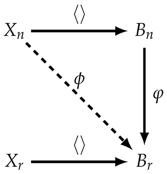
Figure 1. Universal property of a free group $B_n=⟨X_n⟩$.

The group operation, we shall refer to this as a concatenation operation (·), between words $w_1,w_2\in B_n$ is to write $w_1$ and $w_2$ side by side and generate the reduced word in $B_n$. This is denoted by $w=w_1·w_2$ (or $w_1{w}_2$) for any $w_1,w_2\in B_n$. Since the order of $B_n$ is 3, $w·w·w=1$ for all $w\in B_n$. The empty word is the identity in $B_n$ and is represented by 1. Each word in $B_n=⟨X_n⟩$ can also be represented in normal form, as in Equation (4) [8,9]. More comprehensive details are provided in the literature [18,20,22,23,25,27,28].

$$w=\prod _{1\le i\le n}{x}_i^{{\alpha }_i}\prod _{1\le i<j\le n}{[x_i,x_j]}^{{\beta }_{i,j}}\prod _{1\le i<j<k\le n}{[x_i,x_j,x_k]}^{{\gamma }_{i,j,k}}.$$

(4)

In the normal representation of a word w in a Burnside group $B_n$, ${\alpha }_i$, ${\beta }_{i,j}$, ${\gamma }_{i,j,k}$ are the exponents of generators $x_i$, 2-commutators $[x_i,x_j]$, and 3-commutators $[x_i,x_j,x_k]$, respectively. The following example illustrates the transformation of a word in a Burnside group $B_4$.

Example 1.

This is an example of transforming a word $w=x_1^{-1}{x}_2^{-1}{x}_3{x}_1{x}_4$ in a Burnside group $B_4$ with a generating set $X_4=\{x_1,x_2,x_3,x_4\}$ to a corresponding normal representation. Properties associated with commutator words in a Burnside group $B_n$ are discussed in Appendix A. The transformation is as follows, where at each step the bold expression from the previous line is simplified using the underlined transformation in the next line:

$$\begin{array}{cc}\hfill x_1^{-1}{x}_2^{-1}{\mathit{x}}_{\mathbf{3}}{\mathit{x}}_{\mathbf{1}}{x}_4& =x_1^{-1}{x}_2^{-1}\underline{x_1{x}_3{[{\mathit{x}}_{\mathbf{1}},{\mathit{x}}_{\mathbf{3}}]}^{-\mathbf{1}}}{\mathit{x}}_{\mathbf{4}}\hfill \\ \hfill & =x_1^{-1}{\mathit{x}}_{\mathbf{2}}^{-\mathbf{1}}{\mathit{x}}_{\mathbf{1}}{x}_3\underline{x_4{[x_1,x_3]}^{-1}{[x_1,x_3,x_4]}^{-1}}\hfill \\ \hfill & ={\mathit{x}}_{\mathbf{1}}^{-\mathbf{1}}{\mathit{x}}_{\mathbf{1}}{x}_2^{-1}[x_1,x_2]x_3{x}_4{[x_1,x_3]}^{-1}{[x_1,x_3,x_4]}^{-1}\hfill \\ \hfill & =x_2^{-1}[{\mathit{x}}_{\mathbf{1}},{\mathit{x}}_{\mathbf{2}}]{\mathit{x}}_{\mathbf{3}}{x}_4{[x_1,x_3]}^{-1}{[x_1,x_3,x_4]}^{-1}\hfill \\ \hfill & =x_2^{-1}\underline{x_3[x_1,x_2][{\mathit{x}}_{\mathbf{1}},{\mathit{x}}_{\mathbf{2}},{\mathit{x}}_{\mathbf{3}}]}{x}_4{[x_1,x_3]}^{-1}{[x_1,x_3,x_4]}^{-1}\hfill \\ \hfill & =x_2^{-1}{x}_3[{\mathit{x}}_{\mathbf{1}},{\mathit{x}}_{\mathbf{2}}]{\mathit{x}}_{\mathbf{4}}{[x_1,x_3]}^{-1}\underline{[x_1,x_2,x_3]}{[x_1,x_3,x_4]}^{-1}\hfill \\ \hfill & =x_2^{-1}{x}_3\underline{x_4[x_1,x_2][{\mathit{x}}_{\mathbf{1}},{\mathit{x}}_{\mathbf{2}},{\mathit{x}}_{\mathbf{4}}]}{[x_1,x_3]}^{-1}[x_1,x_2,x_3]{[x_1,x_3,x_4]}^{-1}\hfill \\ \hfill & =x_2^{-1}{x}_3{x}_4[x_1,x_2]{[x_1,x_3]}^{-1}[x_1,x_2,x_3]\underline{[x_1,x_2,x_4]}{[x_1,x_3,x_4]}^{-1}\hfill \end{array}$$

The order of a group $B_n$ is $|B_n|=3^{\tilde{n}}$ where $\tilde{n}=n+\left({\displaystyle \genfrac{}{}{0pt}{}{n}{2}}\right)+\left({\displaystyle \genfrac{}{}{0pt}{}{n}{3}}\right)$. The abelianization operation, denoted by $\rho$, is defined in Equation (5), which collects all the generators and corresponding exponents in a word $w\in B_n$ from Equation (4).

$$\rho \left(w\right)=\prod _{1\le i\le n}{x}_i^{{\alpha }_i}$$

(5)

Finitely generated Burnside groups can be geometrically represented using Cayley graphs. The Cayley graph of a Burnside group $B_n$, defined with respect to a generator set $X_n=\{x_1,\dots ,x_n\}$, depicts group words as vertices. Edges connect two vertices if a generator’s (or its inverse) multiplication transforms one into the other. The Cayley distance between two words is the shortest path length between their corresponding vertices in the Cayley graph. The Cayley norm of a word is defined as its distance from the identity word in the Cayley graph. Figure 2 illustrates the partial Cayley graph with essential edges connecting all words in a Burnside group $B_2$ with a generating set $X_2=\{x_1,x_2\}$ in breadth-first order.

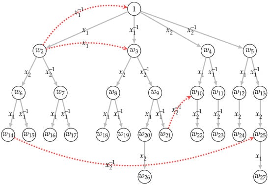
Figure 2. A (partial) Cayley graph of a Burnside group $B_2=⟨X_2⟩$.

2.2. Learning Burnside Homomorphisms with Noise

There exists a homomorphism $\phi :B_n\to B_r$ for any random mapping from a generating set $X_n\subseteq B_n$ to a Burnside group $B_r$. ${\mathsf{\Phi }}_n$ denotes a set of homomorphisms from $B_n$ to $B_r$. For each generator in the generating set $X_n$, there are $|B_r|=3^{\tilde{r}}$ possible mappings where $\tilde{r}=r+\left({\displaystyle \genfrac{}{}{0pt}{}{r}{2}}\right)+\left({\displaystyle \genfrac{}{}{0pt}{}{r}{3}}\right)$. The order of a set of all homomorphisms is $|{\mathsf{\Phi }}_n|=|B_r{|}^n$. The distribution $\mathsf{\Psi }$ represents the error distribution in a set of errors $E\subset B_r$ (Details are illustrated in Section 2.4). For $\phi \in {\mathsf{\Phi }}_n$, the distribution $A_{\phi }^{\mathsf{\Psi }}$ defines the outputs ${\{a_i,w_i\}}_{i=1}^{poly\left(\lambda \right)}$, where $a_i$ is randomly chosen from $B_n$ and $w_i=\phi \left(a_i\right)·e_i$ with $e_i\stackrel{\mathsf{\Psi }}{\leftarrow }E$. On the other hand, the corresponding random distribution $R_{\phi }^{\mathsf{\Psi }}$ defines the outputs ${\{a_i,w_i\}}_{i=1}^{poly\left(\lambda \right)}$, where both $a_i$ and $w_i$ are chosen uniformly from $B_n$ and $B_r$, respectively. Similarly, ${\mathcal{O}}^{A_{\phi }^{\mathsf{\Psi }}}$ and ${\mathcal{O}}^{R_{\phi }^{\mathsf{\Psi }}}$ represent the oracles with distributions $A_{\phi }^{\mathsf{\Psi }}$ and $R_{\phi }^{\mathsf{\Psi }}$, respectively. The decisional $B_n$-LHN problem is to distinguish the oracles ${\mathcal{O}}^{A_{\phi }^{\mathsf{\Psi }}}$ and ${\mathcal{O}}^{R_{\phi }^{\mathsf{\Psi }}}$ with a non-negligible advantage from given polynomial samples. By setting the value of n, a level of security of $nlog\left(\right|B_r\left|\right)$ bits can be achieved from the decisional $B_n$-LHN problem. The security parameter $\lambda$ is defined as $(\tilde{r}log\left(3\right))n$, where $\tilde{r}=r+\left({\displaystyle \genfrac{}{}{0pt}{}{r}{2}}\right)+\left({\displaystyle \genfrac{}{}{0pt}{}{r}{3}}\right)$. Therefore, the decisional $B_n$-LHN assumption is formally stated as follows:

Definition 1 (Decisional B_n-LHN Assumption).

For any $\mathcal{PPT}$ adversary $\mathcal{A}$ and sufficiently large security parameter λ, there exists a negligible function $negl(·)$, such that

$$\left|\underset{\phi \stackrel{\$}{\leftarrow }{\mathsf{\Phi }}_n}{\mathrm{Pr}}\left[{\mathcal{A}}^{{\mathcal{O}}^{A_{\phi }^{\mathsf{\Psi }}}}\left(1^{\lambda }\right)=1\right]-\mathrm{Pr}\left[{\mathcal{A}}^{{\mathcal{O}}^{R_{\phi }^{\mathsf{\Psi }}}}\left(1^{\lambda }\right)=1\right]\right|\le negl\left(\lambda \right).$$

(6)

2.3. Minicrypt Using Burnside Learning Problem

A secret-key cryptosystem utilizes a single secret-key for both encryption and decryption tasks. This shared key is exclusive to the communicating entities and necessitates a secure channel for its distribution. Mathematical functions within symmetric key algorithms facilitate the transformation of plaintext into ciphertext and vice versa. The utilization of a symmetric cryptosystem based on the decisional hardness of the $B_n$-LHN problem is explored in [8]. To encrypt t-bit message m, we define $2^t$ independent words $w_0,w_1,\dots ,w_{2^t-1}$ in $B_r$. Words $w_i$ and $w_j$ are independent if the sets $\{e·w_i:e\in E\}$ and $\{e·w_j:e\in E\}$ are disjoint, for all $0\le i<j\le (2^t-1)$. To encrypt the decimal number m that represents a t-bit message, ciphertext $⟨a,w⟩$ is generated, where $a\stackrel{\$}{\leftarrow }{B}_n$ and $w=\phi \left(a\right)·e·w_m$ for error $e\stackrel{\mathsf{\Psi }}{\leftarrow }E$. A homomorphism $\phi$ sampled uniformly from ${\mathsf{\Phi }}_n$ represents a shared secret-key. To decrypt a ciphertext $⟨a,w⟩$, we compute $w^{\prime }=\phi {\left(a\right)}^{-1}·w$. The plaintext is recovered as m if the word $w^{\prime }$ is in the set $\{e.w_m:e\in E\}$.

2.4. Error Distribution

The security of the $B_n$-LHN learning problem relies on the assumed hardness of group theoretic problems and introduced errors. The introduction of errors contributes to making these problems computationally hard, forming the foundation of the security assumptions. Recall that in the context of the hardness of the $B_n$-LHN problem, we define two Burnside groups $B_n$ and $B_r$ such that $n\gg r\in \mathbb{N}$. The error distribution $\mathsf{\Psi }$ in a Burnside group $B_r$ is generated by concatenating generators from $X_r=\{x_1,\dots ,x_r\}$ in random order, accompanied by random exponents from ternary set $\{0,1,2\}$ [8,9,10].

The probability mass function of errors $e\in B_r$ is precisely defined as follows [8]:

$$\forall e\in B_r,\underset{e\stackrel{\mathsf{\Psi }}{\leftarrow }E}{\mathrm{Pr}}[e\in E]=\underset{\mathbf{v}\stackrel{\$}{\leftarrow }{\mathbb{F}}_3^r,\sigma \stackrel{\$}{\leftarrow }{S}_r}{\mathrm{Pr}}\left[e=\prod x_{{\sigma }_i}^{v_i}\right].$$

(7)

In Equation (7), $v_i$ is the ith component of a vector $\mathbf{v}=(v_1,\dots ,v_r)$ sampled uniformly from a field ${\mathbb{F}}_3^r$. $S_r$ is the set of all permutations of a set $\{1,\dots ,r\}$. The probability mass function in Equation (7) generates a multiset with $r!\times 3^r$ possible errors in $B_r$. The abelianization operation ($\rho$) extracts the generators and their corresponding exponents from a word, while discarding any other exponents, as shown in Equation (5). In a set of samples ${\{a_i,w_i\}}_{i=1}^{poly\left(\lambda \right)}$ with $w_i=\phi \left(a_i\right)·e_i$, $e_i$ represents an error generated according to the distribution $\mathsf{\Psi }$ from a set E. For randomness in abelianized samples ${\{\rho \left(a_i\right),\rho \left(w_i\right)\}}_{i=1}^{poly\left(\lambda \right)}$, an error distribution $\mathsf{\Psi }$ is required. The computation $\rho \left(w_i\right)=\rho \left(\phi \left(a_i\right)\right){+}_3\rho \left(e_i\right)$ ensures randomness, emphasizing the importance of establishing the error distribution $\mathsf{\Psi }$ as defined in Equation (7) to prevent abelianization attacks on the $B_n$-LHN hardness assumption [8].

Let $M=\cup M_l$, $0\le l\le r$ denotes a multiset of errors defined in Equation (7). Here, $M_l$ represents a set of errors with Cayley norm l. Correspondingly, let $E=\bigcup E_l$, where $E_l$ is the associated underlying set of the multiset $M_l$. The function $f:M\to E$ is defined by simplifying an error in M through multiple concatenation operations in the Burnside group $B_r$. The order of the multiset M is $r!\times 3^r$. Similarly, the order of the subsets $M_l$ and $E_l$ is $r!\times 2^l\times \left({\displaystyle \genfrac{}{}{0pt}{}{r}{l}}\right)$ and $l!\times 2^l\times \left({\displaystyle \genfrac{}{}{0pt}{}{r}{l}}\right)$, respectively. Since the function f maps an error from $M_l$ to $E_l$, $M_l$ has precisely $r!/l!$ preimages for an error in $E_l$. In other words, $r!/l!$ errors in $M_l$ constitute different representations for an error in $E_l$. Considering $r!/l!$ identical errors in $M_l$ as a cluster, there are $l!\times 2^l\times \left({\displaystyle \genfrac{}{}{0pt}{}{r}{l}}\right)$ such clusters in $M_l$. The straightforward approach to sample errors according to distribution $\mathsf{\Psi }$ is to determine $\sigma \stackrel{\$}{\leftarrow }{S}_r$, $v\stackrel{\$}{\leftarrow }{\mathbb{F}}_3^r$ as indices and exponents, respectively. However, this approach requires multiple concatenation operations to obtain the simplified error. A bottleneck for cryptosystems based on the $B_n$-LHN assumption arises due to the multiple concatenations for simplifying an error. However, achieving a distribution of errors $\mathsf{\Psi }$ within an error set E can be realized through two distinct methods. In the initial approach, we establish a mapping from a multiset M to an error set E using multiple concatenation operations. This constitutes a one-time precomputation, serving for all subsequent error computations from set E based on the distribution $\mathsf{\Psi }$. As a second approach, we assign the subset $E_l$ an appropriate weight, ensuring that the induced distribution in M is uniform, a requirement for the $B_n$-LHN cryptosystem. By assigning a distribution weight to the subset $E_l$ as $(2^l\times \left({\displaystyle \genfrac{}{}{0pt}{}{r}{l}}\right))/3^r$, we can achieve a uniform distribution of M, representing the distribution $\mathsf{\Psi }$ of E [10].

3. Bn Optimization

The cryptographic primitives developed in this study are constructed based on the $B_n$-LHN hardness assumption. The $B_n$-LHN hardness assumption assures that no $\mathcal{PPT}$ adversary distinguishes the outputs ${\{a_i,w_i\}}_{i=1}^{poly\left(\lambda \right)}$ from random outputs with non-negligible advantage, see Definition (1). Here, $w_i=\phi \left(a_i\right)·e_i$ and $\phi$ is a secret-homomorphism sampled uniformly from ${\mathsf{\Phi }}_n$. The error $e_i$ is sampled from a set of errors E according to the distribution $\mathsf{\Psi }$ and (·) is the concatenation operation. Cryptographic primitives leveraging the $B_n$-LHN problem require an optimized design for two key operations: 1. Concatenation operations within the Burnside groups $B_n$ and $B_r$. 2. Homomorphisms from a Burnside group $B_n$ to a Burnside group $B_r$ for $n\gg r\in \mathbb{N}$. In this section, an efficient concatenation operation is introduced within the Burnside groups $B_n$ and $B_r$ for $n\gg r\in \mathbb{N}$, highlighting a parallel approach.

3.1. Representation of a Word

The most fundamental operation within the Burnside groups is the concatenation operation. To achieve an efficient concatenation operation, we utilize the standard representation of a word w in a Burnside group $B_n$, as displayed in Equation (4). The normal representation of a word w in $B_n$ comprises approximately $O\left(n\right)$ generators, $O\left(n^2\right)$ 2-commutators, and $O\left(n^3\right)$ 3-commutators alongside their respective exponents. To execute the concatenation operation, it suffices to store the exponents of generators, 2-commutators, and 3-commutators of a word w as a sequence. Figure 3 shows a word w in a Burnside group $B_n$. In memory, a word w in a Burnside group $B_n$ requires the space for n exponents for generators, $\left({\displaystyle \genfrac{}{}{0pt}{}{n}{2}}\right)$ exponents for 2-commutators, and $\left({\displaystyle \genfrac{}{}{0pt}{}{n}{3}}\right)$ exponents for 3-commutators.

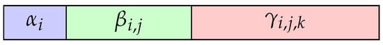
Figure 3. Normal representation of a word $w\in B_n$.

The first block of a word w in Figure 3 sequentially holds the exponents ${\alpha }_i$ for $1\le i\le n$. We shall refer to this as the alpha-block of a word w for future convenience. The second block of a word w, referred to as the beta-block, sequentially stores the exponents ${\beta }_{i,j}$ for $1\le i<j\le n$. The beta-block contains $\left({\displaystyle \genfrac{}{}{0pt}{}{n}{2}}\right)$ exponents. The third block of a word w, known as the gamma-block, sequentially contains the exponents ${\gamma }_{i,j,k}$ for $1\le i<j<k\le n$. The gamma-block encompasses $\left({\displaystyle \genfrac{}{}{0pt}{}{n}{3}}\right)$ exponents. Collectively, we represent a word $w\in B_n$ as $w=\{{\alpha }_i,{\beta }_{i,j},{\gamma }_{i,j,k}\}$ for $1\le i<j<k\le n$.

3.2. Computing the Group Operation: The Collecting Process

To concatenate words $w_1$ and $w_2$ in a Burnside group $B_n$, represented as $w=w_1·w_2$, we utilize a three-stage collecting process. For $1\le i<j<k\le n$, let ${\alpha }_i$, ${\beta }_{i,j}$, and ${\gamma }_{i,j,k}$ be the corresponding exponents in the alpha-block, beta-block, and gamma-block in the resultant word $w=\{{\alpha }_i,{\beta }_{i,j},{\gamma }_{i,j,k}\}=w_1·w_2\in B_n$, respectively. Furthermore, let the words $w_1$ and $w_2$ be defined as $\{{\alpha }_i^{\left(1\right)},{\beta }_{i,j}^{\left(1\right)},{\gamma }_{i,j,k}^{\left(1\right)}\}$ and $\{{\alpha }_i^{\left(2\right)},{\beta }_{i,j}^{\left(2\right)},{\gamma }_{i,j,k}^{\left(2\right)}\}$, respectively.

In stage 1 of the collecting process, the exponent ${\gamma }_{i,j,k}^{\left(1\right)}$ in the gamma-block of $w_1$ merges with the corresponding exponent ${\gamma }_{i,j,k}^{\left(2\right)}$ in the gamma-block of $w_2$, as shown in Figure 4. Since the 3-commutator commutes with everything, as in Property (4), the time complexity to merge an exponent ${\gamma }_{i,j,k}^{\left(1\right)}$ with the corresponding exponent ${\gamma }_{i,j,k}^{\left(2\right)}$ is $O\left(1\right)$. Since there are $O\left(n^3\right)$ exponents in the gamma-block of $w_1$, the time complexity to merge the gamma-block of $w_1$ with the gamma-block of $w_2$ is $O\left(n^3\right)$.

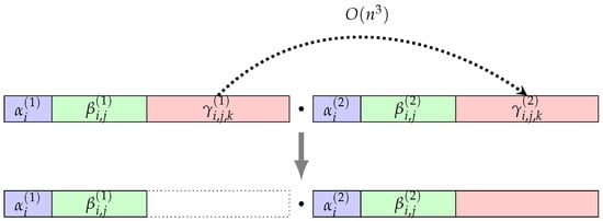
Figure 4. Collecting process (stage 1).

In stage 2, the exponent ${\beta }_{i,j}^{\left(1\right)}$ in the beta-block of $w_1$ merges with the corresponding exponent ${\beta }_{i,j}^{\left(2\right)}$ in the beta-block of $w_2$, as shown in Figure 5. During the merge, the exponent ${\beta }_{i,j}^{\left(1\right)}$ swaps with the exponents ${\alpha }_k^{\left(2\right)}$ in the alpha block of $w_2$. Each swap between ${\beta }_{i,j}^{\left(1\right)}$ and ${\alpha }_k^{\left(2\right)}$ generates a 3-commutator exponent, as in Property (2), which can freely move towards the gamma-block of the resulting word w with $O\left(1\right)$ complexity. Since there are $O\left(n^2\right)$ exponents in the beta-block of $w_1$ that swap with the $O\left(n\right)$ exponents in the alpha-block of $w_2$, the time complexity for stage 2 is $O\left(n^3\right)$.

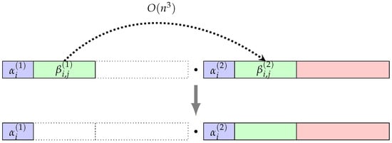
Figure 5. Collecting process (stage 2).

In the final stage, the lexicographical order among exponents in the alpha-block of $w_1$ and alpha-block of $w_2$ is restored, as shown in Figure 6. The swapping among the exponents of the alpha-blocks of $w_1$ and $w_2$ creates a 2-commutator exponent, as in Property (1). The generated 2-commutator exponent crosses the exponents in the remaining alpha-block of $w_2$ to merge into the beta-block of the resultant word w. Since there are $O\left(n^2\right)$ swaps among generators in the alpha-blocks of $w_1$ and $w_2$, and as there are at most $O\left(n\right)$ crossings for each generated 2-commutator exponent, the time complexity for stage 3 is $O\left(n^3\right)$.

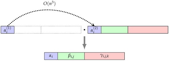
Figure 6. Collecting process (stage 3).

Example 2 illustrates the collecting process of a concatenation operation in a Burnside group $B_4$.

Example 2.

In a Burnside group $B_4$ with a generating set $X_4=\{x_1,x_2,x_3,x_4\}$, let $w_1=x_1{x}_2^{-1}{x}_3[x_2,x_3]{[x_1,x_2,x_3]}^{-1}$ and $w_2=x_2{x}_3^{-1}[x_1,x_2]{[x_1,x_3]}^{-1}[x_2,x_3]$ be two words in $B_n$. The concatenation operation using the three-stage collecting process in $w=w_1·w_2$ is computed as follows, where at each step the bold expression from the previous line is simplified using the underlined transformation in the next line:

$$\begin{array}{cc}\hfill w& =w_1·w_2\hfill \\ \hfill & =x_1{x}_2^{-1}{x}_3[x_2,x_3]{[{\mathit{x}}_{\mathbf{1}},{\mathit{x}}_{\mathbf{2}},{\mathit{x}}_{\mathbf{3}}]}^{-\mathbf{1}}·x_2{x}_3^{-1}[x_1,x_2]{[x_1,x_3]}^{-1}[x_2,x_3]\hfill \\ \hfill & =x_1{x}_2^{-1}{x}_3[{\mathit{x}}_{\mathbf{2}},{\mathit{x}}_{\mathbf{3}}]{\mathit{x}}_{\mathbf{2}}{x}_3^{-1}[x_1,x_2]{[x_1,x_3]}^{-1}[x_2,x_3]\underline{{[x_1,x_2,x_3]}^{-1}}\hfill \\ \hfill & =x_1{x}_2^{-1}{x}_3\underline{x_2[{\mathit{x}}_{\mathbf{2}},{\mathit{x}}_{\mathbf{3}}]}{\mathit{x}}_{\mathbf{3}}^{-\mathbf{1}}[x_1,x_2]{[x_1,x_3]}^{-1}[x_2,x_3]{[x_1,x_2,x_3]}^{-1}\hfill \\ \hfill & =x_1{x}_2^{-1}{\mathit{x}}_{\mathbf{3}}{\mathit{x}}_{\mathbf{2}}\underline{x_3^{-1}[{\mathit{x}}_{\mathbf{2}},{\mathit{x}}_{\mathbf{3}}]}[x_1,x_2]{[x_1,x_3]}^{-1}[{\mathit{x}}_{\mathbf{2}},{\mathit{x}}_{\mathbf{3}}]{[x_1,x_2,x_3]}^{-1}\hfill \\ \hfill & =x_1{\mathit{x}}_{\mathbf{2}}^{-\mathbf{1}}\underline{{\mathit{x}}_{\mathbf{2}}{\mathit{x}}_{\mathbf{3}}{[{\mathit{x}}_{\mathbf{2}},{\mathit{x}}_{\mathbf{3}}]}^{-\mathbf{1}}}{\mathit{x}}_{\mathbf{3}}^{-\mathbf{1}}[x_1,x_2]{[x_1,x_3]}^{-1}\underline{{[x_2,x_3]}^{-1}}{[x_1,x_2,x_3]}^{-1}\hfill \\ \hfill & =x_1\underline{{\mathit{x}}_{\mathbf{3}}{\mathit{x}}_{\mathbf{3}}^{-\mathbf{1}}{[{\mathit{x}}_{\mathbf{2}},{\mathit{x}}_{\mathbf{3}}]}^{-\mathbf{1}}}[x_1,x_2]{[x_1,x_3]}^{-1}{[{\mathit{x}}_{\mathbf{2}},{\mathit{x}}_{\mathbf{3}}]}^{-\mathbf{1}}{[x_1,x_2,x_3]}^{-1}\hfill \\ \hfill & =x_1[x_1,x_2]{[x_1,x_3]}^{-1}\underline{[x_2,x_3]}{[x_1,x_2,x_3]}^{-1}\hfill \end{array}$$

3.3. Computing the Group Operation: A Direct Approach

For the subsequent discussions, we use the following properties associated with exponents of generators, 2-commutators, and 3-commutators. The properties follow from the details as discussed in Appendix A.

Property 1 (Swapping Generators).

Let $w_1$ and $w_2$ be words in a Burnside group $B_n$, defined as $\{{\alpha }_i^{\left(1\right)},{\beta }_{i,j}^{\left(1\right)},{\gamma }_{i,j,k}^{\left(1\right)}\}$ and $\{{\alpha }_i^{\left(2\right)},{\beta }_{i,j}^{\left(2\right)},{\gamma }_{i,j,k}^{\left(2\right)}\}$, respectively. For $1\le i<j<k\le n$, the collecting process in $w=\{{\alpha }_i,{\beta }_{i,j},{\gamma }_{i,j,k}\}=w_1·w_2$ allows the swapping of exponents ${\alpha }_j^{\left(1\right)}$ and ${\alpha }_i^{\left(2\right)}$, updating the resulting exponent ${\beta }_{i,j}$ as follows: ${\beta }_{i,j}={\beta }_{i,j}{+}_3{\alpha }_j^{\left(1\right)}{\times }_3{\alpha }_i^{\left(2\right)}{\times }_{3}2$.

Property 2 (Swapping 2-Commutator and Generator).

Let $w_1$ and $w_2$ be words in a Burnside group $B_n$, defined as $\{{\alpha }_i^{\left(1\right)},{\beta }_{i,j}^{\left(1\right)},{\gamma }_{i,j,k}^{\left(1\right)}\}$ and $\{{\alpha }_i^{\left(2\right)},{\beta }_{i,j}^{\left(2\right)},{\gamma }_{i,j,k}^{\left(2\right)}\}$, respectively. For $1\le i<j\le n$ and $1\le k\le n$ with $k\ne i$ and $k\ne j$, the collecting process in $w=\{{\alpha }_i,{\beta }_{i,j},{\gamma }_{i,j,k}\}=w_1·w_2$ allows the swapping of exponents ${\beta }_{i,j}^{\left(1\right)}$ and ${\alpha }_k^{\left(2\right)}$. The swap updates the resultant exponent ${\gamma }_{i,j,k}$ in two scenarios:  

Case I: 

If $j<k$ or $k<i$, ${\gamma }_{i,j,k}={\gamma }_{i,j,k}{+}_3{\beta }_{i,j}^{\left(1\right)}{\times }_3{\alpha }_k^{\left(2\right)}$.

Case I: 

If $i<k<j$, ${\gamma }_{i,j,k}={\gamma }_{i,j,k}{+}_3{\beta }_{i,j}^{\left(1\right)}{\times }_3{\alpha }_k^{\left(2\right)}{\times }_{3}2$.

Note: If $k=i$ or $k=j$, the collecting process in $w=w_1·w_2$ allows the swapping of exponents ${\beta }_{i,j}^{\left(1\right)}$ and ${\alpha }_k^{\left(2\right)}$ without necessitating updates to the resultant exponent ${\gamma }_{i,j,k}$.

Property 3 (Swapping 2-Commutators).

Let $w_1$ and $w_2$ be words in a Burnside group $B_n$, defined as $\{{\alpha }_i^{\left(1\right)},{\beta }_{i,j}^{\left(1\right)},{\gamma }_{i,j,k}^{\left(1\right)}\}$ and $\{{\alpha }_i^{\left(2\right)},{\beta }_{i,j}^{\left(2\right)},{\gamma }_{i,j,k}^{\left(2\right)}\}$, respectively. For $1\le i<j\le n$ and $1\le s<t\le n$, the collecting process in $w=w_1·w_2$ allows the swapping of exponents ${\beta }_{i,j}^{\left(1\right)}$ and ${\beta }_{s,t}^{\left(2\right)}$ without requiring updates to the resultant exponents.

Property 4 (Swapping 3-Commutator with Everything).

Let the words $w_1$ and $w_2$ in a Burnside group $B_n$ be defined as $\{{\alpha }_i^{\left(1\right)},{\beta }_{i,j}^{\left(1\right)},{\gamma }_{i,j,k}^{\left(1\right)}\}$ and $\{{\alpha }_i^{\left(2\right)},{\beta }_{i,j}^{\left(2\right)},{\gamma }_{i,j,k}^{\left(2\right)}\}$, respectively. For $1\le i<j<k\le n$ and $1\le s\le n$, the collecting process in $w=w_1·w_2$ allows the swapping of exponents ${\gamma }_{i,j,k}^{\left(1\right)}$ and ${\alpha }_s^{\left(2\right)}$ without requiring updates to the resultant exponents. Similarly, for $1\le i<j<k\le n$ and $1\le s<t\le n$, the collecting process in $w=w_1·w_2$ allows the swapping between exponents ${\gamma }_{i,j,k}^{\left(1\right)}$ and ${\beta }_{s,t}^{\left(2\right)}$ without requiring updates to the resultant exponents. Likewise, for $1\le i<j<k\le n$ and $1\le s<t<u\le n$, the collecting process in $w=w_1·w_2$ allows the swapping between exponents ${\gamma }_{i,j,k}^{\left(1\right)}$ and ${\gamma }_{s,t,u}^{\left(2\right)}$ without requiring updates to the resultant exponents.

Utilizing the idea of the collecting process, we design a direct concatenation operation to generate the resultant word $w=w_1·w_2$ for $1\le i<j<k\le n$, as shown in Algorithm 1. Note: ${+}_3$ and ${\times }_3$ are addition and multiplication mod 3 operations, respectively.    

Algorithm 1: Direct concatenation operation (·)

3.4. Computing the Group Operation: A Parallelizable Direct Approach

The direct concatenation operation defined for a Burnside group $B_n$ that utilizes the collecting process requires $O\left(n^3\right)$ time complexity, as illustrated in Algorithm 1. In this section, we enhance the design of the direct concatenation operation in Algorithm 1, where we can utilize parallel computation. We shall refer to this as a parallelizable direct concatenation operation. To achieve a parallelizable direct concatenation operation, we further extend the memory representation of the alpha-block, beta-block, and gamma-block of a word in a Burnside group $B_n$. We employ the Type I and Type II representations proposed by [29].

3.5. Parallel Addition and Multiplication mod 3

For the subsequent discussion, we introduce a parallel design for member-wise addition modulo 3 and multiplication modulo 3, crucial for implementing the parallelizable concatenation operation. To illustrate, let us examine the initial computation ${\alpha }_i\leftarrow {\alpha }_i^{\left(1\right)}{+}_3{\alpha }_i^{\left(2\right)}$ from Algorithm 1. With the naive approach, we can formulate the $O\left(n\right)$ algorithm, as depicted in Algorithm 2.    

Algorithm 2: $O\left(n\right)$ addition modulo 3 operation

For the parallel design of the addition modulo 3 and multiplication modulo 3, we employ two binary arrays of size n, namely $\alpha msb$ and $\alpha lsb$, in lieu of a ternary array $\alpha$ of the same size. This is denoted as $\alpha \stackrel{·}{=}\{\alpha msb,\alpha lsb\}$. The transformation from the ternary array $\alpha$ to its equivalent binary representations $\alpha msb$ and $\alpha lsb$ is conducted as follows: If ${\alpha }_i$ is 0, both corresponding bits $\alpha {msb}_i$ and $\alpha {lsb}_i$ are set to 0. In the case where ${\alpha }_i$ is 1, the $\alpha {msb}_i$ bit is set to 0, and the $\alpha {lsb}_i$ bit is set to 1. Finally, if ${\alpha }_i$ is 2, the $\alpha {msb}_i$ bit is set to 1, and the $\alpha {lsb}_i$ bit is set to 0. Similarly, the binary representations for an alpha-block ($\alpha$), beta-block ($\beta$), and gamma-block ($\gamma$) for a word w are shown in Figure 7.

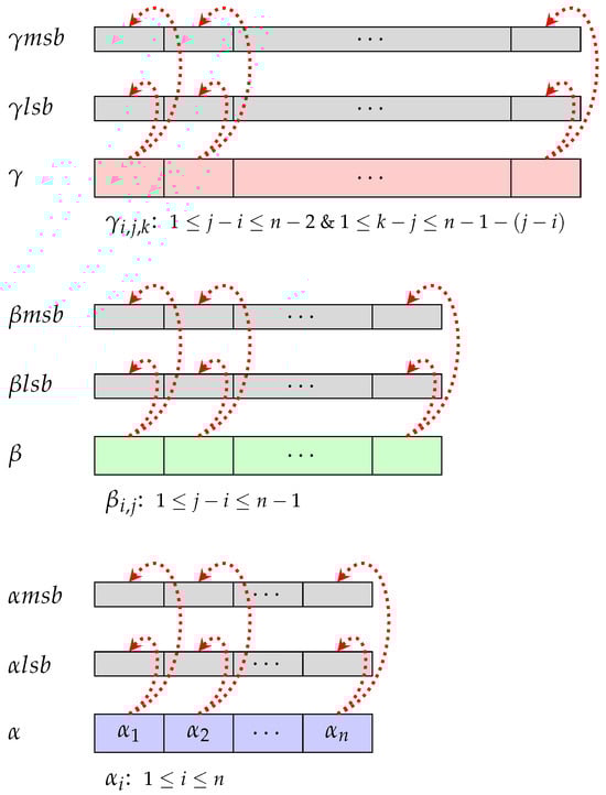
Figure 7. Memory representation of a word in $B_n$.

Utilizing Algorithm 3, we achieve $O\left(1\right)$ time complexity in a parallel setting, a significant improvement compared to Algorithm 2, for the computation ${\alpha }_i\leftarrow {\alpha }_i^{\left(1\right)}{+}_3{\alpha }_i^{\left(2\right)}$ for $1\le i\le n$. This computation can be implemented with just seven machine instructions. Similarly, we achieve the $O\left(1\right)$ time complexity in a parallel setting for ${\alpha }_i\leftarrow {\alpha }_i^{\left(1\right)}{\times }_3{\alpha }_i^{\left(2\right)}$ for $1\le i\le n$ using Algorithm 4. This provides a streamlined and efficient approach for both addition and multiplication operations in comparison to the previously mentioned Algorithm 2. From now on, we represent the parallel designs for ${\alpha }_i\leftarrow {\alpha }_i^{\left(1\right)}{+}_3{\alpha }_i^{\left(2\right)}$ and ${\alpha }_i\leftarrow {\alpha }_i^{\left(1\right)}{\times }_3{\alpha }_i^{\left(2\right)}$ for $1\le i\le n$ as $\alpha \leftarrow {\alpha }^{\left(1\right)}{\times }_3{\alpha }^{\left(2\right)}$ and $\alpha \leftarrow {\alpha }^{\left(1\right)}{\odot }_3{\alpha }^{\left(2\right)}$, respectively, without using the indices. This simplification enhances the clarity and conciseness in our notation. Equivalent parallel designs are depicted in Figure 8 and Figure 9.

Algorithm 3: Parallel addition mod 3 operation, ${+}_3$

Data: Ternary arrays ${\alpha }^{\left(1\right)}\stackrel{·}{=}\{{\alpha }^{\left(1\right)}msb,{\alpha }^{\left(1\right)}lsb\}$ and ${\alpha }^{\left(2\right)}\stackrel{·}{=}\{{\alpha }^{\left(2\right)}msb,{\alpha }^{\left(2\right)}lsb\}$ of size n Result: Ternary array $\alpha \stackrel{·}{=}\{\alpha msb,\alpha lsb\}$ of size n for the member-wise addition mod 3, where $\alpha \leftarrow {\alpha }^{\left(1\right)}{+}_3{\alpha }^{\left(2\right)}$ $t\leftarrow ({\alpha }^{\left(1\right)}msb\mid {\alpha }^{\left(2\right)}lsb)\oplus ({\alpha }^{\left(1\right)}lsb\mid {\alpha }^{\left(2\right)}msb))$ $\alpha msb\leftarrow (({\alpha }^{\left(1\right)}lsb\mid {\alpha }^{\left(2\right)}lsb)\oplus t)$ $\alpha lsb\leftarrow (({\alpha }^{\left(1\right)}msb\mid {\alpha }^{\left(2\right)}msb)\oplus t)$

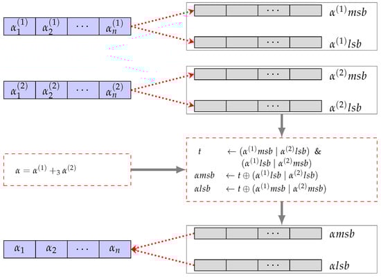
Figure 8. Parallel addition mod 3 operation.

Figure 9. Parallel multiplication mod 3 operation.

Algorithm 4: Parallel multiplication mod 3 operation, ${\odot }_3$

Data: Ternary arrays ${\alpha }^{\left(1\right)}\stackrel{·}{=}\{{\alpha }^{\left(1\right)}msb,{\alpha }^{\left(1\right)}lsb\}$ and ${\alpha }^{\left(2\right)}\stackrel{·}{=}\{{\alpha }^{\left(2\right)}msb,{\alpha }^{\left(2\right)}lsb\}$ of size n Result: Ternary array $\alpha \stackrel{·}{=}\{\alpha msb,\alpha lsb\}$ of size n for the member-wise multiplication mod 3, where $\alpha \leftarrow {\alpha }^{\left(1\right)}{\odot }_3{\alpha }^{\left(2\right)}$ $\alpha msb\leftarrow (\overline{{\alpha }^{\left(1\right)}msb}\&{\alpha }^{\left(1\right)}lsb\&\overline{{\alpha }^{\left(2\right)}msb}\&{\alpha }^{\left(2\right)}lsb)\mid ({\alpha }^{\left(1\right)}msb\&\overline{{\alpha }^{\left(1\right)}lsb}\&{\alpha }^{\left(2\right)}msb\&\overline{{\alpha }^{\left(2\right)}lsb})$ $\alpha lsb\leftarrow (\overline{{\alpha }^{\left(1\right)}msb}\&{\alpha }^{\left(1\right)}lsb\&{\alpha }^{\left(2\right)}msb\&\overline{{\alpha }^{\left(2\right)}lsb})\mid ({\alpha }^{\left(1\right)}msb\&\overline{{\alpha }^{\left(1\right)}lsb}\&\overline{{\alpha }^{\left(2\right)}msb}\&{\alpha }^{\left(2\right)}lsb)$

3.6. Multi-Block Representation of a Word

The extended memory representation of a word $w=\{{\alpha }_i,{\beta }_{i,j},{\gamma }_{i,j,k}\}$ in a Burnside group $B_n$ to achieve $O\left(n^2\right)$ time complexity is visualized as follows: Note: One block is an n-sized array filled from left to right in chronological order.

3.6.1. Representation of Alpha-Block

To represent an alpha-block of a word $w=\{{\alpha }_i,{\beta }_{i,j},{\gamma }_{i,j,k}\}$, we define a block $\alpha$ that stores all exponents ${\alpha }_i$ for $1\le i\le n$. That is, the block $\alpha$ stores the entries $\{{\alpha }_1,\dots ,{\alpha }_n\}$.

3.6.2. Representation of Beta-Block

To represent a beta-block of a word $w=\{{\alpha }_i,{\beta }_{i,j},{\gamma }_{i,j,k}\}$, we define n-sized blocks $\beta \left\{l\right\}$ for $1\le l\le (n-1)$. The block $\beta \left\{l\right\}$ stores all exponents ${\beta }_{i,j}$, such that $j=i+l$ for $1\le i<j\le n$ from left to right. The remaining entries are set to zero. For instance, the block $\beta \left\{1\right\}$ stores the exponents $\{{\beta }_{1,2},{\beta }_{2,3},{\beta }_{3,4},\dots ,{\beta }_{n-2,n-1},{\beta }_{n-1,n},0\}$. The last entry in the block $\beta \left\{1\right\}$ is set to zero. Similarly, the last block $\beta \{n-1\}$ stores only exponent ${\beta }_{1,n}$ as $\{{\beta }_{1,n},0,0,\dots ,0,0,0\}$. All other entries except the first in the block $\beta \{n-1\}$ are set to zero.

3.6.3. Representation of Gamma-Block

To represent a gamma-block of a word $w=\{{\alpha }_i,{\beta }_{i,j},{\gamma }_{i,j,k}\}$, we define n-sized blocks $\gamma \left\{l_1\right\}\left\{l_2\right\}$ for $1\le l_1\le (n-2)$ and $1\le l_2\le (n-1)-l_1$. The block $\gamma \left\{l_1\right\}\left\{l_2\right\}$ stores all exponents ${\gamma }_{i,j,k}$, such that $j=i+l_1$ and $k=j+l_2$ for $1\le i<j<k\le n$ from left to right in a chronological order. The remaining entries are set to zero. For instance, the block $\gamma \left\{1\right\}\left\{1\right\}$ stores the exponents $\{{\gamma }_{1,2,3},{\beta }_{2,3,4},{\gamma }_{3,4,5},\dots ,{\gamma }_{n-2,n-1,n},0,0\}$. The last two entries in the block $\gamma \left\{1\right\}\left\{1\right\}$ are set to zero. Similarly, the last block $\gamma \{n-2\}\left\{1\right\}$ stores only exponent ${\gamma }_{1,n-1,n}$ as $\{{\gamma }_{1,n-1,n},0,0,\dots ,0,0,0\}$. All other entries except the first in the block $\gamma \{n-2\}\left\{1\right\}$ are set to zero.

Utilizing the multi-block structure, we can represent a word $w=\{{\alpha }_i,{\beta }_{i,j},{\gamma }_{i,j,k}\}$ in a Burnside group $B_n$ as $w=\{\alpha ,\beta \left\{l_1\right\},\gamma \left\{l_2\right\}\left\{l_3\right\}\}$, where $1\le l_1\le (n-1)$, $1\le l_2\le (n-2)$, and $1\le l_3\le ((n-1)-l_2)$. Similarly, we represent words $w_1=\{{\alpha }_i^{\left(1\right)},{\beta }_{i,j}^{\left(1\right)},{\gamma }_{i,j,k}^{\left(1\right)}\}$ and $w_2=\{{\alpha }_i^{\left(2\right)},{\beta }_{i,j}^{\left(2\right)},{\gamma }_{i,j,k}^{\left(2\right)}\}$ in a multi-block structure as $w_1=\{{\alpha }^{\left(1\right)},{\beta }^{\left(1\right)}\left\{l_1\right\},{\gamma }^{\left(1\right)}\left\{l_2\right\}\left\{l_3\right\}\}$ and $w_2=\{{\alpha }^{\left(2\right)},{\beta }^{\left(2\right)}\left\{l_1\right\},{\gamma }^{\left(2\right)}\left\{l_2\right\}\left\{l_3\right\}\}$ for $1\le l_1\le (n-1)$, $1\le l_2\le (n-2)$, and $1\le l_3\le ((n-1)-l_2)$. Algorithm 5 demonstrates the parallelizable direct concatenation operation in a Burnside group $B_n$ using the parallel block-addition and block-multiplication from Algorithm 3 and Algorithm 4, respectively.

Algorithm 5: Parallelizable direct concatenation operation (·)

3.7. Homomorphism Optimization

A homomorphism from a Burnside group $B_n=⟨X_n⟩$, where $X_n=\{x_1,\dots ,x_n\}$, to another Burnside group $B_r$ is defined as a mapping from a generator $x_i$ to a word $w_i\in B_r$. Consequently, a homomorphism $\phi \in {\mathsf{\Phi }}_n$ is represented as $\phi =\{w_1,\dots ,w_n\}$, where $w_i\in B_r$. Consider a word $a=\{{\alpha }_i,{\beta }_{i,j},{\gamma }_{i,j,k}\}$ in a Burnside group $B_n$ with exponents ${\alpha }_i$, ${\beta }_{i,j}$, and ${\gamma }_{i,j,k}$ in the alpha-block, beta-block, and gamma-block, respectively, for $1\le i<j<k\le n$. The computation of the homomorphism in a word $a\in B_n$, denoted as $\phi \left(a\right)$, is as Equation (8).

$$\phi \left(a\right)=\prod _{1\le i\le n}{w}_i^{{\alpha }_i}\prod _{1\le i<j\le n}{[w_i,w_j]}^{{\beta }_{i,j}}\prod _{1\le i<j<k\le n}{[w_i,w_j,w_k]}^{{\gamma }_{i,j,k}}.$$

(8)

As a naive approach, a 2-commutator $[w_i,w_j]=w_i^{-1}·w_j^{-1}·w_i·w_j$ and a 3-commutator $[w_i,w_j,w_k]={[w_i,w_j]}^{-1}·w_k^{-1}·[w_i,w_j]·w_k$ requires 3 and 9 concatenation operations in $B_r$, respectively. Note: We calculate the inverse of a word $w\stackrel{·}{=}\{wmsb,wlsb\}$ as $w^{-1}\stackrel{·}{=}\{wlsb,wmsb\}$. However, while performing the homomorphism, there are many duplicate computations. For example, we can reuse the 2-commutator $[w_i,w_j]$ in the computation $[w_i,w_j,w_k]$. Thus, to optimize the homomorphism computation, we generate weight-2 and weight-3 look-up tables that store 2-commutators ($[w_i,w_j]$) and 3-commutators ($[w_i,w_j,w_k]$), respectively. For a given homomorphism $\phi \in {\mathsf{\Phi }}_n$, generating weight-2 and weight-3 look-up tables is a one-time precomputation and can be utilized for all subsequent computations in $\phi \left(a\right)$.

4. PRF Construction

In this section, we design three progressively refined constructions of a PRF family using the GGM approach, grounded in the $B_n$-LHN assumption. The primary challenge in designing a PRF based on the $B_n$-LHN assumption lies in managing the errors associated with it. The key idea here, in the PRF designs, is to extract errors from the secret-key of the underlying PRF. The initial PRG design, termed the direct PRG, applies the $B_n$-LHN assumption by capitalizing on the lower entropy of a set of errors E compared to a Burnside group $B_r$. In the second approach, we introduce a PRG design, referred to as the parameterized PRG, where the function description of a PRG is derived from the public parameters and secret-key of the underlying PRF. Although this may seem counterintuitive at first, our findings indicate that the intermediate PRG used in the GGM’s PRG-based PRF construction places a less strict requirement on the PRG itself, as discussed in the following outlines. In the final approach, we propose a design called an indexed PRG with a set of public parameters and an index associated with it.

Construction 1 (Direct PRG). 

Let $\phi$ be a homomorphism in ${\mathsf{\Phi }}_n$. For some $t,l,l^{\prime }\in \mathbb{N}$, we define a function $G:{\{0,1\}}^l\to {\{0,1\}}^{l^{\prime }}$ with $l^{\prime }>l$ as follows:

$$G(\phi ,a_1,e_1,\dots ,a_t,e_t)=⟨a_1,w_1,\dots ,a_t,w_t⟩,$$

(9)

where each $w_i$ is computed as $w_i=\phi \left(a_i\right)·e_i$ for $1\le i\le t$. Here, the values $a_i$ are sampled from the Burnside group $B_n$, while $e_i$ are chosen from the error set E.

The input and output bit sizes of G are given by $l=\overline{w}n+t(p+\overline{e})$ and $l^{\prime }=t(p+\overline{w})$, respectively. Here, p and $\overline{w}$ denote the entropy of the Burnside groups $B_n$ and $B_r$, respectively, while $q=\overline{w}n$ represents the entropy of the homomorphism set ${\mathsf{\Phi }}_n$, and $\overline{e}$ characterizes the entropy of the error set $E\subset B_r$.

Theorem 1.

If the $B_n$-LHN assumption holds and $t>{\displaystyle \frac{\overline{w}n}{\overline{w}-\overline{e}}}$, then the function G from Construction 1 is a PRG.

Proof. 

The proof follows directly from the $B_n$-LHN assumption. A function G qualifies as a PRG if its output bit length exceeds its input bit length.

The input bit size of G is given by $l=\overline{w}n+t(p+\overline{e})$, while the output bit size is $l^{\prime }=t(p+\overline{w})$. For G to be a PRG, it must satisfy $l^{\prime }>l$, which simplifies to

$$t(p+\overline{w})>\overline{w}n+t(p+\overline{e}).$$

Rearranging the inequality, we obtain

$$t(\overline{w}-\overline{e})>\overline{w}n.$$

Solving for t, we obtain the required bound:

$$t>{\displaystyle \frac{\overline{w}n}{\overline{w}-\overline{e}}}.$$

Since the entropy of the set of errors E (denoted by $\overline{e}$) is smaller than the entropy of the Burnside group $B_r$ (denoted by $\overline{w}$), we can select a sufficiently large t to overcome the entropy $q=\overline{w}n$ in the input of G. This ensures that the entropy of the output of G exceeds that of its input, thereby establishing G as a PRG. □

Construction 2 (PRF from Direct PRG).

(Outline) We construct a PRF by utilizing a length-stretching PRG G from Construction 1 as follows: First, we construct a length-doubling PRG $\tilde{G}$ from a length-stretching PRG G by cascading multiple PRGs in series. Second, we define a PRF $f_k$, for any input $x=x_1\dots x_m$ and secret-key k, using the GGM approach as follows:

$$f_k(x_1\dots x_m)={\tilde{G}}^{\left(x_m\right)}(\dots \left({\tilde{G}}^{\left(x_2\right)}\left({\tilde{G}}^{\left(x_1\right)}\left(k\right)\right)\right)\dots ).$$

The secret-key k is $\{\phi ,a_1,e_1,\dots ,a_t,e_t\}$ where $\phi$ is sampled from a set of homomorphisms ${\mathsf{\Phi }}_n$. Moreover, $a_i\in B_n$, $e_i\in E$ for $1\le i\le t$. The size of the secret-key k is $\overline{w}n+t(p+\overline{e})$ where $t={\displaystyle \frac{\overline{w}n+1}{\overline{w}-\overline{e}}}$. However, a disadvantage of this construction appears to be a notably large secret-key size, even for small values of n.

We suggest an adjustment to the direct PRG, leading to a significant decrease in the secret-key size of a PRF. This reduction is considerable, particularly for a large enough n, reducing the key size significantly. This modified construction introduces extra public parameters and is denoted as the parameterized PRG. The construction is detailed as follows:

Construction 3 (Parameterized PRG).

Let $\phi$ be a homomorphism in ${\mathsf{\Phi }}_n$. For some $t,l,l^{\prime }\in \mathbb{N}$, a function $G:{\{0,1\}}^l\to {\{0,1\}}^{l^{\prime }}$ with $l^{\prime }>l$ is defined as

$$G(\phi ,e_1,\dots ,e_t)=⟨w_1,\dots ,w_t⟩$$

(10)

For $1\le i\le t$, $w_i=\phi \left(a_i\right)·e_i$ and $e_i\in E$. Furthermore, $a_i\in B_n$ is a public parameter associated with an error $e_i$. Here, the input and output bit size of a function G are $l=\overline{w}n+t\overline{e}$ and $l^{\prime }=\overline{w}t$, respectively.

Claim 1.

Length-doubling parameterized PRG is sufficient for a GGM PRG-based PRF approach, as demonstrated in Construction 3 and Theorem 2.

Theorem 2.

Let the $B_n$-LHN assumption hold and $t>{\displaystyle \frac{\overline{w}n}{\overline{w}-\overline{e}}}$. A function G, as in Construction 3, is a PRG if the following holds: for the input seed $e_i\stackrel{\mathsf{\Psi }}{\leftarrow }E$ to a function G, we generate an associated public parameter $a_i$ sampled uniformly from $B_n$ for $1\le i\le t$.

Proof. 

The proof becomes straightforward using the argument that we are stating the $B_n$-LHN assumption from a different perspective. To illustrate the proof, let us consider a scenario where a $\mathcal{PPT}$ adversary $\mathcal{A}$ aims to distinguish the oracles with distributions $A^G$ and $A^R$.

Consider a function G obtained from Construction 3. With G, a distribution $A^G$ produces an output $G\left(k_j\right)$ from a secret input $k_j=\{{\phi }_j,e_{j,1},\dots ,e_{j,t}\}$ for $1\le j\le poly\left(\lambda \right)$. The secret input $k_j$ is uniformly sampled, that is ${\phi }_j\stackrel{\$}{\leftarrow }{\mathsf{\Phi }}_n$ and $e_{j,i}\stackrel{\mathsf{\Psi }}{\leftarrow }E$ for $1\le i\le t$. Additionally, an adversary $\mathcal{A}$ having access to $G\left(k_j\right)=\{w_{j,1},\dots ,w_{j,t}\}$ from its oracle also has access to a set of public parameters $\{a_{j,1},\dots ,a_{j,t}\}$ sampled uniformly from ${\left(B_n\right)}^t$. Here, $w_{j,i}={\phi }_j\left(a_{j,i}\right)·e_{j,i}$ for all $1\le j\le poly\left(\lambda \right)$ and $1\le i\le t$. Similarly, the corresponding random distribution $A^R$ is identical to $A^G$, except that the output $G\left(k_j\right)$ is replaced with a randomly generated output for $1\le j\le poly\left(\lambda \right)$. By utilizing the hybrid argument, the proof is simplified and becomes straightforward from the $B_n$-LHN assumption. □

Construction 4 (PRF from parameterized PRG).

Let $k=\{\phi ,e_1,\dots ,e_t\}$ be a secret-key where $\phi \in {\mathsf{\Phi }}_n$, $e_i\in E$ for $1\le i\le t$, and $t={\displaystyle \frac{2\overline{w}n}{\overline{w}-2\overline{e}}}$. Let G be a parameterized PRG, as defined in Construction 3, that uses a set of public parameters $\{a_{i,1},\dots ,a_{i,t}\}$ for $1\le i\le m$. A pseudorandom function (PRF) $f_k$, for input string $x=x_1\dots x_m$ and secret-key k is defined as

$$f_k(x_1\dots x_m)=G^{\left(x_m\right)}(\dots \left(G^{\left(x_2\right)}\left(G^{\left(x_1\right)}\left(k\right)\right)\right)\dots )$$

(11)

where the ith iteration of a function call $G^{\left(x_i\right)}(·)$ uses a set of public parameters $\{a_{i,1},\dots ,a_{i,t}\}$ for $1\le i\le m$. Note: $G^{\left(0\right)}(·)$ and $G^{\left(1\right)}(·)$ represent an equal left and right half of the output $G(·)$.

We further propose a modification to the parameterized PRG that yields a significant decrease in the secret-key size of a PRF. The construction is detailed as follows:

Construction 5 (Indexed PRG).

Let $\phi$ be a homomorphism in ${\mathsf{\Phi }}_n$. An indexed PRG $G_{\phi }:{\{0,1\}}^{\overline{e}}\to {\{0,1\}}^{\overline{w}}$ with index $\phi$ is constructed as

$$G_{\phi }\left(e\right)=⟨w⟩,$$

(12)

where $w=\phi \left(a\right)·e$ and e is sampled from a set of errors E. Furthermore, a is sampled from a Burnside group $B_n$ and is a public parameter associated with the input seed e. Here, the input and output bit size for a function $G_{\phi }$ are the entropies of a set of errors E and a Burnside group $B_r$, respectively.

Claim 2. 

In particular, for a Burnside group $B_r$ with $r=4$, an indexed PRG is a length-doubling PRG because the entropy of a Burnside group $B_r$ is roughly twice the entropy of a set of errors E. Furthermore, indexed PRG is sufficient for a GGM-based PRF construction as demonstrated in Construction 6 and Theorem 3.

Theorem 3.

Let the $B_n$-LHN assumption hold, and φ is a homomorphism sampled uniformly from ${\mathsf{\Phi }}_n$. A function $G_{\phi }$, as in Construction 5, is a PRG if it is used as an intermediate function in a PRF from Construction 6.

Proof. 

The proof is similar to Theorem 2. Moreover, if $G_{\phi }$ is used as an intermediate function, as in Construction 6, the following holds: for the input seed $e\stackrel{\mathsf{\Psi }}{\leftarrow }E$ to a function $G_{\phi }$, we generate an associated public parameter a sampled uniformly from a Burnside group $B_n$. □

Construction 6 (PRF from indexed PRG).

Let $k=\{\phi ,e\}$ be a secret-key where $\phi \in {\mathsf{\Phi }}_n$, $e\in E$. Let $G_{\phi }$ be an indexed PRG as defined in Construction 5. For $1\le i\le m$, let $\left\{a_i\right\}$ represent a set of public parameters, where $a_i$ is sampled uniformly from a Burnside group $B_n$. A PRF $f_k$ for input string $x=x_1\dots x_m$ and secret-key k is defined as

$$f_k(x_1\dots x_m)=G_{\phi }^{\left(x_m\right)}(\dots \left(G_{\phi }^{\left(x_2\right)}\left(G_{\phi }^{\left(x_1\right)}\left(e\right)\right)\right)\dots ),$$

(13)

where the ith iteration of a function call $G^{\left(x_i\right)}(·)$ uses an associated public parameter $a_i$ for $1\le i\le m$. Note: $G^{\left(0\right)}(·)$ and $G^{\left(1\right)}(·)$ represent an equal left and right half of the output $G(·)$.

5. Performance Evaluation

In all PRF constructions, the universal property of relatively free groups, specifically Burnside groups $B_n$ and $B_r$ ($n\gg r$), is utilized. The security parameter $\lambda$ is tied to a homomorphism $\phi :B_n\to B_r$, where each generator $x_i\in X\subseteq B_n$ has $|B_r|=3^{\tilde{r}}$ possible mappings, with $\tilde{r}=r+\left({\displaystyle \genfrac{}{}{0pt}{}{r}{2}}\right)+\left({\displaystyle \genfrac{}{}{0pt}{}{r}{3}}\right)$. Thus, the number of homomorphisms is $|{\mathsf{\Phi }}_n|=|B_r{|}^n$, yielding

$$\lambda =log\left(\right|{\mathsf{\Phi }}_n\left|\right)=n\tilde{r}log\left(3\right).$$

(14)

Similarly, the entropies of the Burnside groups $B_n$ and $B_r$ are denoted by p and $\overline{w}$, respectively. For a constant $r=4$ in the target Burnside group $B_r$, Table 1 illustrates the entropies and associated security bits for different values of n, where $\tilde{n}=n+\left({\displaystyle \genfrac{}{}{0pt}{}{n}{2}}\right)+\left({\displaystyle \genfrac{}{}{0pt}{}{n}{3}}\right)$. These entropies quantify the complexity and security level of cryptographic operations involving Burnside groups, providing a foundation for evaluating various cryptographic applications.

Table 1. Entropies (in bits) associated to $B_n$ and $B_r$.

n	$\tilde{\mathit{n}}$	$\mathit{p}=\lceil \tilde{\mathit{n}}log\left(3\right)\rceil$	$\overline{\mathit{w}}=\lceil \tilde{\mathit{r}}log\left(3\right)\rceil$	$\mathit{\lambda }=log\left(\right|{\mathbf{\Phi }}_{\mathit{n}}\left|\right)=\mathit{n}\overline{\mathit{w}}$
8	92	146	23	184
16	696	1104	23	368
32	5488	8699	23	736
64	43,744	69,333	23	1472

5.1. Efficiency of Burnside Group Operation and Homomorphism

Table 2 compares concatenation times in Burnside groups for varying n (with $r=4$) using Algorithms 1 and 5. Similarly, Table 3 analyzes the $\phi \left(a\right)$ efficiency in $B_n$ ($\phi \in {\mathsf{\Phi }}_n$, $r=4$), showing the computation time (ns) and ops/sec for $n\in \{8,16,32,64\}$. The results reveal how n affects complexity, crucial for cryptographic applications of $\phi \left(a\right)$.

Table 2. Average time * for concatenation operation in $B_n$ and $B_r$.

	$\mathit{r}=4$	$\mathit{n}=8$	$\mathit{n}=16$	$\mathit{n}=32$	$\mathit{n}=64$
time (ns)	$\mathbf{36}$	29,020	120,743	507,418	2,103,766
op/s	27,777,778	34,459	8282	1971	475

* The performance numbers are based on a C++ implementation compiled with clang-1500.3.9.4 and executed on a MacBook Air M2 with 16 GB RAM.

Table 3. Average time * for $\phi \left(a\right)$ where $a\in B_n$, $\phi \in {\mathsf{\Phi }}_n$ with $r=4$.

	$\mathit{n}=8$	$\mathit{n}=16$	$\mathit{n}=32$	$\mathit{n}=64$
time (ns)	4491	14,096	1,280,703	10,544,608
ops/s	222,668	70,942	781	95

* The performance numbers are based on a C++ implementation compiled with clang-1500.3.9.4 and executed on a MacBook Air M2 with 16 GB RAM.

5.2. Performance Metrics of PRG and PRF Constructions

Table 4 and Table 5 compare the input and output sizes, in bits, for the two PRG constructions. Table 4 analyzes Construction 1 with $t={\displaystyle \frac{\overline{w}n+1}{\overline{w}-\overline{e}}}$, where $\overline{e}$ is the error set entropy. Table 5 evaluates Construction 3, showing p, $\lambda$, and public parameter (pp) size for various n.

Table 4. Input/output (in bits) for direct PRG for $t={\displaystyle \frac{\overline{w}n+1}{\overline{w}-\overline{e}}}$.

	$\mathit{n}=8$	$\mathit{n}=16$	$\mathit{n}=32$	$\mathit{n}=64$
p	146	1104	8699	69,333
$\lambda$	184	368	736	1472
input	2524	32,674	497,149	7,906,574
output	2535	32,683	497,154	7,906,584

Table 5. Input/Output (in bits) for parameterized PRG for $t={\displaystyle \frac{\overline{w}n+1}{\overline{w}-\overline{e}}}$.

	$\mathit{n}=8$	$\mathit{n}=16$	$\mathit{n}=32$	$\mathit{n}=64$
p	146	1104	8699	$69,333$
$\lambda$	184	368	736	1472
input	334	658	1306	2612
output	345	667	1311	2622
pp	2190	32,016	495,843	7,903,962

For a PRF constructed from the indexed PRG (Construction 5), the details are as follows:

• Secret-key size = $\lambda +\overline{e}=\overline{w}n+\overline{e}$ bits.
• Input size = m bits.
• Output size = $\overline{e}$ bits.
• Public parameter size = $mp$ bits.
• Number of $\phi (·)$ computations (for all m invocations of $G_{\phi }^{\left(x_i\right)}(·)$) = m.

Finally, we can safely conclude that for a 1-bit output, the PRF requires an average of ${\displaystyle \frac{m}{\overline{e}}}$ number of $\phi (·)$ computations, which is equal to the total number of $\phi (·)$ computations divided by the output size.

For a PRF constructed from the indexed PRG (Construction 5), the key parameters are defined as follows: The secret-key size is given by $\lambda +\overline{e}=\overline{w}n+\overline{e}$ bits. The input size is m bits, while the output size is $\overline{e}$ bits. The size of the public parameter is $mp$ bits. The total number of $\phi (·)$ computations required for all m invocations of $G_{\phi }^{\left(x_i\right)}(·)$ is exactly m. Consequently, the PRF requires an average of ${\displaystyle \frac{m}{\overline{e}}}$ evaluations of $\phi (·)$ per output bit, obtained by dividing the total $\phi (·)$ computations by the output size.

6. Conclusions

In conclusion, this paper explored foundational concepts related to relatively free groups, with a specific focus on the Burnside group. The examination of the $B_n$-LHN hardness assumption and its incorporation into elucidating error distribution establishes a robust foundation for post-quantum hardness assumptions. The streamlined concatenation operation within Burnside groups $B_n$ and $B_r$, as presented in the paper, highlights the achievable parallel efficiency in this context. Looking ahead, the paper offers insights into three distinct approaches for constructing a pseudorandom function (PRF) based on the original $B_n$-LHN assumption without derandomization. Notably, the PRG-based PRF design demonstrated a significant reduction in secret-key size compared to alternatives stemming from the modified $B_n$-LHR assumption.

References

- Ajtai, M. Generating hard instances of lattice problems extended abstract. In Proceedings of the Twenty-Eighth Annual ACM Symposium on Theory of Computing, Philadelphia, PA, USA, 22–24 May 1996; pp. 99–108. [Google Scholar]
- Brakerski, Z.; Langlois, A.; Peikert, C.; Regev, O.; Stehlé, D. Classical hardness of learning with errors. In Proceedings of the Forty-Fifth Annual ACM Symposium on Theory of Computing, Grand Rapids, MN, USA, 1–4 June 2013; pp. 575–584. [Google Scholar]
- Micciancio, D.; Regev, O. Lattice-based cryptography. In Post-Quantum Cryptography; Springer: Berlin/Heidelberg, Germany, 2009; pp. 147–191. [Google Scholar]
- Regev, O. New lattice-based cryptographic constructions. J. ACM (JACM) 2004, 51, 899–942. [Google Scholar] [CrossRef]
- Regev, O. Lattice-based cryptography. In Proceedings of the Advances in Cryptology-CRYPTO 2006: 26th Annual International Cryptology Conference, Santa Barbara, CA, USA, 20–24 August 2006; Proceedings 26. Springer: Berlin/Heidelberg, Germany, 2006; pp. 131–141. [Google Scholar]
- Regev, O. On lattices, learning with errors, random linear codes, and cryptography. J. ACM (JACM) 2009, 56, 1–40. [Google Scholar]
- Regev, O. The learning with errors problem (invited survey). In Proceedings of the 2010 IEEE 25th Annual Conference on Computational Complexity, Boston, MA, USA, 9–12 June 2010; pp. 191–204. [Google Scholar]
- Baumslag, G.; Fazio, N.; Nicolosi, A.R.; Shpilrain, V.; Skeith, W.E. Generalized learning problems and applications to non-commutative cryptography. In International Conference on Provable Security; Springer: Berlin/Heidelberg, Germany, 2011; pp. 324–339. [Google Scholar]
- Fazio, N.; Iga, K.; Nicolosi, A.R.; Perret, L.; Skeith, W.E. Hardness of learning problems over Burnside groups of exponent 3. Des. Codes Cryptogr. 2015, 75, 59–70. [Google Scholar] [CrossRef]
- Pandey, D.K.; Nicolosi, A.R. Learning Burnside Homomorphisms with Rounding and Pseudorandom Function. Secur. Inf. Technol. Commun. (SecITC2023) 2024, 14534, 1–19. [Google Scholar] [CrossRef]
- Blum, M.; Micali, S. How to generate cryptographically strong sequences of pseudorandom bits. SIAM J. Comput. 1984, 13, 850–864. [Google Scholar]
- Goldreich, O.; Goldwasser, S.; Micali, S. How to construct random functions. J. ACM 1986, 33, 792–807. [Google Scholar] [CrossRef]
- Luby, M. Pseudorandomness and Cryptographic Applications; Princeton University Press: Princeton, NJ, USA, 1996; Volume 1. [Google Scholar]
- Levin, L.A. The tale of one-way functions. Probl. Inf. Transm. 2003, 39, 92–103. [Google Scholar]
- Daemen, J.; Rijmen, V. AES Proposal: Rijndael; Report; AES submission; National Institute of Standards and Technology (NIST): Gaithersburg, MD, USA, 1999. [Google Scholar]
- Joan, D.; Vincent, R. The design of Rijndael: AES-the advanced encryption standard. In Information Security and Cryptography; Springer: Berlin/Heidelberg, Germany, 2002. [Google Scholar]
- Naor, M.; Reingold, O. Number-theoretic constructions of efficient pseudo-random functions. J. ACM 2004, 51, 231–262. [Google Scholar] [CrossRef]
- Burnside, W. On an unsettled question in the theory of discontinuous groups. Quart. J. Pure Appl. Math. 1902, 33, 230–238. [Google Scholar]
- Golod, E.S.; Shafarevich, I.R. On the class field tower. Izv. Ross. Akad. Nauk. Seriya Mat. 1964, 28, 261–272. [Google Scholar]
- Adian, S.I. The Burnside Problem and Identities in Groups; Springer: Berlin/Heidelberg, Germany, 1979. [Google Scholar]
- Levi, F.; van der Waerden, B.L. Über eine besondere Klasse von Gruppen. In Abhandlungen aus dem Mathematischen Seminar der Universität Hamburg; Springer: Berlin/Heidelberg, Germany, 1933; Volume 9, pp. 154–158. [Google Scholar] [CrossRef]
- Shanov, I. Solution of the Burnside’s problem for exponent 4. Leningr. State Univ. Ann. (Uchenye Zap.) Mat. Ser. 1940, 10, 166–170. [Google Scholar]
- Hall, M. Solution of the Burnside Problem for Exponent 6. Proc. Natl. Acad. Sci. USA 1957, 43, 751–753. [Google Scholar] [CrossRef] [PubMed][Green Version]
- Gupta, N. On groups in which every element has finite order. Am. Math. Mon. 1989, 96, 297–308. [Google Scholar]
- Hall, M. The Theory of Groups; Macmillan Company: New York, NY, USA, 1959. [Google Scholar]
- Ivanov, S.V. The free Burnside groups of sufficiently large exponents. Int. J. Algebra Comput. 1994, 4, 1–308. [Google Scholar] [CrossRef]
- Adian, S.I. The Burnside problem and related topics. Russ. Math. Surv. 2010, 65, 805. [Google Scholar] [CrossRef]
- Burnside, W. The Collected Papers of William Burnside: Commentary on Burnside’s Life and Work; Papers 1883–1899; Oxford University Press: Oxford, UK, 2004; Volume 1. [Google Scholar]
- Harrison, K.; Page, D.; Smart, N.P. Software implementation of finite fields of characteristic three, for use in pairing-based cryptosystems. LMS J. Comput. Math. 2002, 5, 181–193. [Google Scholar] [CrossRef]
Disclaimer/Publisher’s Note: The statements, opinions and data contained in all publications are solely those of the individual author(s) and contributor(s) and not of MDPI and/or the editor(s). MDPI and/or the editor(s) disclaim responsibility for any injury to people or property resulting from any ideas, methods, instructions or products referred to in the content. |
© 2025 by the authors. Licensee MDPI, Basel, Switzerland. This article is an open access article distributed under the terms and conditions of the Creative Commons Attribution (CC BY) license (https://creativecommons.org/licenses/by/4.0/).