Abstract
For scenarios where the type of structural break in a time series is unknown, this paper proposes a modified ratio-type test statistic to enable effective online monitoring of structural breaks, while circumventing the estimation of long-term variance. Under specific assumptions, we rigorously derive the asymptotic distribution of the test statistic under the null hypothesis and establish its consistency under the alternative hypothesis. In cases where both variance and mean breaks coexist, we introduce a refined mixed-break monitoring procedure based on the consistent estimation of breakpoints. The proposed method first provides consistent estimations of the mean change points and variance change points separately; then, mean and variance removal are performed on original data; finally, the previously removed trend is added back. Compared to traditional monitoring methods, which have to use two test statistics, this method requires only one to simultaneously monitor both types of change points, resulting in a significantly simplified monitoring process. This approach effectively reduces mutual interference between the two types of breaks, thereby enhancing the power of the test. Extensive numerical simulations confirm that this method can accurately detect the presence of structural breaks and reliably identify their types. Finally, case studies are provided to demonstrate the efficacy and practical applicability of the proposed method.
MSC:
62-08
1. Introduction
The issue of structural change has long been a pivotal research topic in statistics. Extensive empirical evidence from various domains, including finance, meteorology, medicine, and engineering, indicates that structural changes are ubiquitous in time series data. Particularly, the detection of variance change points has become a prominent research focus, garnering significant attention. In statistical applications, variance is frequently associated with risk. Over the past five decades, scholars have conducted extensive and in-depth studies on the identification and localization of variance change points, as evidenced by the relevant literature [1,2,3,4,5,6].
In the existing literature on change-point detection, it is frequently assumed that only the parameter under scrutiny undergoes a structural change while other parameters remain invariant. However, this assumption often fails to reflect real-world complexities. For example, Cavaliere [7] examined the unit root test using least squares estimation and specifically analyzed the impact of heteroscedasticity on test outcomes. The results indicated that variance change points can substantially diminish the power of the unit root test, leading to biased conclusions. Furthermore, Dette et al. [8] questioned the assumption of stationarity. They contended that concentrating exclusively on the stability of the parameter under examination while neglecting changes in other parameters is overly restrictive. Consequently, they integrated both variance change points and correlation coefficient change points into their analysis. These studies underscore the necessity of accounting for variance change points when other parameters are not constant. This paper primarily addresses the challenge of testing for variance change points in the presence of mean change points.
Among the existing research literature on variance change points and mean change points, most studies have primarily focused on scenarios where either variance change points or mean change points exist independently in time series data. However, relatively limited attention has been devoted to cases where both the variance and the mean of the model undergo changes. Long et al. [9] integrated the quartile information of auxiliary variables with ranked set sampling (RSS) and extreme ranked set sampling (ERSS), and compared these approaches to the traditional simple random sampling (SRS) method. They demonstrated that the estimators derived from RSS and ERSS exhibited higher efficiency compared to those from SRS, thus enriching the research on ratio estimation. However, relatively limited attention has been devoted to cases where both the variance and the mean of the model undergo changes. Antoch et al. [10] studied the application of the CUSUM test in the context of an average change-point model with independent errors. Bai [11] investigated the application of the CUSUM test to the average change-point model within the context of a linear process. Inclan et al. [12] performed a CUSUM test to detect variance change points in a model with independent normal errors. Gombay et al. [13] conducted CUSUM tests for variance change-point models for weakly dependent errors. Some methods assume that other variables remain constant when monitoring a change point in specific variables; however, this assumption is often unrealistic in practical applications. Real-world data typically display intricate and dynamic characteristics, and both variance and mean can change concurrently as a result of multiple influencing factors. Therefore, the current methodologies exhibit significant limitations, because many approaches employed two separate statistical metrics to monitor these change points individually, which not only increased the complexity and computational burden of the monitoring process but may also result in inaccurate detection due to the interdependence between the two statistical metrics. Pitarakis [14] applied the least squares method to estimate the variance and mean change points in regression models, focusing primarily on the consistency of estimation without addressing the convergence rate of change-point estimates or the influence of mean change points on variance change-point estimation. Yuan Fang [15] et al. utilized cumulative sum statistics for the simultaneous estimation of variance and mean change points in independent sequences, providing a more practical approach compared to Pitarakis [14]. Wang Huimin [16] et al. extended this methodology to dependent cases, achieving the same convergence rate as Yuan Fang [16] for independent sequences and validating the effectiveness of their change-point estimation through numerical simulations. Jin [17,18] et al. introduced an enhanced cumulative sum test based on residual sequences to detect variance change points in autoregressive processes with mean change points, effectively mitigating the impact of mean change points on variance change-point detection.
The aforementioned research primarily focuses on offline testing issues, specifically the detection of change points within static historical datasets. However, in practical applications, a continuous stream of new data is generated. To determine whether the new data can be adequately described by the existing model or if structural change points exist, it is crucial to establish online monitoring mechanisms. Aue et al. [19] conducted a comprehensive analysis and investigation of the monitoring statistics for the mean change points in the RCA(1) time series model, and derived the asymptotic distribution of these statistics. Liu et al. [20] proposed two monitoring statistics based on the cumulative sum of residuals (CUSUM) for detecting change points in mean vector of multivariate time series. Additionally, they introduced a window width parameter to construct CUSUM statistics for real-time online monitoring of mean change points. Horvath et al. [21] and Aue et al. [22] provided the moving sum (MOSUM) methodology for the online monitoring of change points within location models. To address the limitation of the traditional cumulative sum of squares test being relatively insensitive to variance changes in the later period, Qi and Tian [23] introduced a monitoring procedure based on the cumulative sum of residual squares statistics. This method aimed to detect variance change points within the model and extend its applicability from independent and identically distributed errors to scenarios involving correlated errors. Zhao [24] suggested a ratio test statistic for variance change-point detection within linear processes. Qin and You [25] introduced a novel test statistic, which addressed the issue of low power in the ratio test for variance change points under certain conditions. Chen et al. [26] introduced two ratio-type statistics designed for sequentially monitoring variance and mean change points in long-memory time series. Although these statistics effectively monitor variance or mean changes individually, they require two separate monitoring procedures to detect both types of change points, thereby increasing computational complexity and resource consumption. Consequently, this paper addresses the challenge of simultaneously monitoring variance and mean change points in an online setting without assuming that variance and mean change points must occur concurrently. This approach enhances the accuracy of capturing the dynamic characteristics of time series data.
This paper has contributions in the following three aspects. First, to address the limitation of the traditional sliding window method where the critical value fluctuates with the window length, a fixed-window sliding monitoring approach is proposed. This method can avoid the impact caused by the window length parameter, resulting in a consistent monitoring environment. It effectively mitigates the influence of window length variations on critical value settings and significantly improves the robustness and reliability of change point detection. Second, a modified ratio-type test statistic is constructed to simultaneously monitor for variance change points and mean change points. Compared to the conventional practice of separately constructing variance and mean test statistics for monitoring change points, this approach offers greater efficiency and simplicity. The asymptotic distribution and consistency of this statistic are also rigorously derived. Finally, an improved mixed change-point monitoring procedure is introduced. Simulation results demonstrate that this method can accurately distinguish between variance change points and mean change points.
2. Materials and Methods
2.1. Model and Hypothesis
Consider the following mixed change-point model for time series data, denoted as .
where n denotes the sample size. It is assumed that the variance change point occurs at time , where , and the variance transitions from to , with both and being strictly positive and finite values. Additionally, it is assumed that the mean change point occurs at time . Importantly, it is not necessary for the variance change point () and the mean change point () to coincide. All the parameters are unknown.
To ensure the validity and reliability of the conclusions, this paper makes the following assumptions.
Assumption 1.
Assumeis a second-order stationary mixed sequence with and . There exists a constant such that and , where denotes the mixing coefficient.
Assumption 2.
The long-range variance is defined as , where . We suppose .
Assumption 3.
The first m samples are uncontaminated, meaning that upon observation of these m samples, neither the mean nor the variance in the model has undergone any change, , , . Assumption 1 indicates that the fourth moment of sequence exists, thereby confirming that satisfies the mixing condition. Assumption 2 establishes the existence of the long-term variance for sequence . These two conditions are prerequisites for the functional central limit theorem to hold. Assumption 3 specifies that this study is based on the initial m historical samples and begins monitoring from the (m + 1)th newly observed sample to sequentially detect any mean or variance change points in model (1). Given that the monitoring process will terminate in practice, this paper defines a finite maximum detection sample size n, which is determined by the historical sample size m.
Lemma 1.
If Assumption 1 and Assumption 2 hold, let , then we have , and is a standard Brownian motion on .
Davidson [26] and Jin et al. [18] gave the explicit proof of Lemma 1 and proved that mixing stationary series had the same asymptotic distribution property as the case of independent identical distribution errors.
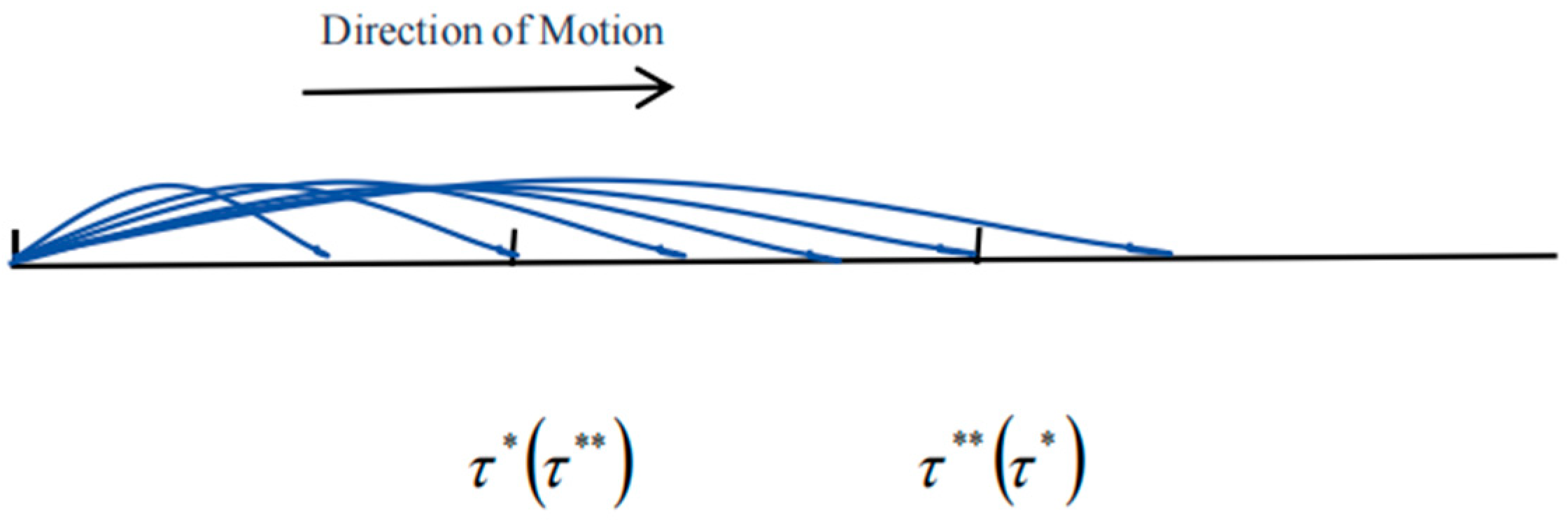
In the research problem of change point detection, Chen et al. [27] and Jia et al. [28] both utilized a method that gradually increases the length of the sliding window, as illustrated in Figure 1, for detecting change points. While this approach can effectively monitor structural change points in time series data, it has several limitations: (1) the critical value varies with the window length, complicating its determination; (2) it incurs high computational costs; (3) it is limited to identifying only a single type of change point and cannot distinguish mixed change points. Therefore, for the aforementioned mixed change-point model, this paper adopts a sliding monitoring method with a fixed window length to address the issue of change-point detection. The primary reasons for this choice are as follows: (1) the fixed-window sliding monitoring method overcomes the limitation of varying critical values by maintaining a constant threshold; (2) compared to the method with gradually increasing window lengths, the fixed-window approach significantly reduces computational load and cost; (3) the fixed-window sliding monitoring method can detect multiple types of change points and accurately identify their nature.
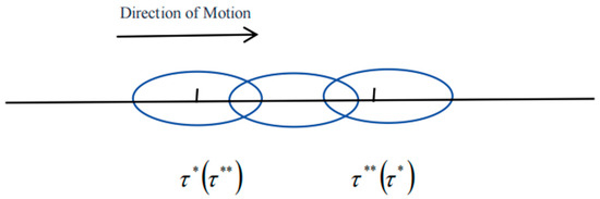
Figure 1.
A moving graph of the gradually increasing length of window frames.
Without loss of generality, let . There exists a non-unique such that and .
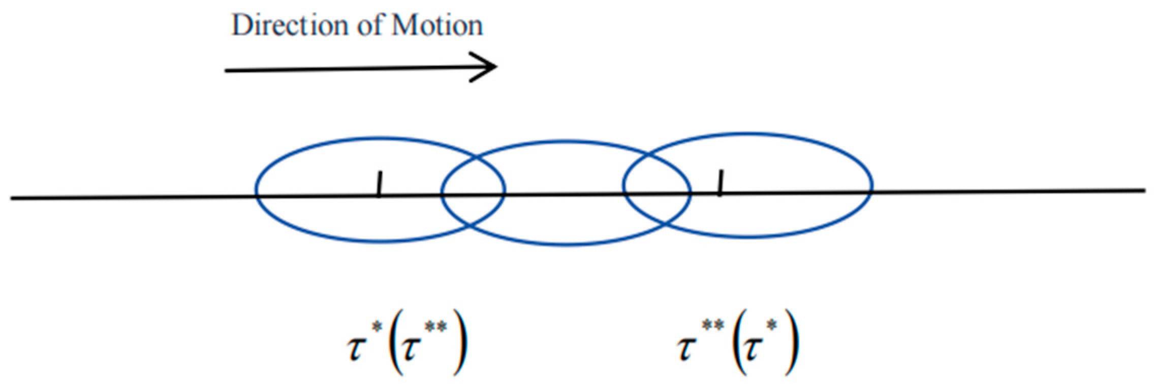
Additionally, there exist non-unique and , where h denotes the window-width parameter. Consequently, for a fixed h, the window width remains constant. During the hybrid change-point test, as the window frame slides along the data sequence, two scenarios may arise: (1) when , each window frame contains at most one change point, which can be either a variance change point or a mean change point. The movement of the window frame during the test process is illustrated in the following diagram (Figure 2).
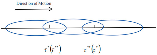
Figure 2.
When |τ* − τ**| > 2h, window frame movement diagram.
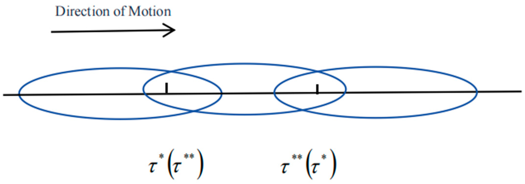
The second case occurs when . As the window frame moves along the data sequence, each window can contain at most two change points, which include the following scenarios: ① the window only covers the variance change point, ② the window only covers the mean change point, ③ the window covers both the variance change point and the mean change point. The diagram illustrating the movement of the window frame during the testing process is presented below (Figure 3).
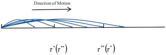
Figure 3.
When |τ* − τ**| < 2h, window frame movement diagram.
Assuming that satisfies condition (1), this paper addresses the hypothesis testing problem based on the relative positions of the mean change point and the variance change point.
The null hypothesis states that there are no change points in the sequence. The alternative hypothesis indicates that there is only a mean change point in the sequence. The alternative hypothesis suggests that there is only a variance change point in the sequence. The alternative hypothesis specifies that there are both mean and variance change points in the sequence, with no requirement for the moments of the mean change point and the variance change point to coincide.
Within the traditional cumulative sum (CUSUM) test framework, the limiting distribution properties of the test statistics are contingent upon the estimation of the long-term variance. Even if under the null hypothesis of no change point, it remains a significant challenge to obtain a consistent estimator for the long-term variance. In the more complex scenarios described by the alternative hypothesis, this estimation task becomes considerably more intricate. To mitigate the influence of the long-term variance on change-point detection, Horvath et al. [29] innovatively introduced ratio-type test statistics. By constructing the statistics in a ratio format, the impact of the long-term variance can be effectively neutralized. This approach not only circumvents the inherent difficulties associated with the long-term variance estimation but also enhances the theoretical conciseness and robustness of statistical inference in change-point detection. Thereby we adopt the ratio-type test to significantly improve the effectiveness of change-point detection.
Let . Upon the arrival of a new data point, the center of the window [ns] shifts rightward by one data point. Based on the residual sequence, we construct the following modified ratio-type test statistic:
where
and , ; , ; , .
Given that is unmeasurable, this paper conducts tests based on as a proxy for . The residual of is derived from regression analysis conducted on the intercept of .
2.2. Asymptotic Properties
First, derive the asymptotic distribution of the monitoring statistic under the null hypothesis.
Theorem 1.
Given that Assumptions 1–3 are satisfied, time series is generated according to Model (1). Under the null hypothesis , as , we have,
To achieve the objective of monitoring change points, we define the stopping time for detecting change points, where c denotes the critical value. Given the complexity of the asymptotic distribution of the statistic, we adopt the bootstrap sampling method. By conducting multiple resamplings, we can obtain a more precise critical value c.
The specific steps of the bootstrap sampling method are outlined as follows:
- Step 1: Compute the residuals
- Step 2: Center the residuals around zerocenter the residuals around zero:
- Step 3: For the 2[nh] method, bootstrap samples are randomly drawn from , and bootstrap samples are randomly drawn from , thereby forming .
- Step 4: Form the sequence . Similar to the construction of statistic , construct the statistic based on as follows:where
- Step 5: Repeat Steps 3 and 4 B times. Calculate the percentile, denoted as , of the resulting values. If , reject the null hypothesis, otherwise, do not reject it.
Theorem 2.
Under the null hypothesis and Assumptions 1–3, when , , , and under the conditions and , we have
The proof of the consistency of the statistics under the null hypothesis using the bootstrap sampling method follows a similar process to that outlined by Jin [30] et al. and Antoch [10]. Therefore, it will not be detailed here.
Theorem 3.
Under the conditions of Assumptions 1–3, the time series is generated by model (1). Under the alternative hypothesis , there exists a mean change point within a specified window, that is, there exists an index such that . In this study, we have
where
Theorem 4.
Under the conditions of Assumptions 1–3, the time series is generated by model (1). Under the alternative hypothesis , there exists a mean change point within a specified window, that is, there exists an index such that . In this study, we have
where
Theorem 5.
Under the conditions of Assumptions 1–3, the time series is generated by model (1). Under the alternative hypothesis , there exists a mean change point within a specified window, that is, there exists an index such that . In this study, we have
(The detailed proof process is presented in Appendix A).
3. The Updated Algorithm for Identifying Mixed Breakpoints
In this section, we estimate the positions of mean shift points and variance shift points, and eliminate the influence between shift points using an adjusted residuals method. This allows us to reconstruct the test statistics, thereby more accurately identifying the types of shift points.
According to Bai [11], the least squares estimator of the mean change-point can be derived using the following definition: , where , ; here, represents the sample mean of the first half of the [nr] observations, and represents the sample mean of the second half of the (n-[nr]) observations. Bai [14] demonstrated in his study on the least squares method for detecting mean change points in sequences of independent and identically distributed (i.i.d.) data that the convergence rate of the mean change-point estimator is assured. According to Bai’s proof, even in the presence of a variance change point, the accuracy of the mean change point estimator is maintained. But full proof is available on request.
The steps of the revised mixed change-point monitoring procedure are outlined as follows:
- Step 1: Compute the mean change-point estimator to mitigate the potential impact of variance change points, and subsequently set .
- Step 2: Based on the mean shift point time , calculate the means and for the first half and the second half , respectively. Then, .
- Step 3: Substitute into the statistical quantity to determine the nature of the change point. If no alarm is triggered, it indicates a mean change point. If an alarm is triggered, this can be further classified into two scenarios. The first scenario is a variance change point, representing a single change point. The second scenario involves the coexistence of mean and variance change points, indicating a compound change point.
- Step 4: Set and , then construct the variance change-point estimator , ensuring that .
- Step 5: Based on the identified time of the variance change point, calculate the variances and for the first half and the second half respectively. It is observed that .
- Step 6: Set ;
- Step 7: Substitute into the statistical quantity to determine the nature of the change point. If no alarm is triggered, it indicates a single change point characterized solely by variance variation; if an alarm is triggered, it implies the simultaneous occurrence of both mean and variance change points, indicating a dual-change-point scenario.
4. Monte Carlo Simulation
This section assesses the effectiveness of value-type statistics in detecting structural change points via Monte Carlo numerical simulations. The data generation process is described as follows:
- (1)
- When the mean change point precedes the variance change point,
- (2)
- When the variance change point precedes the mean change point,
Without loss of generality, let the significance level be denoted as , the monitoring sample size be , the uncontaminated sample size be , the window width be , the position of the mean change point be , the mean jump amplitude be , the position of the variance change point be , and the ratio of the standard deviations be . Table 1 provides the critical values for the test statistic . It is evident from Table 1 that the sample size of uncontaminated data has a relatively minor impact on the critical values and can be neglected. In contrast, both the sample size and the fixed window size significantly influence these critical values. Specifically, ① as the sample size increases, critical values decrease; ② as the fixed window size grows, critical values also decrease. Table 2 illustrates the empirical significance level of the test statistic at the 0.05 significance level, defined as the probability of rejecting the null hypothesis after 2000 repetitions of the experiment under the null hypothesis. It can be observed from the table that the significance level of the statistical quantity consistently hovers around 0.05. When the monitoring sample size is small and the window width is large, the number of window frames becomes relatively limited, leading to potential distortion. Conversely, when the monitoring sample size is large and the window width is small, the number of window frames increases substantially, resulting in a more conservative outcome. It can be inferred from Table 2 that empirical size relates to monitoring sample sizes, fixed window size, and uncontaminated sample sizes. To minimize deviations in empirical size, for small sample sizes, smaller window sizes and uncontaminated sample sizes should be used; for large sample sizes, larger window sizes should be employed while keeping smaller uncontaminated samples. This manifests specifically as follows: ① with an increase in monitoring sample size, there is a corresponding decrease in critical value; ② an increase in fixed window size results in a decrease in critical value.

Table 1.
The critical value of the test statistic Σ(s,r).
Table 2.
The significance level of the test statistic Σ(s,r) at the 0.05 significance level of the test.
Table 3 and Table 4 present the empirical power of the statistic under the hypotheses of mean breaks and variance breaks , respectively. The empirical power is defined as the rejection rate obtained from 2000 repeated trials under the alternative hypotheses. The following observations can be made from Table 3: ① when the window width remains constant and the monitoring sample size increases, the empirical power also increases, because the expanded window length captures more samples, which aligns with the findings of Theorem 2; ② the presence or absence of contamination in the sample size does not significantly affect the empirical power; ③ as anticipated, an increase in the mean jump amplitude leads to a corresponding increase in the empirical power; ④ since a moving window frame was selected in this study, the rejection rate remains insensitive to the position of the change point within the monitoring area. Regardless of whether the change point appears at the front or back of the entire sample, the moving window frame will inevitably cover it. For instance, given the monitoring sample size , the uncontaminated sample size , the window width , the jump amplitude , and the mean change-point position , the empirical potential is 0.8424; when the mean change point position is given, the empirical potential is 0.8185; and when the mean change-point position is given, the empirical potential is 0.8224. At this juncture, the empirical potential at the mean change-point position is greater than that at the mean change-point position ; ⑤ additionally, as the change point moves further away, the average run length decreases. This phenomenon may be attributed to the increased sliding number of the moving window frame and the subsequent testing of more samples when the change point is located further back. This conclusion aligns with the common principles governing change-point detection programs.
Table 3.
The test statistic Σ(s,r) is derived from the empirical power and ARL, assuming a mean shift as specified in the null hypothesis H1* (see details in the brackets).
Table 4.
The test statistic Σ(s,r) is derived from the empirical power and ARL, assuming a mean shift as specified in the null hypothesis H1** (see details in the brackets).
When only a variance change point is present, the aforementioned patterns can similarly be inferred from Table 4. For example, as the monitoring sample size increases, the empirical potential also increases; the sample size without contamination has minimal impact on the empirical potential; the rejection rate remains relatively insensitive to the position of the change point; and the average run length decreases when the change point occurs later in the sequence. Additionally, as the ratio of standard deviations increases, so does the empirical potential, indicating that the test statistic is particularly effective for detecting variance change points. For example, when the monitoring sample size is , the pollution-free sample size is , the window width is , the variance change-point position is , and the ratio of standard deviations is , the empirical potential equals 0.7255. When the ratio of standard deviations increases to , the empirical potential rises to 0.8761. This comparison confirms that the empirical potential is greater at a higher ratio of standard deviations than at a lower ratio . Therefore, it can be concluded that the proposed statistics exhibit superior performance in detecting both mean change points and variance change points.
Next, we examine the scenario involving mixed breakpoints. There are three distinct configurations for the window frame in relation to these breakpoints: (1) it covers only the mean breakpoint; (2) it covers only the variance breakpoint; (3) it simultaneously encompasses both the mean and variance breakpoints. To conserve space, the subsequent numerical simulations present results exclusively for a sample size of and a window width of . Under the assumption that all other parameters remain constant, by comparing the findings in Table 5 with those in Table 3 and Table 4, it becomes evident that ① the presence of a mean breakpoint induces a downward trend in the empirical power associated with the variance breakpoint. This decline is more pronounced when the magnitude of the mean jump is . For instance, when the monitoring sample size is , the mean breakpoint occurs at with a jump magnitude of , while the variance breakpoint is located at , resulting in a standard deviation ratio of and an empirical power of 0.3328. In contrast, when only the variance breakpoint exists, the empirical power is 0.7682. When all other conditions remain unchanged but the jump magnitude varies , the empirical power adjusts to 0.5231. ② Under the condition that other factors remain constant, when the ratio of standard deviations is negative, the decrease in empirical potential becomes more pronounced. For instance, with a monitoring sample size of , the mean change point located at , a jump amplitude of , the variance change point also at , and a ratio of standard deviations of , the empirical potential is 0.5231. In contrast, when only the variance change point exists, the empirical potential increases to 0.7760. Under identical conditions, when the ratio of standard deviations is , the empirical potential is 0.7682; however, when only the variance change point exists, it further increases to 0.8834. ③ When the mean change point is positioned further back, and the ratio of standard deviations is , the empirical potential decreases. This indicates that the presence of a mean change point weakens the test effect for the variance change point. Conversely, when the ratio of standard deviations is , the empirical potential increases, suggesting that the mean change point enhances the test effect for the variance change point. For example, with a monitoring sample size of , if the mean change point is located at , with a jump amplitude of , and the variance change point is at , while the ratio of standard deviations is , the empirical potential is 0.1916. However, in the absence of a mean change point, the empirical potential for only the variance change point is 0.6840. Under otherwise identical conditions, when the ratio of standard deviations is , the empirical potential rises to 0.8824, compared to 0.8050 when only the variance change point exists.
Table 5.
The test statistic Σ(s,r) is derived from the empirical power and ARL, assuming a mean shift as specified in the null hypothesis H1*** (see details in the brackets).
In conclusion, the concurrent presence of mean change points and variance change points can lead to distorted test outcomes. Therefore, this paper proposes a method for accurately identifying these change points. The detailed results are presented in Table 6 and Table 7. From Table 6, it is evident that the results and patterns after mean removal closely resemble those in Table 4. However, compared with Table 4, there remain some minor empirical potentials in Table 6, primarily due to the imprecise estimation of the positions of mean change points. In contrast to Table 5, the empirical potential in Table 6 has significantly increased. For instance, in Table 5, the position of the mean change point is , the mean jump amplitude is , the position of the variance change point is , and the ratio of standard deviations is , resulting in an empirical potential of 0.3328. Under otherwise identical conditions, the empirical potential obtained after mean removal is 0.7792. When only variance change points exist, the empirical potential is 0.7682. This indicates that the proposed method effectively mitigates the influence of mean change points on the detection of variance change points.
Table 6.
The empirical power and ARL of the test statistic Σ(s,r) after demeaning, under the assumption H1*** where both mean shift and variance shift coexist simultaneously, are examined.
Table 7.
The empirical power and ARL of the test statistic Σ(s,r) under the null hypothesis H1***, after variance adjustment and assuming simultaneous existence of both mean and variance change points, are evaluated as follows.
It can be observed from Table 7 that after removing the variance and reintroducing the trend, the results and patterns closely resemble those in Table 3. However, compared to Table 3, there are still some minor empirical potential differences in Table 7, primarily attributed to the underestimation of the variance change point. In contrast to Table 5, the empirical potential has significantly increased. For instance, in Table 5, the mean change point position is , the mean jump amplitude is , the variance change point position is , and the ratio of the standard deviation is , resulting in an empirical potential of 0.2647. Under otherwise identical conditions, after removing the variance and reintroducing the trend, the empirical potential increases to 0.8653. When only the mean change point exists, the empirical potential reaches 0.8840. These findings suggest that the proposed method effectively mitigates the impact of variance change points on the detection of mean change points.
By analyzing the aforementioned numerical simulation results, it is evident that the test outcomes become distorted when both mean change points and variance change points coexist. After correcting for the mean, an increased empirical potential value signifies the presence of variance change points; conversely, after correcting for the variance, an elevated empirical potential value indicates the existence of mean change points.
As shown in Table 2, the empirical size is approximately aligned with the nominal level 5%, which demonstrates that the Type I error is well controlled. Furthermore, Table 3, Table 4, Table 5, Table 6 and Table 7 reveal that the empirical power increases as a function of sample size, window width, jump amplitude, and standard deviation. For instance, in Table 3, when the monitoring sample size is , the window width is , the jump amplitude is , and the mean change point position is , the empirical power is 0.8863. This indicates that the probability of a Type II error is low. Consequently, the test methodology introduced in this paper exhibits strong control over both Type I and Type II errors.
5. Applications
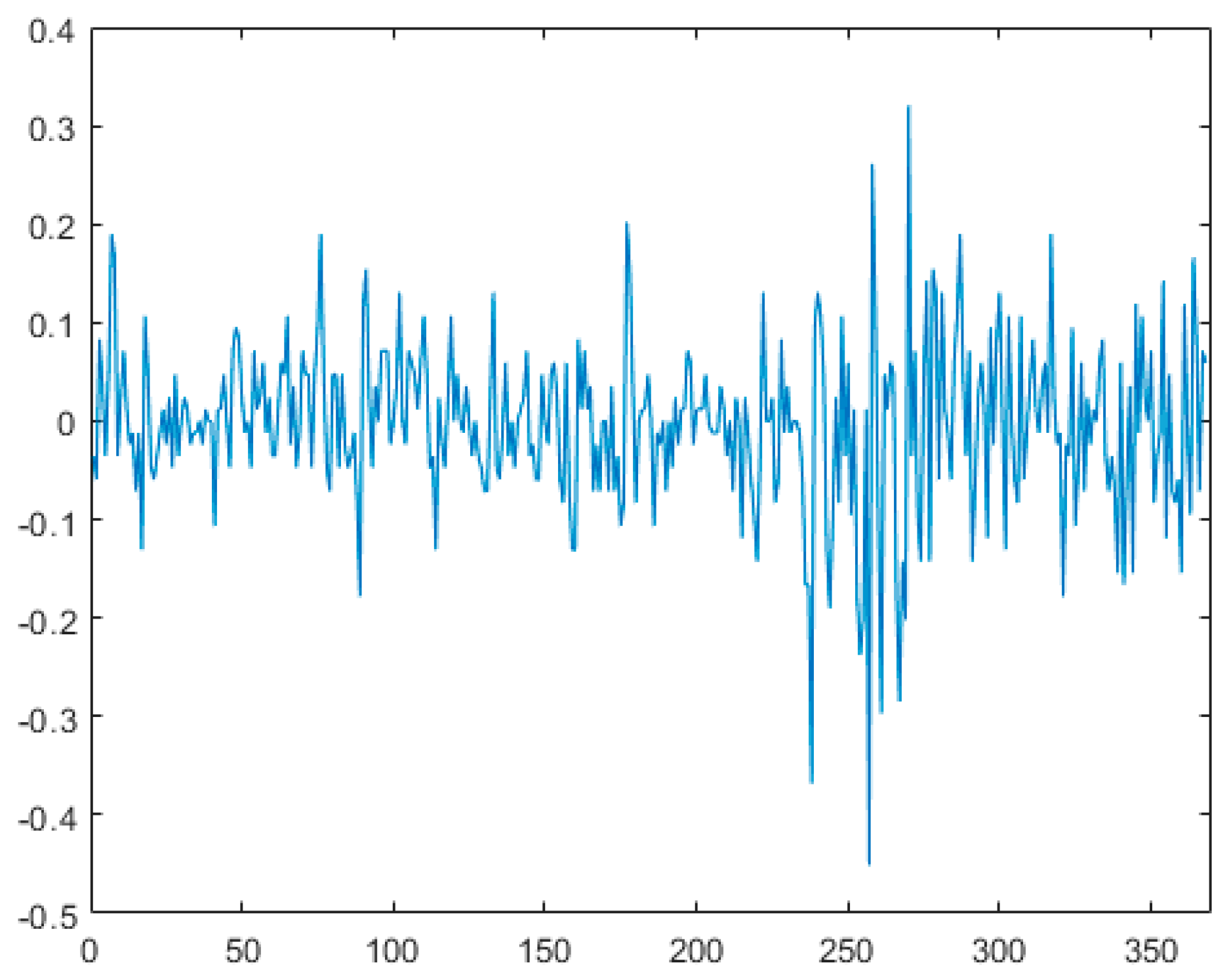
This section evaluates the effectiveness of the proposed method using the closing stock price data of IBM from 17 May 1961 to 2 November 1962, denoted as dataset . Figure 4 presents the scatter plot of the standardized dataset derived from , revealing a significant horizontal shift in the standardized sequence of these stock prices. This suggests the presence of a potential mean change point in the sequence. Figure 5 illustrates the first-order difference plot of the data, indicating volatility in the stock prices, leading us to suspect a variance change point in the sequence. In this analysis, the first 200 data points are treated as unpolluted data, with a window width . At a 5% significance level, we apply the variable change point monitoring method introduced in this paper, initiating the monitoring from the 201st observation to detect and classify any change points. (1) Dataset is substituted into variable , where , , to determine the estimated position of the mean change point. ① The sequence is divided into two segments, and . The sample mean of segment is calculated to be , while that of segment is . The data in each segment are then adjusted by subtracting their respective sample means, resulting in a new merged sequence . Upon re-monitoring, a change point is detected at the 238th sample. This change point may indicate either a variance change or both a variance and mean change. ② By computation, the sample variance of the first segment is , and that of the second segment is . After normalizing the data of both segments by their respective sample variances, we merged them into sequence for further monitoring. During this monitoring process, no change point was detected at the 238th sample. Consequently, it can be concluded that a variance change point exists at this position. (2) dataset was substituted into variable , where , , to determine the estimated position of the mean change point. The sequence was divided into two segments, designated as and . Calculations revealed that the sample mean of the first segment was , while that of the second segment was . The data from both segments were individually adjusted by subtracting their respective sample means, subsequently merged into a new sequence denoted as , and re-monitored. It was observed that no change point was detected at the 253rd sample. Consequently, it was concluded that only a mean change point existed at this position. This finding aligns with the results reported in Reference [31], demonstrating that the method proposed in this paper can not only effectively distinguish between mean change points and variance change points but also identify the type of change points more rapidly and accurately.
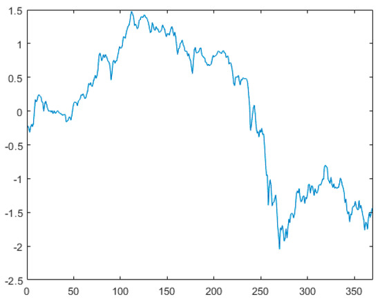
Figure 4.
Standardized data scatter plot.
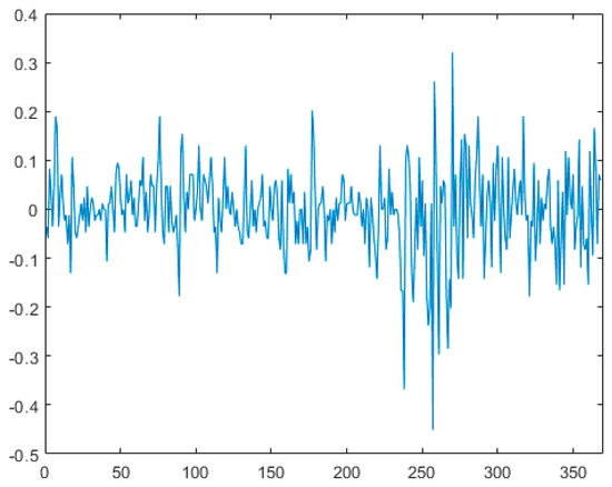
Figure 5.
First-order difference graph.
6. Conclusions
This paper investigates the issue of structural breaks within the time series mixed breakpoint model. By employing ratio-type statistics, the asymptotic distribution under the null hypothesis and consistency under the alternative hypothesis are rigorously derived. Additionally, a modified mixed breakpoint monitoring procedure is proposed. Through the application of residual adjustment methods, the influence between breaks is effectively eliminated, enabling the precise identification of break types. Numerical simulations indicate that the proposed method exhibits strong empirical performance and statistical power. In change point monitoring, it successfully distinguishes between mean change points and variance change points. Finally, using a real-world stock dataset, the practical feasibility and effectiveness of the proposed methodology are demonstrated.
Author Contributions
W.L.: writing—original draft, software; H.J.: methodology, writing—review and editing; M.W.: data curation, validation. All authors have read and agreed to the published version of the manuscript.
Funding
The authors would like to thank NNSF (Nos. 71473194), SNSF (Nos. 2020JM-513) for their financial support.
Data Availability Statement
The data presented in this article are derived from the Reference [32].
Conflicts of Interest
All authors disclose no conflicts of interest.
Appendix A
Proof of Theorem 1.
The residual sequence derived from
where , based on the definition of and the functional central limit theorem in conjunction with by Lemma 1, it follows that
Then, for molecules, there exists
First, address the second term in the denominator. Similarly, based on the residual sequences of , we observe that,
where , based on the definition of and Lemma 1, it follows that
and for the second term in the denominator, we find that
Similarly, concerning the first term in the denominator, we observe that,
By combining Equations (A1)–(A3), we arrive at the conclusion of Theorem 1.
Theorem 1 demonstrates that under the null hypothesis H0, the asymptotic distribution of the ratio-type test statistics introduced in this paper can be expressed as functional of Brownian motion. Through the construction of these ratio-type statistics, the need for estimating long-term variance is circumvented, thereby enhancing both the practicality and accuracy of the test. □
Proof of Theorem 3.
therefore,
this suggests that .
When , the change point occurs in the latter half of the sequence. This conclusion is drawn from the analysis of the residual sequence of ,
where , , according to the definition provided by and by Lemma 1, it can be inferred that
Then, for molecules, there exists
which suggests that .
When , that is, when the change point occurs in the latter half of the sequence, the second term of the denominator is influenced by this change point. In contrast, the first term of the denominator remains unchanged from its value under the null hypothesis and maintains a rate of . Therefore, for the first term of the denominator, we observe that it stays consistent with the null hypothesis at a rate of .
this suggests that .
For the second term in the denominator, based on the residual sequence , it can be observed that
where , .
- (i)
- When .
According to the definition provided by , it can be inferred that
- (ii)
- When , similarly,
Combining Equations (A4)–(A6) results in
By applying the same reasoning, we can demonstrate that , and consequently derive the following result:
The case where represents a special scenario for the change point position, meaning that the two segments are precisely divided at the exact moment of the change point. Following the same reasoning as in the preceding proof, in this situation, the first and second terms of the denominator remain unaffected by the change point, and their divergence rates align with the divergence rate of the denominator under the original hypothesis. However, the numerator continues to diverge, leading to a different behavior.
This suggests that . □
Proof of Theorem 4.
therefore,
this suggests that .
When , the change point occurs in the latter half of the sequence. This conclusion is drawn from the analysis of the residual sequence of ,
where , , .
According to the definition provided by and the functional central limit theorem in conjunction with , it can be inferred that
Then, for molecules, there exists
which suggests that .
When , that is, when the change point occurs in the latter half of the sequence, the second term of the denominator is influenced by this change point. In contrast, the first term of the denominator remains unchanged from its value under the null hypothesis and maintains a rate of . Therefore, for the first term of the denominator, we observe that it stays consistent with the null hypothesis at a rate of .
this suggests that .
For the second term in the denominator, based on the residual sequence , it can be observed that
where , .
- (i)
- When , similarly, it can be inferred that
- (ii)
- When , similarly,
Combining Equations (A7)–(A9) results in
By applying the same reasoning, we can demonstrate that , and consequently derive the following result:
The case where represents a special scenario for the change-point position, meaning that the two segments are precisely divided at the exact moment of the change point. Following the same reasoning as in the preceding proof, in this situation, the first and second terms of the denominator remain unaffected by the change point, and their divergence rates align with the divergence rate of the denominator under the original hypothesis. However, the numerator continues to diverge, leading to a different behavior.
This suggests that . □
Proof of Theorem 5.
Based on the proofs of Theorems 3 and 4, we primarily examine two cases: and . When , by analyzing the residual sequence of ,
where , ,
Similarly, it can be inferred that
Then, for molecules, there exists,
this suggests that .
When , the two segments divide precisely at the variance change point, which occurs prior to the mean change point. Consequently, the first term in the denominator remains unaffected by the change point, maintaining a divergence rate consistent with that under the null hypothesis. Therefore, for the first term of the denominator, it holds that
For the second term in the denominator, based on the residual sequence , it can be observed that
where , ,
- (i)
- When , similarly, it can be inferred that,
- (ii)
- When , similarly,
Therefore,
This indicates that . The divergence rate of the second term in the denominator is , leading to the conclusion that
It can be proved by the same reasoning that
In conclusion, . □
References
- Horváth, L.; Kokoszka, P.; Zhang, A. Monitoring constancy of variance in conditionally het-eroskedastic time series. Econ. Theory 2006, 22, 373–402. [Google Scholar] [CrossRef]
- Zhang, S.; Jin, H.; Su, M. Modified Block Bootstrap Testing for Persistence Change in Infinite Variance Observations. Mathematics 2024, 12, 258. [Google Scholar] [CrossRef]
- Jin, H.; Tian, S.; Hu, J.; Zhu, L.; Zhang, S. Robust ratio-typed test for location change under strong mixing heavy-tailed time series model. Commun. Stat.-Theory Methods 2025. [Google Scholar] [CrossRef]
- Zhang, X.; Jin, H.; Yang, Y. Quasi-autocorrelation coefficient change test of heavy-tailed sequences based on M-estimation. AIMS Math. 2024, 9, 19569. [Google Scholar] [CrossRef]
- Jin, H.; Hu, J.; Zhu, L.; Tian, S.; Zhang, S. M-Procedures Robust to Structural Changes Detection Under Strong Mixing Heavy-Tailed Time Series Models. J. Stat. Plan. Inference 2025. accepted. [Google Scholar] [CrossRef]
- Jin, H.; Wang, A.; Zhang, S.; Liu, J. Subsampling ratio tests for structural changes in time series with heavy-tailed AR(p) errors. Commun. Stat.-Simul. Comput. 2022, 53, 3721–3747. [Google Scholar] [CrossRef]
- Cavaliere, G. Unit root tests under time-varying variances. Econom. Rev. 2005, 23, 259–292. [Google Scholar] [CrossRef]
- Dette, H.; Wu, W.; Zhou, Z. Change point analysis of second order characteristics in non-stationary time series. arXiv 2015, arXiv:1503.08610. [Google Scholar]
- Long, C.X.; Chen, W.X.; Yang, R.; Yao, D.S. Ratio estimation of the population mean using auxiliary information under the optimal sampling design. Probab. Eng. Inf. Sci. 2022, 36, 449–460. [Google Scholar] [CrossRef]
- Antoch, J.; Hušková, M.; Veraverbeke, N. Change-point problem and bootstrap. J. Nonparametric Stat. 1995, 5, 123–144. [Google Scholar] [CrossRef]
- Bai, J. Least squares estimation of a shift in linear processes. J. Time Ser. Anal. 1994, 15, 453–472. [Google Scholar] [CrossRef]
- Inclán, C.; Tiao, G.C. Use of cumulative sums of squares for retrospective detection of change of variance. J. Am. Stat. Assoc. 1994, 89, 913–923. [Google Scholar]
- Gombay, E.; Horváth, L.; Hušková, M. Estimators and tests for change in variances. Stat. Decis. 1996, 14, 145–159. [Google Scholar] [CrossRef]
- Pitarakis, J.Y. Least squares estimation and tests of breaks in mean and variance under misspecification. Econometrics 2004, 7, 32–54. [Google Scholar] [CrossRef]
- Yuan, F.; Tian, Z.; Su, X.; Chen, Z. Cumulative Sum Estimation and Application of Mean and Variance Change Points in Independent Sequences. Control Theory Appl. 2010, 27, 395–399. [Google Scholar]
- Wang, H.; He, X.; Zhao, W. Estimation of Change Points of Mean and Variance for Dependent Sequences. J. Basic Sci. Text. Univ. 2017, 30, 75–80. [Google Scholar]
- Jin, H.; Zhang, J. Modified tests for variance changes in autoregressive regression. Math. Comput. Simul. 2011, 81, 1099–1109. [Google Scholar] [CrossRef]
- Jin, H.; Zhang, S.; Zhang, J.; Hao, H. Modified tests for change points in variance in the possible presence of mean breaks. J. Stat. Comput. Simul. 2018, 88, 2651–2667. [Google Scholar] [CrossRef]
- Aue, A. Strong approximation for RCA(1)time series with application. Stat. Probab. Lett. 2004, 68, 369–382. [Google Scholar] [CrossRef]
- Liu, W.; Liu, J.; Qin, R. Online monitoring of change points for multivariate normal vectors. J. Shanxi Univ. (Nat. Sci. Ed.) 2015, 38, 475–496. [Google Scholar]
- Horvath, L.; Kuhn, M.; Steinebach, J. On the performance of the fluctuation test for structural change. Seq. Anal. 2008, 27, 126–140. [Google Scholar] [CrossRef]
- Aue, A.; Horváth, L.; Kühn, M.; Steinebach, J. On the reaction time of moving sum detectors. J. Stat. Plan. Inference 2012, 142, 2271–2288. [Google Scholar] [CrossRef]
- Qi, P.; Tian, Z.; Duan, X. Sequential Monitoring Variance Changes in Location Model. Commun. Stat.-Theory Methods 2015, 44, 5267–5284. [Google Scholar] [CrossRef]
- Zhao, W.; Xia, Z.; Tian, Z. Ratio test to detect change in the variance of linear process. Statistics 2011, 45, 189–198. [Google Scholar] [CrossRef]
- Qin, R.; You, Y. A ratio test for variance change points in linear processes. Henan Sci. 2020, 38, 33–40. [Google Scholar]
- Davidson, J.E.H. Stochastic Limit Theory, 2nd ed.; Oxford University: Oxford, UK, 1995. [Google Scholar]
- Chen, Z.; Li, F.; Zhu, L.; Xing, Y. Monitoring mean and variance change-points in long-memory time series. J. Syst. Sci. Complex. 2022, 35, 1009–1029. [Google Scholar] [CrossRef]
- Jia, W.; Wei, Y.; Xu, J. Online Monitoring of Mean Change Points in RCA(1) Time Series Model. J. Huaibei Norm. Univ. (Nat. Sci. Ed.) 2023, 44, 1–9. [Google Scholar]
- Horváth, L.; Horváth, Z.; Hušková, M. Ratio tests for change point detection. Inst. Math. Stat. Collect. 2008, 1, 293–304. [Google Scholar]
- Jin, H.; Tian, Z.; Qin, R.B. Bootstrap tests for structural change with infinite variance observations. Stat. Probab. Lett. 2009, 79, 1985–1995. [Google Scholar] [CrossRef]
- Chen, Z.; Tian, Z.; Ding, M. Online Monitoring of Parameter Change Points in Linear Regression Models. Syst. Eng.-Theory Pract. 2010, 30, 1047–1054. [Google Scholar]
- Box, G.E.P.; Jenkins, G.M.; Reinsel, G.C. Time Series Analysis: Forecasting and Control, 3rd ed.; Prentice Hall: Englewood Cliffs, NJ, USA, 1994. [Google Scholar]

Disclaimer/Publisher’s Note: The statements, opinions and data contained in all publications are solely those of the individual author(s) and contributor(s) and not of MDPI and/or the editor(s). MDPI and/or the editor(s) disclaim responsibility for any injury to people or property resulting from any ideas, methods, instructions or products referred to in the content. |
© 2025 by the authors. Licensee MDPI, Basel, Switzerland. This article is an open access article distributed under the terms and conditions of the Creative Commons Attribution (CC BY) license (https://creativecommons.org/licenses/by/4.0/).