Data-Driven Robust Attitude Tracking Control of Unmanned Underwater Vehicles with Performance Constraints

Abstract

This paper studies the data-driven attitude tracking control issue for an unmanned underwater vehicle (UUV) with disturbances. First, a new polynomial finite-time prescribed performance function (FTPF) is introduced to avoid the problem of the computation number increasing as the exponential term increases in the conventional exponential FTPF. By using the new polynomial FTPF, the tracking error is converted into a constrained form. Then, an estimator is designed for estimating the unknown pseudo-partitioned Jacobian matrix (PJM) in the linearization model, and a discrete-time nonlinear disturbance observer (DNDO) is adopted for observing unknown disturbances. It is worth noting that the DNDO can avoid the large overshoot by introducing a saturated function. With the help of the estimator for the PJM, the DNDO, and the constrained error, a data-driven robust control strategy with performance constraints is designed to fulfill accurate attitude tracking control of the UUV, which ensures that the tracking error draws into a prescribed region in a predetermined time. Eventually, the control strategy is verified by numerical simulations.

1. Introduction

In recent years, the attitude tracking control of unmanned underwater vehicles (UUVs) has attracted substantial attention due to its widespread applications in various underwater tasks, including terrain imaging, underwater detection, and object monitoring, among others. As a result, numerous significant advancements [1,2,3,4,5] have been made in the attitude tracking control area of UUVs. Notably, during actual underwater tasks, a UUV exhibits a high coupling and strong nonlinearity, which raises the problem that the accurate UUV model is difficult to obtain. Fortunately, data-driven control offers a viable approach without involving a system model; for example, the discrete-time proportional–integral–derivative control in [6], iterative learning control in [7,8,9], lazy learning control in [10], etc. As a data-driven solution, model-free adaptive control (MFAC) in [11] has recently emerged as a promising approach because of its convenient adjustment, computational simplicity, better robustness, etc. Through continuous development, MFAC has been widely used in various fields in [12,13,14,15,16]. Note that, although most MFAC-based control schemes can guarantee system stability, control performance cannot be prescribed.

To ensure that control performance can be prescribed, prescribed performance control (PPC) provides a powerful method for this in [17] by taking a performance function. After that, some representative schemes are studied. In [18], a PPC-based robust controller is designed for linear systems, and then the controller is adopted for nonlinear systems in [19]. In [20], a PPC-based fault-tolerant controller is designed with guaranteed prescribed bounds and zero overshoot, and a data-driven control scheme with performance constraints is designed in [21]. In [22], a preset trajectory controller is presented for a vehicle system. Nevertheless, the above PPC-based methods can only ensure that the error converges to a prescribed region in an infinite time. To make it so that the time can be predetermined, a finite-time prescribed performance function (FTPF) is introduced in [23,24]. In [25], a finite-time PPC-based adaptive fuzzy control algorithm is proposed for strict-feedback systems. With the aid of an FTPF, a consensus control strategy is proposed for multiple systems in [26]. Note that the above FTPF operates in an exponential form, where the computation number increases as the exponential term increases, leading to an increase in the computation complexity. Additionally, for the current error transformation function in [17,21], a singularity problem is generated since the denominator has a negative sign, which may severely affect system stability. Therefore, it is important to consider a new FTPF to reduce the computation burden and design a modified error transformation function to avoid the singularity problem.

What is more, disturbances inevitably occur during the operation of UUVs, which are usually caused by marine environmental factors, communication signal anomalies, magnetic field changes, navigation errors, etc., leading to a performance reduction of the UUVs. Due to this challenge, precise attitude tracking of UUVs has become a formidable task, and a variety of anti-disturbance control strategies have been proposed, such as adaptive control in [27], fuzzy control in [28], and sliding mode control in [29], etc. As an anti-disturbance control approach, a disturbance observer in [30] is widely used to offset the negative influence of disturbances. For example, a robust control scheme based on a linear disturbance observer is proposed in [31]. Then, a nonlinear disturbance observer using time-varying gain is developed in [32], and a comprehensive stability analysis is provided in [33]. However, the aforementioned schemes can only be observed for an infinite period of time. To realize finite-time observation, a finite-time disturbance observer is developed to fulfill the stable control for the telecontrolled robotic manipulators in [34]. Furthermore, a cascade disturbance observer in [35] is used for the attenuation of current disturbances. However, the above control strategy only applies to continuous systems and is not applied in discrete-time systems. In addition, the above results all require an assumption that the system model is known. In order to solve the problem, a discrete-time linear disturbance observer in [36] is explored without involving a system model. However, the large overshoot tends to occur when the observed gain is large. Therefore, it is necessary to adopt a discrete-time nonlinear disturbance observer (DNDO) to avoid the large overshoot.

As far as we know, there is little research about the data-driven attitude tracking control issue of UUVs without involving system models. Moreover, few results adopt data-driven robust control methods with performance constraints. Inspired by the above discussions, a data-driven robust attitude tracking control strategy with performance constraints is proposed for UUVs. The principal innovations are demonstrated below:

(i)

In comparison to most FTPFs in [23,25,26] operating with an exponential form, where the computation number increases as the exponential term increases, a new polynomial FTPF is adopted in this paper, where the calculation number of the polynomial FTPF is invariable, effectually reducing the computation burden. Additionally, different from the traditional error transformation function in [17,21], which causes a singularity problem since the denominator has a negative sign, a new transformed function is adopted to avoid the singularity problem in the error transformation.

(ii)

In contrast to the current results in [30,31,32,33,34] involving the system model, the constructed disturbance observer only uses data information without involving system models. In addition, different from the disturbance observer in [36], where the large overshoot tends to occur when the observed gain is large, a DNDO from [16] is adopted in this paper to avoid the large overshoot by introducing a saturated function.

(iii)

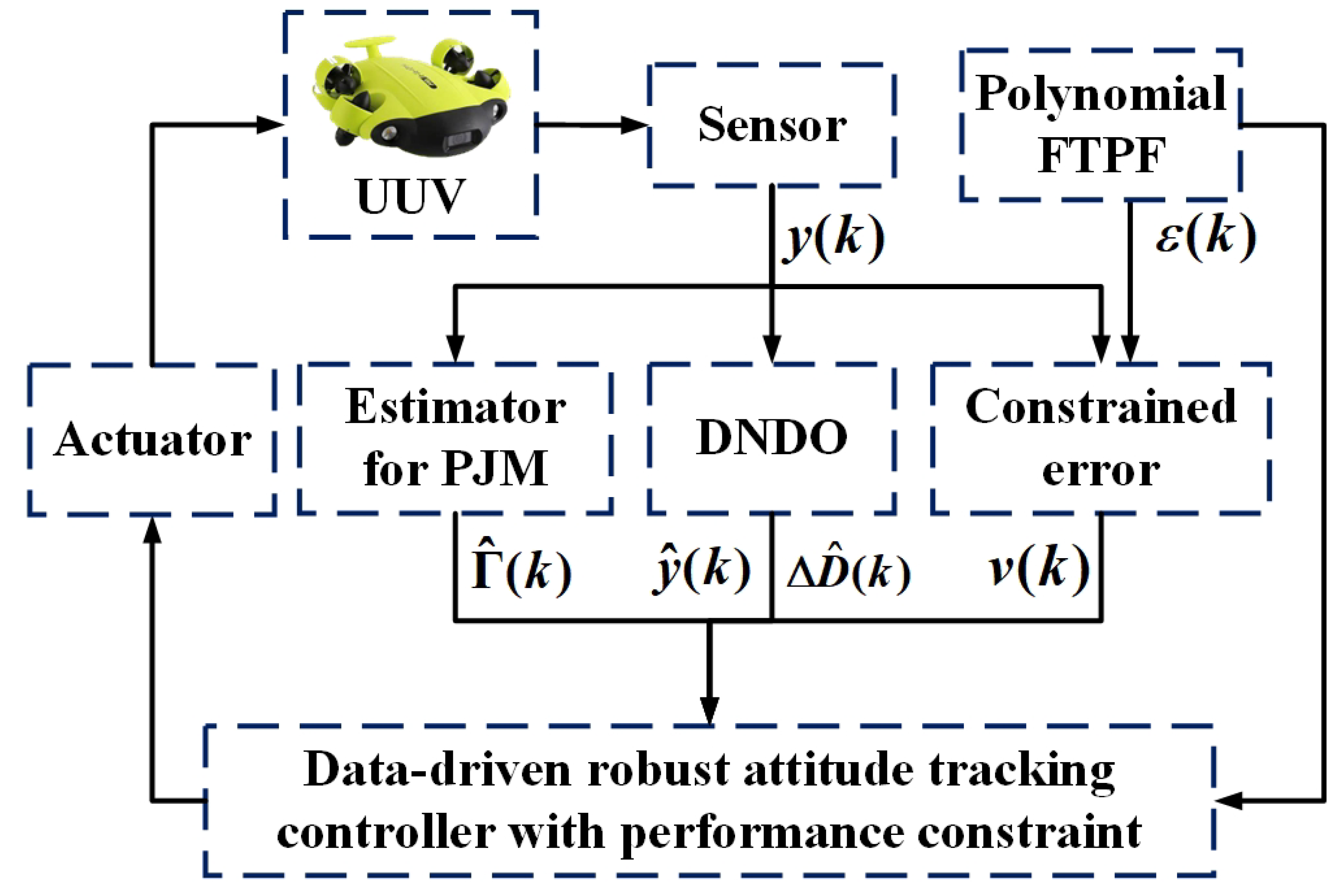
By means of the constrained error and the DNDO, a data-driven robust control strategy with performance constraints is designed to fulfill accurate attitude tracking control of UUVs, which ensures that the error draws into a prescribed region in a predetermined time.

This paper is formatted below as follows: Section 1 presents the introduction. Section 2 provides the notation, the system model, and the control target. Section 3 designs the data-driven robust control strategy with performance constraints and provides stability analysis. Section 4 outlines the simulations. Section 5 comprises the conclusion.

2. Problem Statement

2.1. Notation

$\mathbb{R}$ represents a real number, ${\mathbb{R}}^n$ represents a real vector, and ${\mathbb{R}}^{n\times n}$ represents a real matrix. $\parallel ·\parallel$ represents a Euclidean norm or 2-norm. $\mathrm{T}$ represents the transposition symbol. For the $\mathit{x}={[x_1,x_2,\dots ,x_n]}^T\in {\mathbb{R}}^n$, its norm is $\parallel \mathit{x}\parallel =\sqrt{{\mathit{x}}^T\mathit{x}}$. For the $\mathit{A}\in {\mathbb{R}}^{n\times n}$, its norm is $\parallel \mathit{A}\parallel =\sqrt{({\mathit{A}}^T\mathit{A})}$. $\mathrm{sign}$ is a sign function. $\exp (·)$ is an exponential function with a base of e. $\mathit{I}\in {\mathbb{R}}^n$ represents an identity vector. ${\mathit{I}}_n\in {\mathbb{R}}^{n\times n}$ represents an identity matrix. For the vector $\mathit{x}=[x_1,x_2,x_3]\in {\mathbb{R}}^3$, there is

$${\mathit{x}}^{\times }=\left[\begin{array}{ccc}0& -x_3& x_2\\ x_3& 0& -x_1\\ -x_2& x_1& 0\end{array}\right].$$

2.2. System Model

This paper considers two UUVs, and the attitude tracking control framework is displayed in Figure 1, which includes a body reference frame ${\mathcal{R}}_b$ of the follower, the desired reference frame ${\mathcal{R}}_d$ of the leader, and the earth reference frame ${\mathcal{R}}_e$.

The system model of the leader is constructed by Euler angle as

$$\begin{array}{cc}\hfill & {\dot{\mathbf{\Theta }}}_d=\mathit{W}{\mathit{\omega }}_d,\hfill \\ \hfill & {\mathit{J}}_d{\dot{\mathit{\omega }}}_d=-{{\mathit{\omega }}_d}^{\times }{\mathit{J}}_d{\mathit{\omega }}_d+{\mathit{S}}_d{\mathit{\omega }}_d,\hfill \end{array}$$

(1)

where ${\mathbf{\Theta }}_d=[{\varphi }_d$${\theta }_d$${\psi }_d{]}^T\in {\mathbb{R}}^3$ denotes the attitude of the leader, where ${\varphi }_d$, ${\theta }_d$, and ${\psi }_d$ are the yaw, pitch, and roll angles of the leader, ${\mathit{\omega }}_d=[{\omega }_d^{\varphi }$${\omega }_d^{\theta }$${\omega }_d^{\psi }{]}^T\in {\mathbb{R}}^3$ denotes the angular velocity of the leader, ${\mathit{J}}_d\in {\mathbb{R}}^{3\times 3}$ denotes the inertial matrix, ${\mathit{S}}_d\in {\mathbb{R}}^{3\times 3}$ denotes the predefined constant matrix.

The system model of the follower is constructed by Euler angle as

$$\begin{array}{cc}\hfill & \dot{\mathbf{\Theta }}=\mathit{W}\mathit{\omega },\hfill \\ \hfill & \mathit{J}\dot{\mathit{\omega }}=-{\mathit{\omega }}^{\times }\mathit{J}\mathit{\omega }+\mathit{L}+\mathit{u}+\mathit{d},\hfill \end{array}$$

(2)

where $\mathbf{\Theta }=[\varphi$$\theta$${\psi ]}^T\in {\mathbb{R}}^3$ denotes the attitude of the follower, where $\varphi$, $\theta$, and $\psi$ are the yaw, pitch, and roll angles of the follower, $\mathit{\omega }=[{\omega }^{\varphi }$${\omega }^{\theta }$${\omega }^{\psi }{]}^T\in {\mathbb{R}}^3$ denotes the angular velocity of the follower, $\mathit{J}\in {\mathbb{R}}^{3\times 3}$ denotes the inertial matrix, $\mathit{L}=[l_1$$l_2$$l_3{]}^T\in {\mathbb{R}}^3$ denotes the lumped force received by the follower with $\mathit{L}=-\mathit{C}(\mathit{\omega })\mathit{\omega }-\mathit{G}(\mathit{\omega })\mathit{\omega }+\mathit{M}+\mathit{F}$, where $\mathit{C}(\mathit{\omega })\in {\mathbb{R}}^{3\times 3}$ denotes the coriolis matrix, $\mathit{G}(\mathit{\omega })\in {\mathbb{R}}^{3\times 3}$ denotes the damping matrix, $\mathit{M}\in {\mathbb{R}}^3$ denotes the heavy torque, and $\mathit{F}\in {\mathbb{R}}^3$ denotes the floating torque, $\mathit{u}=[u_1$$u_2$$u_3{]}^T\in {\mathbb{R}}^3$ denotes the control torque generated by the propulsion system of the UUV, and $\mathit{d}=[d_1$$d_2$$d_3{]}^T\in {\mathbb{R}}^3$ denotes various disturbances that the UUV may be subjected to when performing the task, which are usually caused by marine environmental factors, communication signal anomalies, magnetic field changes, navigation errors, etc.

The system output of the UUV is $\mathit{y}={\mathit{C}}_1\mathbf{\Theta }+{\mathit{C}}_2\mathit{\omega }$, and the desired output is ${\mathit{y}}_d={\mathit{C}}_1{\mathbf{\Theta }}_d+{\mathit{C}}_2{\mathit{\omega }}_d$, where ${\mathit{C}}_1\in {\mathbb{R}}^{3\times 3}$ and ${\mathit{C}}_2\in {\mathbb{R}}^{3\times 3}$ are adjustable diagonal matrices. The system and desired output at the $(k+1)$th moment are presented as

$$\left\{\begin{array}{c}\mathit{y}(k+1)={\mathit{C}}_1\mathbf{\Theta }(k+1)+{\mathit{C}}_2\mathit{\omega }(k+1),\hfill \\ {\mathit{y}}_d(k+1)={\mathit{C}}_1{\mathbf{\Theta }}_d(k+1)+{\mathit{C}}_2{\mathit{\omega }}_d(k+1).\hfill \end{array}\right.$$

(3)

Based on (1)–(3), the $\mathit{y}(k+1)$ is written as an autoregression model [11]

$$\begin{array}{cc}\hfill & \mathit{y}(k+1)=\mathit{L}\{\mathit{y}(k),\mathit{u}(k)\}+\mathit{D}(k),\hfill \end{array}$$

(4)

where $\mathit{L}\{·\}$ is a nonlinear function about $\mathit{y}(k)$ and $\mathit{u}(k)$, and $\mathit{D}(k)={\mathit{C}}_2{\mathit{J}}^{-1}\mathit{d}(k)$ is the lumped disturbances.

Assumption 1. 

For the leader, ${\mathit{J}}_d{\dot{\mathit{\omega }}}_d=-{{\mathit{\omega }}_d}^{\times }{\mathit{J}}_d{\mathit{\omega }}_d+{\mathit{S}}_d{\mathit{\omega }}_d$ is stable.

Assumption 2. 

The disturbances encountered by the UUV are bounded during the execution of tasks, i.e., $\parallel \mathit{d}\parallel \le \overline{d}$ with $\overline{d}$ being an unknown but bounded constant.

Assumption 3. 

$\mathit{L}\{·\}$ to $\mathit{y}(k)$ and $\mathit{u}(k)$ has continuous partial derivatives, the system (4) meets the Lipschitz condition, and $\parallel \Delta \mathit{y}(k+1)\parallel \le \gamma \parallel \Delta \mathit{H}(k)\parallel$ with $\Delta \mathit{H}(k)={[\Delta \mathit{y}(k),\Delta \mathit{u}(k)]}^{\mathrm{T}}$, where $\Delta \mathit{y}(k)=\mathit{y}(k)-\mathit{y}(k-1)$, $\Delta \mathit{u}(k)=\mathit{u}(k)-\mathit{u}(k-1)$, and $\gamma >0$ is a bounded constant.

Lemma 1 

([11]). For the system (4), if Assumptions 1–2 hold, there exists an unknown pseudo-partitioned Jacobian matrix (PJM) $\mathbf{\Gamma }=[{\mathbf{\Gamma }}_1,{\mathbf{\Gamma }}_2]\in {\mathbb{R}}^{3\times 6}$ such that the system (4) is constructed as

$$\begin{array}{c}\hfill \Delta \mathit{y}(k+1)=\mathbf{\Gamma }(k)\Delta \mathit{H}(k)+\Delta \mathit{D}(k),\end{array}$$

(5)

where $\parallel \mathbf{\Gamma }(k)\parallel \le \gamma$ with γ being an unknown but bounded constant, and $\Delta \mathit{D}(k)=\mathit{D}(k)-$$\mathit{D}(k-1)$.

Assumption 4. 

The symbol of block matrix ${\mathbf{\Gamma }}_2(k)$ in (5) remains unchanged, which means that the control direction is known or invariant, and ${\mathbf{\Gamma }}_{i,2,pq}(k)\le {\kappa }_1$, ${\kappa }_2\le {\mathbf{\Gamma }}_{i,2,pp}(k)\le \sigma {\kappa }_2$, $p,q=1,\dots ,3$, where $\sigma \ge 1$ and ${\kappa }_2>2{\kappa }_1(2\sigma +1)$ are bounded constants.

Remark 1. 

Assumption 1 is a conventional hypothesis in the model-free adaptive control (MFAC) [11]. Assumption 2 is reasonable and conforms to the actual situation. Assumption 3 is a “linear-like” condition, which means the output increments are constrained by the input increment [12]. Lemma 1 is adopted to change the system in (4) into a linear system. Additionally, since only the data information can be available, Assumption 4 is a viable option to describe the coupling between input variables [13].

2.3. Control Target

To describe the attitude tracking control target, the error is described as

$$\begin{array}{c}\hfill \mathit{e}(k)={\mathit{y}}_d(k)-\mathit{y}(k),\end{array}$$

(6)

where $\mathit{e}(k)=[e_1(k)$$e_2(k)$$e_3{(k)]}^T\in {\mathbb{R}}^3$, and ${\mathit{y}}_d(k)$ and $\mathit{y}(k)$ are defined in (3).

Our aim is to design a data-driven robust control strategy with performance constraints such that the tracking error $\mathit{e}(k)$ draws into a prescribed region in a predetermined time, i.e.,

$$\left\{\begin{array}{ccc}-{\phi }_l\epsilon (k)<e_p(k)<{\phi }_h\epsilon (k),\hfill & \hfill & \mathrm{if}[0,k_f),\hfill \\ -{\phi }_l\epsilon (k_f)<e_p(k)<{\phi }_h\epsilon (k_f),\hfill & \hfill & \mathrm{if}[k_f,\infty ),\hfill \end{array}\right.$$

(7)

where $e_p(k)$, $p=1,\dots ,3$, denotes the component of the $\mathit{e}(k)$ in (6), ${\phi }_l>0$ and ${\phi }_h>0$ are design parameters, $\epsilon (k)$ denotes the performance function in (10), and $k_f$ denotes the predetermined time.

3. Control Strategy Design

First, a finite-time prescribed performance function (FTPF) with a polynomial form is presented, and the error $\mathit{e}(k)$ is converted into a constrained form. In addition, an estimator is designed for estimating the PJM in the linearization model (5), and a discrete-time nonlinear disturbance observer (DNDO) is adopted to offset the negative effect of disturbances. By using the estimator for the PJM, the DNDO, and the constrained error, a data-driven robust attitude tracking control strategy with performance constraints is developed for UUVs. The block diagram is shown in Figure 2.

3.1. Polynomial FTPF and Error Transformation

In most PPC-based methods [17,18,19,20,21], the performance function is set as

$$\begin{array}{c}\hfill {\epsilon }_{old}(k)=({\epsilon }_{old,0}-{\epsilon }_{old,\infty })exp(-{\vartheta }_{old}k)+{\epsilon }_{old,\infty },\end{array}$$

(8)

where ${\epsilon }_{old,0}>{\epsilon }_{old,\infty }>0$ and ${\vartheta }_{old}>0$ are adjustable parameters.

Note that the convergence time of the ${\epsilon }_{old}(k)$ is not predetermined and changes with the design parameters. To meet the requirement that the convergence time is predetermined, the FTPF is set as

$${\epsilon }_{old}^f(k)=\left\{\begin{array}{cccc}\hfill ({\epsilon }_{old,0}^f-{\epsilon }_{old,\infty }^f)exp({\displaystyle \frac{-{\vartheta }_{old}^f{k}_{f}k}{k_f-k}})+{\epsilon }_{old,\infty }^f,& \hfill & & k\in [0,k_f),\hfill \\ \hfill {\epsilon }_{old,\infty }^f,& \hfill & & k\in [k_f,\infty ),\hfill \end{array}\right.$$

(9)

where ${\epsilon }_{old,0}^f>{\epsilon }_{old,\infty }^f>0$ and ${\vartheta }_{old}^f>0$ are adjustable parameters, and $0<k_f<\infty$ represents the predetermined time.

Although the ${\epsilon }_{old}^f(k)$ meets the requirement that the convergence time is predetermined in [23,25,26], it operates in an exponential form, where the computation number increases as the exponential term k increases, leading to an increase in the computation complexity. Thus, a new FTPF with a polynomial form is set as

$$\epsilon (k)=\left\{\begin{array}{cccc}\hfill l_3{k}^3+l_2{k}^2+l_{1}k+{\epsilon }_0,& \hfill & & k\in [0,k_f),\hfill \\ \hfill {\epsilon }_{\infty },& \hfill & & k\in [k_f,\infty ),\hfill \end{array}\right.$$

(10)

where $l_1$, $l_2$, $l_3$, ${\epsilon }_0$, and ${\epsilon }_{\infty }$ are adjustable parameters satisfying

$$\left\{\begin{array}{c}\epsilon (0)={\epsilon }_0,\hfill \\ \epsilon (k_f)=l_3{k}_f^3+l_2{k}_f^2+l_1{k}_f+l_0={\epsilon }_{\infty },\hfill \\ \dot{\epsilon }(k_f)=3l_3{k}_f^2+2l_2{k}_f+l_1=0,\hfill \\ \ddot{\epsilon }(k_f)=6l_3{k}_f+2l_2=0.\hfill \end{array}\right.$$

(11)

Based on (11), $l_1$, $l_2$, and $l_3$ are solved as

$$\left\{\begin{array}{c}{l}_1=-3({\epsilon }_0-{\epsilon }_{\infty })/k_f,\hfill \\ l_2=3({\epsilon }_0-{\epsilon }_{\infty })/k_f^2,\hfill \\ l_3=-3({\epsilon }_0-{\epsilon }_{\infty })/k_f^3.\hfill \end{array}\right.$$

(12)

Note that in the control target (7), the tracking error $e_p(k)$ satisfies

$$\left\{\begin{array}{ccc}-{\phi }_l\epsilon (k)<e_p(k)<{\phi }_h\epsilon (k),\hfill & \hfill & \mathrm{if}[0,k_f),\hfill \\ -{\phi }_l\epsilon (k_f)<e_p(k)<{\phi }_h\epsilon (k_f),\hfill & \hfill & \mathrm{if}[k_f,\infty ),\hfill \end{array}\right.$$

(13)

Since this control target in (7) is difficult to achieve, an auxiliary variable $\overline{\mathit{e}}(k)=[{\overline{e}}_1(k)$${\overline{e}}_2(k)$${\overline{e}}_3{(k)]}^T\in {\mathbb{R}}^3$ by means of the polynomial FTPF in (10) is introduced as

$$\begin{array}{c}\hfill {\overline{e}}_p(k)={\displaystyle \frac{2}{{\phi }_l+{\phi }_h}}\left({\displaystyle \frac{e_p(k)}{\epsilon (k)}}-{\displaystyle \frac{{\phi }_h-{\phi }_l}{2}}\right),p=1,\dots ,3,\end{array}$$

(14)

where ${\phi }_l>0$ and ${\phi }_h>0$ are adjustable parameters.

Based on (13), we have

$$\begin{array}{c}\hfill -1<{\overline{e}}_p(k)<1.\end{array}$$

(15)

To achieve (14), the error transformation is introduced as

$$\begin{array}{c}\hfill {\overline{e}}_p(k)=\mathbf{\Xi }(v_p(k)),\end{array}$$

(16)

where $e_p(k)$ is the component of $\mathit{e}(k)$ in (6), $\mathit{v}(k)=[v_1(k)$$v_2(k)$$v_3{(k)]}^T\in {\mathbb{R}}^3$ is the constrained error with the components $v_p(k)$, $p=1,\dots ,3$, and $\mathbf{\Xi }(v_p(k))$ is a monotonic function satisfying

$$\left\{\begin{array}{c}\mathbf{\Xi }(v_p(k))\in (-1,1),\hfill \\ \mathbf{\Xi }(v_p(k))=1,\mathrm{if}{v}_p(k)\to +\infty ,\hfill \\ \mathbf{\Xi }(v_p(k))=-1,\mathrm{if}{v}_p(k)\to -\infty .\hfill \end{array}\right.$$

(17)

By means of (17), there must exist ${\mathbf{\Xi }}^{-1}(v_p(t))$ such that $v_p(k)={\mathbf{\Xi }}^{-1}({\overline{e}}_p(k))$. According to Condition (17), the conventional transformation function is usually set as [17,21]

$$\begin{array}{c}\hfill {\mathbf{\Xi }}_{old}(v_p(k))={\displaystyle \frac{exp({\overline{e}}_p(k))-exp(-{\overline{e}}_p(k))}{exp({\overline{e}}_p(k))+exp(-{\overline{e}}_p(k))}},\end{array}$$

(18)

and the constrained error $v_p(k)$ is changed to

$$\begin{array}{c}\hfill v_p(k)={\displaystyle \frac{1}{2}}ln({\displaystyle \frac{1+{\overline{e}}_p(k)}{1-{\overline{e}}_p(k)}}).\end{array}$$

(19)

Note that a singularity problem is produced when ${\overline{e}}_p(k)=1$, which may severely affect system stability. To avoid the singularity problem, a new error transformation function is set as

$$\begin{array}{c}\hfill {\mathbf{\Xi }}_{new}(v_p(k))={\displaystyle \frac{2}{\pi }}arctan({\overline{e}}_p(k)).\end{array}$$

(20)

Based on (20), the constrained error $v_p(k)$ is rewritten as

$$\begin{array}{c}\hfill v_p(k)=tan({\displaystyle \frac{\pi }{2}}{\overline{e}}_p(k)).\end{array}$$

(21)

Remark 2. 

Unlike most PPC-based methods in [17,18,19,20,21], the convergence time is not prescribed and changes with the change of design parameters. Although the FTPF in [23,25,26] meets the requirement that the convergence time can be prescribed, it operates in an exponential form, which possesses the exponential terms that lead to complex calculations. A new polynomial FTPF is adopted in this paper, and its main characteristics are integrated as follows: (1) The polynomial FTPF is monotonic and smooth, drawing into a prescribed region in a predetermined time. (2) The polynomial FTPF operates in a polynomial form, which avoids the complex calculations due to the exponential term in [23,25,26]. Additionally, different from the traditional error transformation function in [17,21], which causes a singularity problem since the denominator has a negative sign, the adopted error transformation function avoids the singularity problem in the error transformation.

Remark 3. 

To explain why the polynomial FTPF reduces computational complexity compared to the exponential FTPF, we compare the computation process of the power-exponential function $x^a$ and the exponential function $a^x$, where $a>0$ represents a constant and x represents the independent variable. Note that the power-exponential function $x^a$ requires multiplication a times, i.e., $\underset{a}{\underbrace{x*\dots *x}}$. However, the exponential function $a^x$ requires multiplication x times, i.e., $\underset{x}{\underbrace{a*\dots *a}}$. Analogous to the performance function, the calculation number of the exponential FTPF increases as the exponential term k increases, while the calculation number of the polynomial FTPF is invariable, effectually reducing the computation burden.

Remark 4. 

Note that in the constrained error $v_p(k)$, convergence performance can be prescribed in advance by adjusting the parameters ${\epsilon }_0$, ${\epsilon }_{\infty }$, and $k_f$, with the guidelines being integrated as follows: (1) ${\epsilon }_0$ is related to the initial value, which should be reasonably chosen to satisfy more conditions; (2) ${\epsilon }_{\infty }$ is related to the control accuracy, which should be as small as possible under the premise of ensuring stability; (3) $k_f$ is related to the convergence time, which should be made according to task requirements. In addition, as the ${\phi }_l$ and ${\phi }_h$ decrease, the control speed becomes slower and the signal amplitude becomes smaller. Otherwise, the control speed becomes faster and the signal amplitude becomes larger. However, if ${\phi }_l$ and ${\phi }_h$ are too small, system stability will be lost.

3.2. Estimator Design for PJM and Disturbance Observer Design

Note that the PJM in the linearization model (5) is unknown, which should be estimated, and the cost function $J_1\left[\widehat{\mathbf{\Gamma }}(k)\right]$ is defined as [11]

$$\begin{array}{cc}\hfill J_1\left[\widehat{\mathbf{\Gamma }}(k)\right]& =\parallel \Delta \mathit{y}(k)-\widehat{\mathbf{\Gamma }}{(k)\Delta \mathit{H}(k-1)-\Delta \mathit{D}(k-1)\parallel }^2+\mu {\parallel \widehat{\mathbf{\Gamma }}(k)-\widehat{\mathbf{\Gamma }}(k-1)\parallel }^2,\hfill \end{array}$$

(22)

where $\mu >0$ is a weight coefficient, and $\widehat{\mathbf{\Gamma }}(k)=[{\widehat{\mathbf{\Gamma }}}_1(k),{\widehat{\mathbf{\Gamma }}}_2(k)]\in {\mathbb{R}}^{3\times 6}$ is the estimation of $\mathbf{\Gamma }(k)$.

Using (5) and taking $\partial J_1\left[\mathbf{\Gamma }(k)\right]/\partial \mathbf{\Gamma }(k)=0$, the estimator for the PJM is designed as

$$\begin{array}{cc}\hfill \widehat{\mathbf{\Gamma }}(k)=& \widehat{\mathbf{\Gamma }}(k-1)+{\displaystyle \frac{\eta \Delta \mathit{y}(k)\Delta {\mathit{H}}^{\mathrm{T}}(k-1)}{{\parallel \Delta \mathit{H}(k-1)\parallel }^2+\mu }}-{\displaystyle \frac{\eta \widehat{\mathbf{\Gamma }}(k-1)\Delta \mathit{H}(k-1)\Delta {\mathit{H}}^{\mathrm{T}}(k-1)}{{\parallel \Delta \mathit{H}(k-1)\parallel }^2+\mu }}\hfill \\ \hfill & -{\displaystyle \frac{\eta \Delta \mathit{D}(k-1)\Delta {\mathit{H}}^{\mathrm{T}}(k-1)}{{\parallel \Delta \mathit{H}(k-1)\parallel }^2+\mu }},\hfill \end{array}$$

(23)

where $\eta \in (0,2]$ is a step coefficient making the estimator more routine.

To prevent excessive changes in the estimator (23), the reset algorithm in [11] is designed as

$$\left\{\begin{array}{ccc}{\widehat{\Gamma }}_{2,pq}(k)={\widehat{\Gamma }}_{2,pq}(1),\hfill & \hfill & if|{\widehat{\Gamma }}_{2,pq}(k)|\le \varpi ,\hfill \\ {\widehat{\Gamma }}_{2,pq}(k)={\widehat{\Gamma }}_{2,pq}(1),\hfill & \hfill & if\parallel \Delta \mathit{H}(k-1)\parallel \le \varpi ,\hfill \\ {\widehat{\Gamma }}_{2,pq}(k)={\widehat{\Gamma }}_{2,pq}(1),\hfill & \hfill & if\mathrm{sign}({\widehat{\Gamma }}_{2,pq}(k))\ne \mathrm{sign}({\widehat{\Gamma }}_{2,pq}(1)).\hfill \end{array}\right.$$

(24)

where $\varpi$ is a sufficiently small positive constant.

Lemma 2 

([11]). Taking the estimator (23) for the PJM, if the weight coefficient $\mu >0$ and the step coefficient $\eta \in (0,2]$, the error $\tilde{\mathbf{\Gamma }}(k)=\mathbf{\Gamma }(k)-\widehat{\mathbf{\Gamma }}(k)$ is bounded, and there is a bounded constant $\tilde{\gamma }>0$ that leads to $\parallel \tilde{\mathbf{\Gamma }}(k)\parallel \le \tilde{\gamma }$.

Proof. 

Taking $\widehat{\mathbf{\Gamma }}(k)$ to $\tilde{\mathbf{\Gamma }}(k)$ and using $\Delta \mathit{y}(k)=\mathbf{\Gamma }(k-1)\Delta \mathit{H}(k-1)+\Delta \mathit{D}(k-1)$, we have

$$\begin{array}{cc}\hfill \tilde{\mathbf{\Gamma }}(k)=& \widehat{\mathbf{\Gamma }}(k-1)-\mathbf{\Gamma }(k-1)-\mathbf{\Gamma }(k)+\mathbf{\Gamma }(k-1)+{\displaystyle \frac{\eta \Delta \mathit{y}(k)\Delta {\mathit{H}}^{\mathrm{T}}(k-1)}{{\parallel \Delta \mathit{H}(k-1)\parallel }^2+\mu }}\hfill \\ \hfill & -{\displaystyle \frac{\eta \widehat{\mathbf{\Gamma }}(k-1)\Delta \mathit{H}(k-1)\Delta {\mathit{H}}^{\mathrm{T}}(k-1)}{{\parallel \Delta \mathit{H}(k-1)\parallel }^2+\mu }}-{\displaystyle \frac{\eta \Delta \mathit{D}(k-1)\Delta {\mathit{H}}^{\mathrm{T}}(k-1)}{{\parallel \Delta \mathit{H}(k-1)\parallel }^2+\mu }}\hfill \\ \hfill =& \tilde{\mathbf{\Gamma }}(k-1)-\Delta \mathbf{\Gamma }(k)+{\displaystyle \frac{\eta \mathbf{\Gamma }(k-1)\Delta \mathit{H}(k-1)\Delta {\mathit{H}}^{\mathrm{T}}(k-1)}{{\parallel \Delta \mathit{H}(k-1)\parallel }^2+\mu }}\hfill \\ \hfill & -{\displaystyle \frac{\eta \widehat{\mathbf{\Gamma }}(k-1)\Delta \mathit{H}(k-1)\Delta {\mathit{H}}^{\mathrm{T}}(k-1)}{{\parallel \Delta \mathit{H}(k-1)\parallel }^2+\mu }}.\hfill \end{array}$$

(25)

Furthermore, we have

$$\begin{array}{cc}\hfill \tilde{\mathbf{\Gamma }}(k)=& \tilde{\mathbf{\Gamma }}(k-1)\left[\mathit{I}-{\displaystyle \frac{\eta \Delta \mathit{H}(k-1)\Delta {\mathit{H}}^{\mathrm{T}}(k-1)}{{\parallel \Delta \mathit{H}(k-1)\parallel }^2+\mu }}\right]-\Delta \mathbf{\Gamma }(k).\hfill \end{array}$$

(26)

According to [11], there exists a constant $\varsigma$ such that

$$\begin{array}{cc}\hfill & 0<∥\mathit{I}-{\displaystyle \frac{\eta \Delta \mathit{H}(k-1)\Delta {\mathit{H}}^{\mathrm{T}}(k-1)}{{\parallel \Delta \mathit{H}(k-1)\parallel }^2+\mu }}∥\le \varsigma <1.\hfill \end{array}$$

(27)

Additionally, according to Lemma 1, $\mathbf{\Gamma }(k)$ is bounded with $\parallel \mathbf{\Gamma }(k)\parallel \le \gamma$. Thus, it yields

$$\begin{array}{cc}\hfill & ∥\Delta \mathbf{\Gamma }(k)∥\le 2\gamma .\hfill \end{array}$$

(28)

By utilizing (26)–(28), it yields

$$\begin{array}{cc}\hfill ∥\tilde{\mathbf{\Gamma }}(k)∥\le & \varsigma ∥\tilde{\mathbf{\Gamma }}(k-1)∥+2\gamma \hfill \\ \hfill \le & {\varsigma }^2∥\tilde{\mathbf{\Gamma }}(k-1)∥+2\varsigma \gamma +2\gamma \hfill \\ \hfill \le & \dots ..\hfill \\ \hfill \le & {\varsigma }^{k-1}∥\tilde{\mathbf{\Gamma }}(1)∥+{\displaystyle \frac{1-{\varsigma }^{k-1}}{1-\varsigma }}2\gamma .\hfill \end{array}$$

(29)

Therefore, there is a bounded constant $\tilde{\gamma }>0$ such that the error $\tilde{\mathbf{\Gamma }}(k)=\mathbf{\Gamma }(k)-\widehat{\mathbf{\Gamma }}(k)$ is bounded with $\parallel \tilde{\mathbf{\Gamma }}(k)\parallel \le \tilde{\gamma }$. □

Remark 5. 

Note that the estimation error $\tilde{\mathbf{\Gamma }}(k)$ is associated with the parameters η and μ. If η increases or μ decreases, the estimation speed becomes slower and the estimation error becomes smaller. Otherwise, the estimation speed becomes faster and the estimation error becomes larger. However, if the η is too large or the μ is too small, the stability of the estimator will be lost.

In designing the estimator (23), the disturbances $\Delta \mathit{D}(k-1)$ are unknown. Inspired by [16], a DNDO is introduced as

$$\left\{\begin{array}{c}\widehat{\mathit{y}}(k+1)=\widehat{\mathit{y}}(k)+\widehat{\mathbf{\Gamma }}(k)\Delta \mathit{H}(k)+\Delta \widehat{\mathit{D}}(k)+K_1\tilde{\mathit{y}}(k),\hfill \\ \Delta \widehat{\mathit{D}}(k+1)=\Delta \widehat{\mathit{D}}(k)+K_2\mathit{Sat}(k)\tilde{\mathit{y}}(k),\hfill \end{array}\right.$$

(30)

where $0<K_1<2$ and $K_2>0$ denote the observed gain, and they are adjustable parameters, $\widehat{\mathit{y}}(k)\in {\mathbb{R}}^n$ and $\Delta \widehat{\mathit{D}}(k)\in {\mathbb{R}}^n$ are the observations of $\mathit{y}(k)$ and $\Delta \mathit{D}(k)$ in (5), $\tilde{\mathit{y}}(k)=\mathit{y}(k)-\widehat{\mathit{y}}(k)$, and $\mathit{Sat}(k)\in {\mathbb{R}}^{n\times n}$ is diagonal with components $Sa{t}_p(k)$, $p=1,\dots ,3$, which is a saturated function depicted as

$$\begin{array}{c}\hfill Sa{t}_p(k)=\left\{\begin{array}{cc}{\Omega }^{\beta -1},\hfill & \hfill \mathrm{if}|{\tilde{y}}_p(k)|\le \Omega ,\\ |{\tilde{y}}_p{(k)|}^{\beta -1}\mathrm{sign}({\tilde{y}}_p(k)),\hfill & \hfill \mathrm{if}|{\tilde{y}}_p(k)|>\Omega ,\end{array}\right.\end{array}$$

(31)

where $0<\beta <1$ and $\Omega >0$ are adjustable parameters, ${\tilde{y}}_p(k)$, $p=1,\dots ,3$, is the component of $\tilde{\mathit{y}}(k)$.

Lemma 3 

([16]). Taking the DNDO (5), if the parameters $0<K_1<2$, $K_2>0$, $0<\beta <1$, and $\Omega >0$, such that $0<{\lambda }_p(\mathit{X}(k))<1$ with

$$\begin{array}{c}\hfill \mathit{X}(k)=\left[\begin{array}{cc}(1-K_1){\mathit{I}}_3& {\mathit{I}}_3\\ -K_2\mathit{Sat}(k)& {\mathit{I}}_3\end{array}\right],\end{array}$$

(32)

then the error $\Delta \tilde{\mathit{D}}(k)=\Delta \mathit{D}(k)-\Delta \widehat{\mathit{D}}(k)$ is bounded, and there is a bounded constant $\tilde{d}>0$ such that $\parallel \Delta \tilde{\mathit{D}}(k)\parallel \le \tilde{d}$.

Proof. 

Defining the error as

$$\begin{array}{c}\hfill \mathit{T}(k)=\left\{\begin{array}{c}\tilde{\mathit{y}}(k)=\mathit{y}(k)-\widehat{\mathit{y}}(k),\hfill \\ \Delta \tilde{\mathit{D}}(k)=\Delta \mathit{D}(k)-\Delta \widehat{\mathit{D}}(k),\hfill \end{array}\right.\end{array}$$

(33)

By taking (5) and (30) into (33), we obtain

$$\begin{array}{c}\hfill \begin{array}{c}\hfill \mathit{T}(k+1)=\mathit{X}(k)\mathit{T}(k)+\left[\begin{array}{c}\mathbf{0}\\ \Delta \mathit{D}(k+1)-\Delta \mathit{D}(k),\end{array}\right]\end{array}\end{array}$$

(34)

where

$$\begin{array}{c}\hfill \mathit{X}(k)=\left[\begin{array}{cc}(1-K_1){\mathit{I}}_3& {\mathit{I}}_3\\ -K_2\mathit{Sat}(k)& {\mathit{I}}_3\end{array}\right].\end{array}$$

(35)

Since $\Delta \mathit{D}(k)$ is bounded in Assumption 4, if the parameters $0<K_1<2$, $K_2>0$, $0<\beta <1$, and $\Omega >0$, such that $0<{\lambda }_p(\mathit{x}(k))<1$, the error $\Delta \tilde{\mathit{D}}(k)$ is bounded, and there is a bounded constant $\tilde{d}>0$ such that $\parallel \Delta \tilde{\mathit{D}}(k)\parallel \le \tilde{d}$. □

Remark 6. 

In contrast to the current results in [30,31,32,33,34] involving the system model, the constructed DLDO only uses data information without involving the system model. Additionally, in comparison to the results in [36], where the large overshoot tends to occur when the observed gain $K_2$ is large, we adopt a DNDO to avoid the large overshoot by introducing a saturated function.

Remark 7. 

According to Lemma 3, the observation error $\Delta \tilde{\mathit{D}}(k)$ decreases as the eigenvalue of $\mathit{X}(k)$ decreases. Therefore, the $K_1$ should be chosen to be as large as possible and the $K_2$ to be as small as possible such that the eigenvalue of $\mathit{X}(k)$ is as small as possible. Note that the saturated function can affect the observation performance of the DNDO, which can be adjusted by the parameters β and Ω. To improve the efficiency of selecting the parameters β and Ω, some general guidelines are provided, as follows: $(1)$ The saturated bound decreases as β increases. If β is too large, the advantage of saturated function will be lost; however, if β is too small, the attenuation speed of the saturated function is too fast, which may cause the buffeting phenomenon. $(2)$ The saturated bound decreases as Ω increases. However, too large Ω will lead to the saturated bound being too small, which makes the observation performance worse, while too small Ω will lead to the saturated bound being too large, which may cause system instability.

3.3. Control Law Design and Stability Analysis

A data-driven robust attitude tracking control strategy with performance constraints is presented for UUVs. For designing the control law, the cost function $J_2\left[\mathit{u}(k)\right]$ is set as

$$\begin{array}{c}\hfill J_2\left[\mathit{u}(k)\right]=\parallel {\mathit{y}}_d{(k+1)-\mathit{y}(k+1)\parallel }^2+\lambda {\parallel \Delta \mathit{u}(k)\parallel }^2,\end{array}$$

(36)

where $\lambda >0$ is a weight coefficient.

Taking $\partial J_2\left[\mathit{u}(k)\right]/\partial \mathit{u}(k)=0$, the estimator in (23), and the DNDO in (30), the control law is set as

$$\begin{array}{cc}\hfill \mathit{u}(k)=& \mathit{u}(k-1)-{[\lambda {\mathit{I}}_3+{\widehat{\mathbf{\Gamma }}}_2^T(k){\widehat{\mathbf{\Gamma }}}_2(k)]}^{-1}\rho {\widehat{\mathbf{\Gamma }}}_2^T(k)[\mathit{e}(k)+\Delta {\mathit{y}}_d(k+1)-{\widehat{\mathbf{\Gamma }}}_1\Delta \mathit{y}(k)\hfill \\ \hfill & -\Delta \mathit{D}(k)],\hfill \end{array}$$

(37)

where $\rho \in (0,1]$ is a step coefficient making the control law more routine. Because solving the inverse calculation is tedious, (37) is written as

$$\begin{array}{cc}\hfill \mathit{u}(k)=& \mathit{u}(k-1)+{\displaystyle \frac{\rho {\widehat{\mathbf{\Gamma }}}_2^T(k)\mathit{e}(k)}{\lambda +\parallel {\widehat{\mathbf{\Gamma }}}_2{(k)\parallel }^2}}+{\displaystyle \frac{\rho {\widehat{\mathbf{\Gamma }}}_2^T(k)\Delta {\mathit{y}}_d(k+1)}{\lambda +\parallel {\widehat{\mathbf{\Gamma }}}_2{(k)\parallel }^2}}-{\displaystyle \frac{\rho {\widehat{\mathbf{\Gamma }}}_2^T(k){\widehat{\mathbf{\Gamma }}}_1(k)\Delta \mathit{y}(k)}{\lambda +\parallel {\widehat{\mathbf{\Gamma }}}_2{(k)\parallel }^2}}\hfill \\ \hfill & -{\displaystyle \frac{\rho {\widehat{\mathbf{\Gamma }}}_2^T(k)\Delta \widehat{\mathit{D}}(k)}{\lambda +\parallel {\widehat{\mathbf{\Gamma }}}_2{(k)\parallel }^2}}.\hfill \end{array}$$

(38)

Since the error $\mathit{e}(k)$ is not constrained in (38), based on the constrained error $\mathit{v}(k)$ in (21), the control law is rewritten as

$$\begin{array}{cc}\hfill \mathit{u}(k)=& \mathit{u}(k-1)+{\displaystyle \frac{\rho {\widehat{\mathbf{\Gamma }}}_2^T(k)\mathit{v}(k)}{\lambda +\parallel {\widehat{\mathbf{\Gamma }}}_2{(k)\parallel }^2}}+{\displaystyle \frac{\rho {\widehat{\mathbf{\Gamma }}}_2^T(k)\Delta {\mathit{y}}_d(k+1)}{\lambda +\parallel {\widehat{\mathbf{\Gamma }}}_2{(k)\parallel }^2}}-{\displaystyle \frac{\rho {\widehat{\mathbf{\Gamma }}}_2^T(k){\widehat{\mathbf{\Gamma }}}_1(k)\Delta \mathit{y}(k)}{\lambda +\parallel {\widehat{\mathbf{\Gamma }}}_2{(k)\parallel }^2}}\hfill \\ \hfill & -{\displaystyle \frac{\rho {\widehat{\mathbf{\Gamma }}}_2^T(k)\Delta \widehat{\mathit{D}}(k)}{\lambda +\parallel {\widehat{\mathbf{\Gamma }}}_2{(k)\parallel }^2}}.\hfill \end{array}$$

(39)

Theorem 1. 

Taking the data-driven robust control strategy with performance constraints in (39), if the weight coefficient $\lambda >0$ and the step coefficient $\rho \in (0,1]$, the error $\mathit{e}(k)={\mathit{y}}_d(k)-\mathit{y}(k)$ is bounded, and there is a bounded constant $e>0$ such that $\parallel \mathit{e}(k)\parallel \le e$.

Proof. 

Using $\Delta \mathit{y}(k+1)=\mathbf{\Gamma }(k)\Delta \mathit{H}(k)+\Delta \mathit{D}(k)$, it yields

$$\begin{array}{cc}\hfill \mathit{e}(k+1)=& {\mathit{y}}_d(k+1)-\mathit{y}(k+1)\hfill \\ \hfill =& \mathit{e}(k)+\Delta {\mathit{y}}_d(k+1)-\mathbf{\Gamma }(k)\Delta \mathit{H}(k)-\Delta \mathit{D}(k)\hfill \\ \hfill =& \mathit{e}(k)+\Delta {\mathit{y}}_d(k+1)-{\mathbf{\Gamma }}_1(k)\Delta \mathit{y}(k)-{\mathbf{\Gamma }}_2(k)\Delta \mathit{u}(k)-\Delta \mathit{D}(k).\hfill \end{array}$$

(40)

By taking (39) into (40), we can obtain

$$\begin{array}{cc}\hfill \mathit{e}(k+1)=& {\mathit{y}}_d(k+1)-\mathit{y}(k+1)\hfill \\ \hfill =& \mathit{e}(k)+\Delta {\mathit{y}}_d(k+1)-{\mathbf{\Gamma }}_1(k)\Delta \mathit{y}(k)-{\displaystyle \frac{\rho {\mathbf{\Gamma }}_2(k){\widehat{\mathbf{\Gamma }}}_2^T(k)\mathit{v}(k)}{\lambda +\parallel {\widehat{\mathbf{\Gamma }}}_2{(k)\parallel }^2}}-{\displaystyle \frac{\rho {\mathbf{\Gamma }}_2(k){\widehat{\mathbf{\Gamma }}}_2^T(k)\Delta {\mathit{y}}_d(k+1)}{\lambda +\parallel {\widehat{\mathbf{\Gamma }}}_2{(k)\parallel }^2}}\hfill \\ \hfill & +{\displaystyle \frac{\rho {\mathbf{\Gamma }}_2(k){\widehat{\mathbf{\Gamma }}}_2^T(k){\widehat{\mathbf{\Gamma }}}_1(k)\Delta \mathit{y}(k)}{\lambda +\parallel {\widehat{\mathbf{\Gamma }}}_2{(k)\parallel }^2}}+{\displaystyle \frac{\rho {\mathbf{\Gamma }}_2(k){\widehat{\mathbf{\Gamma }}}_2^T(k)\Delta \widehat{\mathit{D}}(k)}{\lambda +\parallel {\widehat{\mathbf{\Gamma }}}_2{(k)\parallel }^2}}-\Delta \mathit{D}(k).\hfill \end{array}$$

(41)

Consider the Taylor expansion $tan(\mathit{x})=\mathit{x}+\mathit{O}(\mathit{x})$, where $\mathit{O}(\mathit{x})$ represents the remainder. Since $-1<{\overline{e}}_p(k)<1$, for the $\mathit{v}(k)=tan({\displaystyle \frac{\pi }{2}}\overline{\mathit{e}}(k))$ in (21), the remainder is small enough. Using $\overline{\mathit{e}}(k)={\displaystyle \frac{2}{{\phi }_l+{\phi }_h}}\left({\displaystyle \frac{\mathit{e}(k)}{\epsilon (k)}}-{\displaystyle \frac{{\phi }_h-{\phi }_l}{2}}\right)$ in (14), it yields

$$\begin{array}{cc}\hfill \mathit{e}(k+1)=& {\mathit{y}}_d(k+1)-\mathit{y}(k+1)\hfill \\ \hfill =& \mathit{e}(k)+\Delta {\mathit{y}}_d(k+1)-{\mathbf{\Gamma }}_1(k)\Delta \mathit{y}(k)-{\displaystyle \frac{\rho {\mathbf{\Gamma }}_2(k){\widehat{\mathbf{\Gamma }}}_2^T(k)}{\lambda +\parallel {\widehat{\mathbf{\Gamma }}}_2{(k)\parallel }^2}}\left({\displaystyle \frac{\pi }{{\phi }_l+{\phi }_h}}\left({\displaystyle \frac{\mathit{e}(k)}{\epsilon (k)}}-{\displaystyle \frac{({\phi }_h-{\phi }_l)\mathit{I}}{2}}\right)\right)\hfill \\ \hfill & -{\displaystyle \frac{\rho {\mathbf{\Gamma }}_2(k){\widehat{\mathbf{\Gamma }}}_2^T(k)\Delta {\mathit{y}}_d(k+1)}{\lambda +\parallel {\widehat{\mathbf{\Gamma }}}_2{(k)\parallel }^2}}+{\displaystyle \frac{\rho {\mathbf{\Gamma }}_2(k){\widehat{\mathbf{\Gamma }}}_2^T(k){\widehat{\mathbf{\Gamma }}}_1(k)\Delta \mathit{y}(k)}{\lambda +\parallel {\widehat{\mathbf{\Gamma }}}_2{(k)\parallel }^2}}+{\displaystyle \frac{\rho {\mathbf{\Gamma }}_2(k){\widehat{\mathbf{\Gamma }}}_2^T(k)\Delta \widehat{\mathit{D}}(k)}{\lambda +\parallel {\widehat{\mathbf{\Gamma }}}_2{(k)\parallel }^2}}\hfill \\ \hfill & -\Delta \mathit{D}(k)\hfill \\ \hfill =& \left({\mathit{I}}_3-{\displaystyle \frac{\pi }{({\phi }_h+{\phi }_l)\epsilon (k)}}{\displaystyle \frac{\rho {\mathbf{\Gamma }}_2(k){\widehat{\mathbf{\Gamma }}}_2^T(k)}{\lambda +\parallel {\widehat{\mathbf{\Gamma }}}_2{(k)\parallel }^2}}\right)\mathit{e}(k)+{\tilde{\mathbf{\Gamma }}}_1(k)\Delta \mathit{y}(k)+\Delta \tilde{\mathit{D}}(k)\hfill \\ \hfill & -{\displaystyle \frac{\pi ({\phi }_h-{\phi }_l)}{2({\phi }_h+{\phi }_l)}}{\displaystyle \frac{\rho {\mathbf{\Gamma }}_2(k){\widehat{\mathbf{\Gamma }}}_2^T(k)\mathit{I}}{\lambda +\parallel {\widehat{\mathbf{\Gamma }}}_2{(k)\parallel }^2}}+\left({\mathit{I}}_3-{\displaystyle \frac{\rho {\mathbf{\Gamma }}_2(k){\widehat{\mathbf{\Gamma }}}_2^T(k)}{\lambda +\parallel {\widehat{\mathbf{\Gamma }}}_2{(k)\parallel }^2}}\right)(\Delta {\mathit{y}}_d(k+1)\hfill \\ \hfill & -{\widehat{\mathbf{\Gamma }}}_1(k)\Delta \mathit{y}(k)-\Delta \widehat{\mathit{D}}(k)).\hfill \end{array}$$

(42)

Define

$$\begin{array}{cc}\hfill {\mathit{A}}_1(k)=& {\mathit{I}}_3-{\displaystyle \frac{\rho {\mathbf{\Gamma }}_2(k){\widehat{\mathbf{\Gamma }}}_2^T(k)}{\lambda +\parallel {\widehat{\mathbf{\Gamma }}}_2{(k)\parallel }^2}}{\displaystyle \frac{\pi }{({\phi }_h+{\phi }_l)\epsilon (k)}},\hfill \\ \hfill {\mathit{A}}_2(k)=& -{\displaystyle \frac{\pi ({\phi }_h-{\phi }_l)}{2({\phi }_h+{\phi }_l)}}{\displaystyle \frac{\rho {\mathbf{\Gamma }}_2(k){\widehat{\mathbf{\Gamma }}}_2^T(k)}{\lambda +\parallel {\widehat{\mathbf{\Gamma }}}_2{(k)\parallel }^2}},\hfill \\ \hfill {\mathit{A}}_3(k)=& {\mathit{I}}_3-{\displaystyle \frac{\rho {\mathbf{\Gamma }}_2(k){\widehat{\mathbf{\Gamma }}}_2^T(k)}{\lambda +\parallel {\widehat{\mathbf{\Gamma }}}_2{(k)\parallel }^2}}.\hfill \end{array}$$

(43)

Then, (42) is rewritten as

$$\begin{array}{cc}\hfill \mathit{e}(k+1)=& {\mathit{A}}_1(k)\mathit{e}(k)+{\tilde{\mathbf{\Gamma }}}_1(k)\Delta \mathit{y}(k)+\Delta \tilde{\mathit{D}}(k)+{\mathit{A}}_2(k)+{\mathit{A}}_3(k)\left(\Delta {\mathit{y}}_d(k+1)-{\widehat{\mathbf{\Gamma }}}_1(k)\Delta \mathit{y}(k)-\Delta \widehat{\mathit{D}}(k)\right)\hfill \\ \hfill \triangleq & {\mathit{A}}_1(k)\mathit{e}(k)+\mathit{B}(k).\hfill \end{array}$$

(44)

By combing Th 5.1 in [11], there must exist $\lambda >0$ and $\rho \in (0,1]$ such that

$$\begin{array}{cc}\hfill 0<\parallel {\mathit{A}}_1(k)\parallel & <a_1<1,\hfill \\ \hfill 0<\parallel {\mathit{A}}_2(k)\parallel & <a_2<1,\hfill \\ \hfill 0<\parallel {\mathit{A}}_3(k)\parallel & <a_3<1.\hfill \end{array}$$

(45)

where $0<a_1<1$, $0<a_2<1$, and $0<a_3<1$ are constants that are small enough.

According to Assumptions 1 and 2, $\Delta \mathit{y}(k)$ is bounded. Additionally, the boundedness of $\tilde{\mathbf{\Gamma }}(k)$ and $\Delta \tilde{\mathit{D}}(k)$ has been guaranteed in Lemmas 2 and 3. Thus, $\mathit{B}(k)$ is bounded, and $\parallel \mathit{B}(k)\parallel <b$, with $b>0$ being a constant. Utilizing (44)–(45), we can obtain

$$\begin{array}{cc}\hfill \parallel \mathit{e}(k+1)\parallel & \le a_1\parallel \mathit{e}(k)\parallel +b\hfill \\ \hfill & \le a_1^2\parallel \mathit{e}(k-1)\parallel +a_{1}b+b\hfill \\ \hfill & \le \dots \hfill \\ \hfill & \le a_1^k\parallel \mathit{e}(1)\parallel +{\displaystyle \frac{b[1-a_1^{k-1}]}{1-a_1}}.\hfill \end{array}$$

(46)

Therefore, the error $\mathit{e}(k)={\mathit{y}}_d(k)-\mathit{y}(k)$ is bounded, and there is a bounded constant $e>0$ such that $\parallel \mathit{e}(k)\parallel \le e$. □

Remark 8. 

By using the constrained error $\mathit{v}(k)$, a data-driven robust control strategy with performance constraints is developed such that the error $\mathit{e}(k)$ draws into a prescribed region in a predetermined time. It should be pointed out that the mentioned control strategy is completely based on data information without involving the system model. Compared with the results without performance constraints in [11,12,13,14,15,16], the developed control strategy (39) provides a faster tracking speed and better tracking accuracy. Furthermore, the redundant disturbances can be offset by the DNDO, which enhances the robustness of UUVs during operation.

Remark 9. 

Note that the tracking error $\mathit{e}(k)$ is associated with the parameter ρ. If ρ increases, the control speed becomes slower and the signal amplitude becomes smaller. Otherwise, the control speed becomes faster and the signal amplitude becomes larger. However, if the ρ is too large, system stability will be lost. Additionally, the weight coefficient λ has different value ranges under different systems. Generally speaking, the smaller the λ, the faster the control speed; however, in this case, overshooting may become larger and the stability can easily be destroyed. On the contrary, the larger the λ, the slower the control speed; however, the overshoot will be smaller and the robustness will be better in this instance.

4. Numerical Simulations

In this paper, taking 500 sampling points, a $0.01$ sampling interval, and 5 s of time, the initial states in (1) and (2) are given as

$$\left\{\begin{array}{c}{\mathbf{\Theta }}_d(0)={[{\varphi }_d(0),{\theta }_d(0),{\psi }_d(0)]}^T={[0.3,0.1,0.9]}^T,\hfill \\ {\mathit{\omega }}_d(0)={[{\omega }_d^{\varphi }(0),{\omega }_d^{\theta }(0),{\omega }_d^{\psi }(0)]}^T={[0.2,0.1,-0.2]}^T.\hfill \end{array}\right.$$

(47)

$$\left\{\begin{array}{c}\mathbf{\Theta }(0)={[\varphi (0),\theta (0),\psi (0)]}^T={[0.34,0.15,0.91]}^T,\hfill \\ \mathit{\omega }(0)={[{\omega }^{\varphi }(0),{\omega }^{\theta }(0),{\omega }^{\psi }(0)]}^T={[0.1,0.1,0.1]}^T,\hfill \\ \mathit{u}(0)={[u_1(0),u_2(0),u_3(0)]}^T={[0,0,0]}^T.\hfill \end{array}\right.$$

(48)

The inertial matrices ${\mathit{J}}_d$ and $\mathit{J}$ in (1) and (2) are given as

$$\begin{array}{c}\hfill {\mathit{J}}_d=\left[\begin{array}{ccc}-50& 0& 0\\ 0& -50& 0\\ 0& 0& -50\end{array}\right],\mathit{J}=\left[\begin{array}{ccc}50& 0& 0\\ 0& 50& 0\\ 0& 0& 50\end{array}\right].\end{array}$$

(49)

The Coriolis matrix $\mathit{C}(\mathit{\omega })$, the damping matrix $\mathit{G}(\mathit{\omega })$, the heavy torque $\mathit{M}$, and the floating torque $\mathit{F}$ in (2) are given as

$$\begin{array}{c}\hfill \mathit{C}(\mathit{\omega })=\left[\begin{array}{ccc}1& 0.5& 0\\ 0& 1& 0.2\\ 0.2& 0& 1\end{array}\right]\mathit{\omega },\mathit{G}(\mathit{\omega })=\left[\begin{array}{ccc}1& 0.5& 0\\ 0& 1& 0.2\\ 0.2& 0& 1\end{array}\right]\mathit{\omega },\mathit{M}=\left[\begin{array}{c}1\\ 1\\ 1\end{array}\right],\mathit{F}=\left[\begin{array}{c}0.5\\ 0.5\\ 0.5\end{array}\right].\end{array}$$

(50)

The disturbances in (2) are given as

$$\begin{array}{c}\hfill \mathit{d}(k)={[0.3sin(k/20),0.3sin(k/20),0.3sin(k/20)]}^T.\end{array}$$

(51)

The diagonal matrices ${\mathit{C}}_1$ and ${\mathit{C}}_2$ in (3) are given as

$$\begin{array}{c}\hfill {\mathit{C}}_1=\left[\begin{array}{ccc}1& 0& 0\\ 0& 1& 0\\ 0& 0& 1\end{array}\right],{\mathit{C}}_2=\left[\begin{array}{ccc}10& 0& 0\\ 0& 10& 0\\ 0& 0& 10\end{array}\right].\end{array}$$

(52)

The initial values of the estimator for the PJM and DNDO in (23) and (30) are given as

$$\begin{array}{c}\hfill \mathbf{\Gamma }(0)=\left[\begin{array}{cccccc}10& 0& 0& 1& 0& 0\\ 0& 10& 0& 0& 1& 0\\ 0& 0& 10& 0& 0& 1\end{array}\right],\mathit{y}(0)=\left[\begin{array}{c}0\\ 0\\ 0\end{array}\right],\Delta \mathit{D}(0)=\left[\begin{array}{c}0\\ 0\\ 0\end{array}\right].\end{array}$$

(53)

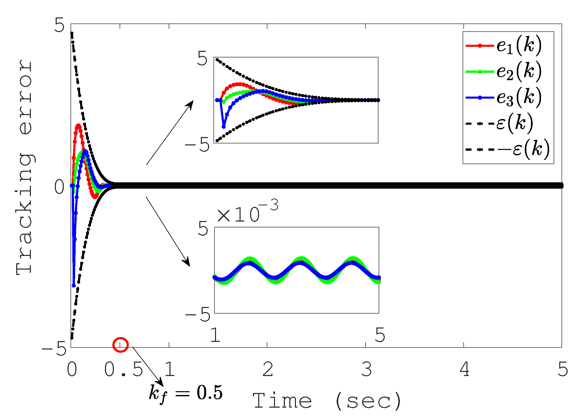
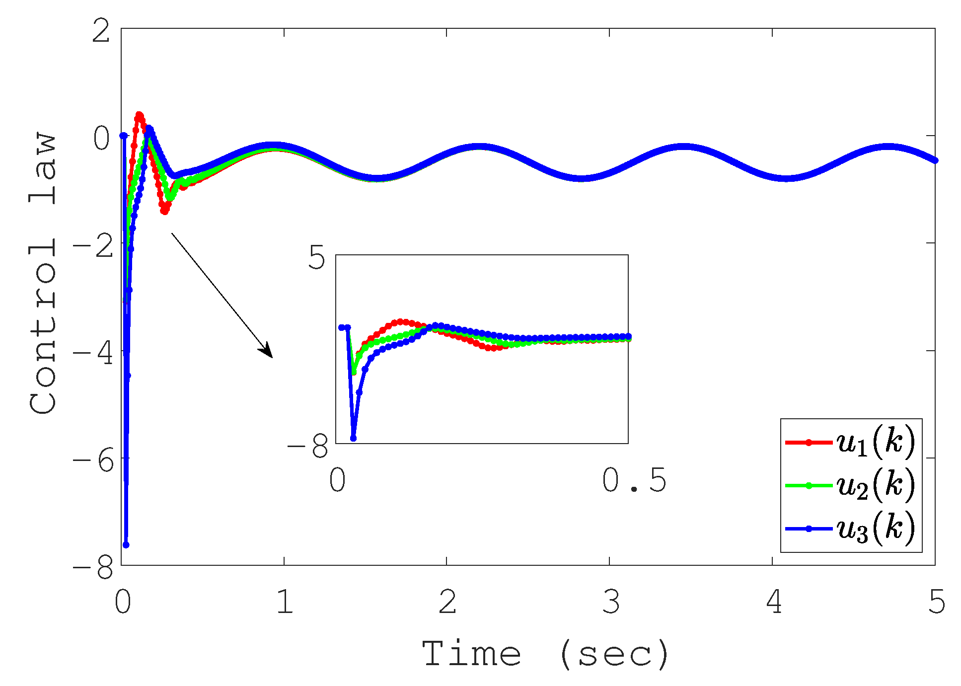
4.1. Tracking Results

The control results under the data-driven robust control strategy with performance constraints are shown in Figure 3, Figure 4, Figure 5, Figure 6 and Figure 7. The parameters are exhibited in

Table 1. Design parameters.

Control Unit	Design Parameters
Polynomial FTPF in (10)	${\epsilon }_0=5$, ${\epsilon }_{\infty }=0.05$, $k_f=0.5$;
Error transformation in (14)	${\phi }_h=0.8$, ${\phi }_l=0.8$;
Estimator for PJM in (22)	$\eta =0.1$, $\mu =10$;
DNDO in (30)	$K_1=0.95$, $K_2=0.2$, $\beta =0.3$, $\Omega =3$;
Control law in (39)	$\rho =0.5$, $\lambda =1$.

. The tracking diagram is exhibited in Figure 3, where the output $\mathit{y}(k)$ precisely tracks the output ${\mathit{y}}_d(k)$. The diagram of tracking error $\mathit{e}(k)$ is exhibited in Figure 4, and the error $\mathit{e}(k)$ draws into a prescribed region in a predetermined time. The diagram of estimator ${\widehat{\mathbf{\Gamma }}}_2(k)$ is exhibited in Figure 5, where ${\widehat{\mathbf{\Gamma }}}_2(k)$ draws into stable values. The diagram of the disturbance observation $\Delta \mathit{D}(k)$ is exhibited in Figure 6, and the disturbances are well observed. Additionally, the diagram of the control law $\mathit{u}(k)$ is exhibited in Figure 7, which means that the control scheme is feasible. From the control results of Figure 3, Figure 4, Figure 5, Figure 6 and Figure 7, all signals are bounded, and the control target in (7) is realized.

Meanwhile, Figure 8 shows a diagram of the error $\mathit{e}(k)$ under different predetermined times when $k_f=0.5$ s, $k_f=1$ s, $k_f=2$ s, and $k_f=5$ s. From Figure 7, the convergence time changes with the predetermined time $k_f$, and we can draw the following conclusions: (1) If $k_f$ decreases, the convergence time is shortened and system stability may be affected. (2) If $k_f$ increases, the convergence time is extended and steady accuracy may be affected. Therefore, ${\epsilon }_0$, ${\epsilon }_{\infty }$, and $k_f$ should be correctly chosen based on the system’s stability and steady accuracy, and different $k_f$ values can be chosen according to different tasks. Additionally, to effectively verify the theoretical claims about polynomial FTPFs through simulation results, based on the MATLAB(v2022) simulation tool, we compare the program running time using the polynomial FTPF and the exponential FTPF. The running time using the exponential function is $3.8$ s, while that using the polynomial FTPF is $3.5$ s, which means that the adoption of the polynomial FTPF can effectually reduce the running time, reflecting a decrease in the computational burden.

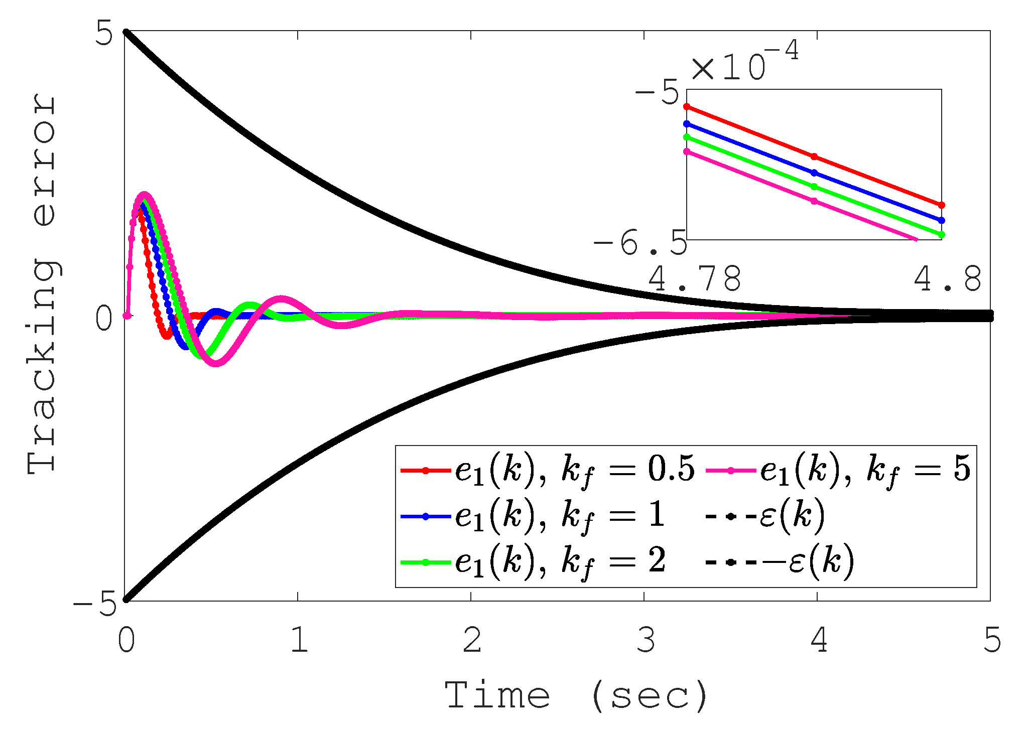
4.2. Comparative Simulations

To illustrate the advantages of the design control strategy, select the same parameters in

Table 2. Performance indexes under different control strategies in [11,16,37] and in this paper.

Performance Indexes	In [11]	In [16]	In [37]	In This Paper
Convergence time	1.3	1.2	1.1	0.5
Maximum overshoot	1.97	1.65	0.6	1.85
Steady error	−0.0557	−0.0447	−0.0533	−0.001

and compare the error $\mathit{e}(k)$ by using the control strategies in [11,16,37].

(i) The data-driven control strategy without performance constraints and without using DONO in [11] is considered as

$$\begin{array}{cc}\hfill \mathit{u}(k)=& \mathit{u}(k-1)+{\displaystyle \frac{\rho {\widehat{\mathbf{\Gamma }}}_2^T(k)\mathit{e}(k)}{\lambda +\parallel {\widehat{\mathbf{\Gamma }}}_2{(k)\parallel }^2}}+{\displaystyle \frac{\rho {\widehat{\mathbf{\Gamma }}}_2^T(k)\Delta {\mathit{y}}_d(k+1)}{\lambda +\parallel {\widehat{\mathbf{\Gamma }}}_2{(k)\parallel }^2}}-{\displaystyle \frac{\rho {\widehat{\mathbf{\Gamma }}}_2^T(k){\widehat{\mathbf{\Gamma }}}_1(k)\Delta \mathit{y}(k)}{\lambda +\parallel {\widehat{\mathbf{\Gamma }}}_2{(k)\parallel }^2}}.\hfill \end{array}$$

(54)

(ii) The data-driven robust control strategy without performance constraints in [16] is considered as

$$\begin{array}{cc}\hfill \mathit{u}(k)=& \mathit{u}(k-1)+{\displaystyle \frac{\rho {\widehat{\mathbf{\Gamma }}}_2^T(k)\mathit{e}(k)}{\lambda +\parallel {\widehat{\mathbf{\Gamma }}}_2{(k)\parallel }^2}}+{\displaystyle \frac{\rho {\widehat{\mathbf{\Gamma }}}_2^T(k)\Delta {\mathit{y}}_d(k+1)}{\lambda +\parallel {\widehat{\mathbf{\Gamma }}}_2{(k)\parallel }^2}}-{\displaystyle \frac{\rho {\widehat{\mathbf{\Gamma }}}_2^T(k){\widehat{\mathbf{\Gamma }}}_1(k)\Delta \mathit{y}(k)}{\lambda +\parallel {\widehat{\mathbf{\Gamma }}}_2{(k)\parallel }^2}}\hfill \\ \hfill & -{\displaystyle \frac{\rho {\widehat{\mathbf{\Gamma }}}_2^T(k)\Delta \widehat{\mathit{D}}(k)}{\lambda +\parallel {\widehat{\mathbf{\Gamma }}}_2{(k)\parallel }^2}}.\hfill \end{array}$$

(55)

(iii) The finite-time sliding-mode controller in [37] is considered as

$$\begin{array}{cc}\hfill \mathit{u}(k)=& -\tau \mathit{s}(k)-{\sigma \left|\mathit{s}(k)\right|}^r\mathrm{sign}(\mathit{s}(k)).\hfill \end{array}$$

(56)

where $\tau =10$, $\sigma =5$, and $r=0.9$ are bounded constants, and the sliding surface is set as

$$\begin{array}{cc}\hfill \mathit{s}(k)=& k_1{\mathit{e}}^{\mathbf{\Theta }}(k)+k_2{\left|{\mathit{e}}^{\mathbf{\Theta }}(k)\right|}^r\mathrm{sign}({\mathit{e}}^{\mathbf{\Theta }}(k))+{\mathit{e}}^{\mathit{\omega }}(k).\hfill \end{array}$$

(57)

where $k_1=0.5$ and $k_1=0.5$ are bounded constants, ${\mathit{e}}^{\mathbf{\Theta }}(k)={\mathbf{\Theta }}_d(k)-\mathbf{\Theta }(k)$, and ${\mathit{e}}^{\mathit{\omega }}(k)={\mathit{\omega }}_d(k)-\mathit{\omega }(k)$.

The diagram of the tracking error ${\mathit{e}}_1(k)$ under different control strategies in [11,16,37] and in this paper is displayed in Figure 9. Additionally, the performance indexes under different control strategies are shown in Table 2. Based on Figure 9 and Table 2, the control strategy in this paper yields several advantages. (1) Faster tracking speed: The error $\mathit{e}(k)$ shows a faster tracking speed compared to the control strategies in [11,16,37]. (2) Better tracking accuracy: The error $\mathit{e}(k)$ converges to a smaller boundary compared to the algorithm in [11,16,37]. (3) Convenient parameter design: The convergence boundary can be prescribed, allowing the control strategy to be designed according to different tasks. (4) No buffeting phenomenon: Compared with the finite-time control strategy in [37], the control strategy proposed does not have the buffeting phenomenon caused by the switching function.

5. Conclusions

The attitude tracking control issue for UUVs with disturbances is studied. Firstly, a new polynomial FTPF is introduced to reduce the computational burden, and the tracking error is converted into a constrained form using a transformation function. Then, an estimator is designed for estimating the PJM in a linearization model, and a DNDO is adopted for observing the unknown disturbances. With the help of the estimator for the PJM, the DNDO, and the constrained error, a data-driven robust attitude tracking control strategy with performance constraints is developed for UUVs. For our future research, filtering technology and a robust control method will be considered to deal with signal noise. Additionally, we will continue to conduct comparisons with other finite-time controllers to reinforce the innovation and competitive attributes of the proposed controller.

References

1. Kim, H.; Ahn, H.; Chung, Y.; You, K. Quadrotor position and attitude tracking using advanced second-order sliding mode control for disturbance. Mathematics 2023, 11, 4786. [Google Scholar] [CrossRef]
2. Chen, R.; Wang, Z.; Che, W. Adaptive sliding mode attitude-tracking control of spacecraft with prescribed time performance. Mathematics 2022, 23, 401. [Google Scholar] [CrossRef]
3. He, Y.; Wang, D.B.; Ali, Z.A. A review of different designs and control models of remotely operated underwater vehicle. Meas. Control. 2020, 53, 1561–1570. [Google Scholar] [CrossRef]
4. Cho, H.; Jeong, S.K.; Ji, D.H.; Tran, N.H.; Vu, M.T.; Choi, H.S. Study on control system of integrated unmanned surface vehicle and underwater vehicle. Sensors 2020, 20, 2633. [Google Scholar] [CrossRef] [PubMed]
5. Chen, J.; Han, Y.; Li, R.; Zhang, Y.; He, Z. Coupling dynamics study on multi-body separation process of underwater vehicles. Drones 2024, 8, 533. [Google Scholar] [CrossRef]
6. Johnson, M.A.; Moradi, M.H. PID Control; Springer-Verlag London Limited: London, UK, 2005; pp. 47–107. [Google Scholar]
7. Wang, L.; Zhang, W.; Zhang, Q.; Shi, H.; Zhang, R.; Gao, F. Terminal constrained robust hybrid iterative learning model predictive control for complex time-delayed batch processes. Nonlinear Anal. Hybrid Syst. 2023, 47, 101276. [Google Scholar] [CrossRef]
8. Wang, L.; Yu, J.; Li, P.; Li, H.; Zhang, R. A 2D-FM model-based robust iterative learning model predictive control for batch processes. ISA Trans. 2021, 110, 271–282. [Google Scholar] [CrossRef] [PubMed]
9. Wang, L.; Shen, Y.; Yu, J.; Li, P.; Zhang, R.; Gao, F. Robust iterative learning control for multi-phase batch processes: An average dwell-time method with 2D convergence indexes. Int. J. Syst. Sci. 2018, 49, 324–343. [Google Scholar] [CrossRef]
10. Bontempi, G.; Birattari, M.; Bersini, H. Lazy learning for local modelling and control design. Int. J. Control 1999, 72, 643–658. [Google Scholar] [CrossRef]
11. Hou, Z.; Jin, S. Model Free Adaptive Control: Theory and Applications; CRC Press: Boca Raton, FL, USA, 2013. [Google Scholar]
12. Xu, D.; Jiang, B.; Shi, P. A novel model-free adaptive control design for multivariable industrial processes. IEEE Trans. Ind. Electron. 2014, 61, 6391–6398. [Google Scholar] [CrossRef]
13. Hou, Z.; Xiong, S. On model-free adaptive control and its stability analysis. IEEE Trans. Autom. Control 2019, 64, 4555–4569. [Google Scholar] [CrossRef]
14. Yu, X.; Hou, Z.; Polycarpou, M.M. Distributed data-driven iterative learning consensus tracking for nonlinear discrete-time multiagent systems. IEEE Trans. Autom. Control 2021, 67, 3670–3677. [Google Scholar] [CrossRef]
15. Ma, Y.S.; Che, W.W.; Deng, C.; Wu, Z.G. Distributed model-free adaptive control for learning nonlinear MASs under DoS attacks. IEEE Trans. Neural Netw. Learn. Syst. 2021, 34, 1146–1155. [Google Scholar] [CrossRef] [PubMed]
16. Chen, R.Z.; Guo, X.G.; Li, Q.; Wang, J.L.; Guo, L. Disturbance-observer-based model-free adaptive active fault-tolerant consensus control for MASs with TVDAF. Automatica 2025, 173, 112114. [Google Scholar] [CrossRef]
17. Bechlioulis, C.P.; Rovithakis, G.A. Robust adaptive control of feedback linearizable MIMO nonlinear systems with prescribed performance. IEEE Trans. Autom. Control 2008, 53, 2090–2099. [Google Scholar] [CrossRef]
18. Bechlioulis, C.P.; Rovithakis, G.A. Prescribed performance adaptive control for multi-input multi-output affine in the control nonlinear systems. IEEE Trans. Autom. Control 2010, 55, 1220–1226. [Google Scholar] [CrossRef]
19. Bechlioulis, C.P.; Rovithakis, G.A. Robust partial-state feedback prescribed performance control of cascade systems with unknown nonlinearities. IEEE Trans. Autom. Control 2011, 56, 2224–2230. [Google Scholar] [CrossRef]
20. Zhang, J.X.; Yang, G.H. Prescribed performance fault-tolerant control of uncertain nonlinear systems with unknown control directions. IEEE Trans. Autom. Control 2017, 62, 6529–6535. [Google Scholar] [CrossRef]
21. Liu, D.; Yang, G.H. Data-driven adaptive sliding mode control of nonlinear discrete-time systems with prescribed performance. IEEE Trans. Syst. Man, Cybern. Syst. 2017, 49, 2598–2604. [Google Scholar] [CrossRef]
22. Huang, K.; Wang, H.; Pei, P.; Sun, H.; Shao, K. Preset trajectory based prescribed performance control for active anti-roll of automotives. Veh. Syst. Dyn. 2025, 1–22. [Google Scholar] [CrossRef]
23. Liu, Y.; Liu, X.; Jing, Y.; Zhang, Z. A novel finite-time adaptive fuzzy tracking control scheme for nonstrict feedback systems. IEEE Trans. Fuzzy Syst. 2018, 27, 646–658. [Google Scholar] [CrossRef]
24. Shao, K.; Zheng, J. Predefined-time sliding mode control with prescribed convergent region. IEEE/CAA J. Autom. Sin. 2022, 9, 934–936. [Google Scholar] [CrossRef]
25. Wang, H.; Bai, W.; Zhao, X.; Liu, P.X. Finite-time-prescribed performance-based adaptive fuzzy control for strict-feedback nonlinear systems with dynamic uncertainty and actuator faults. IEEE Trans. Cybern. 2021, 52, 6959–6971. [Google Scholar] [CrossRef] [PubMed]
26. Wang, X.; Niu, B.; Wang, H.; Zhao, X.; Chen, W. Prescribed performance-based finite-time consensus technology of nonlinear multiagent systems and application to FDPs. IEEE Trans. Circuits Syst. II Express Briefs 2022, 70, 591–595. [Google Scholar] [CrossRef]
27. Åström, K.J. Adaptive control. In Mathematical System Theory: The Influence of RE Kalman; Springer: Berlin/Heidelberg, Germany, 1995; pp. 437–450. [Google Scholar]
28. Feng, G. A survey on analysis and design of model-based fuzzy control systems. IEEE Trans. Fuzzy Syst. 2006, 14, 676–697. [Google Scholar] [CrossRef]
29. Liu, J.; Wang, X.; Liu, J.; Wang, X. Advanced Sliding Mode Control; Springer: Berlin/Heidelberg, Germany, 2011; pp. 81–96. [Google Scholar]
30. Han, J.Q. From PID to active disturbance rejection control. IEEE Trans. Ind. Electron. 2009, 56, 676–697. [Google Scholar] [CrossRef]
31. Zhao, Z.L.; Guo, B.Z. On active disturbance rejection control for nonlinear systems using time-varying gain. Eur. J. Control. 2015, 23, 62–70. [Google Scholar] [CrossRef]
32. Ran, M.; Li, J.; Xie, L. A new extended state observer for uncertain nonlinear systems. Automatica 2021, 131, 109772. [Google Scholar] [CrossRef]
33. Cao, P.; Gan, Y.; Dai, X. Finite-time disturbance observer for robotic manipulators. Sensors 2019, 131, 1943. [Google Scholar] [CrossRef]
34. Gu, S.; Zhang, J.; Liu, X. Finite-time variable-gain ADRC for master–slave teleoperated parallel manipulators. IEEE Trans. Ind. Electron. 2023, 71, 9234–9243. [Google Scholar] [CrossRef]
35. Cao, H.; Deng, Y.; Zuo, Y.; Li, H.; Wang, J.; Liu, X.; Lee, C.H. Improved ADRC with a cascade extended state observer based on quasi-generalized integrator for PMSM current disturbances attenuation. IEEE Trans. Transp. Electrif. 2023, 10, 2145–2157. [Google Scholar] [CrossRef]
36. Chi, R.H.; Yu, H.; Zhang, S.H.; Huang, B.; Hou, Z.S. Active disturbance rejection control for nonaffined globally Lipschitz nonlinear discrete-time systems. IEEE Trans. Autom. Control. 2023, 66, 5955–5967. [Google Scholar] [CrossRef]
37. Zhu, Z.; Xia, Y.; Fu, M. Attitude stabilization of rigid spacecraft with finite-time convergence. Int. J. Robust Nonlinear Control. 2011, 21, 686–702. [Google Scholar] [CrossRef]
Figure 1. Attitude tracking control framework.
Mathematics 13 01350 g001
Figure 2. System block diagram.
Mathematics 13 01350 g002
Figure 3. System output diagram.
Mathematics 13 01350 g003
Figure 4. Tracking error diagram.
Mathematics 13 01350 g004
Figure 5. Estimation diagram for PJM.
Mathematics 13 01350 g005
Figure 6. Disturbance observation diagram.
Mathematics 13 01350 g006
Figure 7. Control law diagram.
Mathematics 13 01350 g007
Figure 8. Tracking error diagram when k f = 0.5 s, k f = 1 s, k f = 2 s, and k f = 5 s.
Mathematics 13 01350 g008
Figure 9. Tracking error under different control strategies in [11,16,37] and in this paper.
Mathematics 13 01350 g009